Abstract
The prediction of casualties in earthquake disasters is a prerequisite for determining the quantity of emergency supplies needed and serves as the foundational work for the timely distribution of resources. In order to address challenges such as the large computational workload, tedious training process, and multiple influencing factors associated with predicting earthquake casualties, this study proposes a Support Vector Machine (SVM) model utilizing Principal Component Analysis (PCA) and Bayesian Optimization (BO). The original data are first subjected to dimensionality reduction using PCA, with principal components contributing cumulatively to over 80% selected as input variables for the SVM model, while earthquake casualties are designated as the output variable. Subsequently, the optimal hyperparameters for the SVM model are obtained using the Bayesian Optimization algorithm. This approach results in the development of an earthquake casualty prediction model based on PCA-BO-SVM. Experimental results indicate that compared to the GA-SVM model, the BO-SVM model, and the PCA-GA-SVM model, the PCA-BO-SVM model exhibits a reduction in average error rates by 12.86%, 9.01%, and 2%, respectively, along with improvements in average accuracy and operational efficiency by 10.1%, 7.05%, and 0.325% and 25.5%, 18.4%, and 19.2%, respectively. These findings demonstrate that the proposed PCA-BO-SVM model can effectively and scientifically predict earthquake casualties, showcasing strong generalization capabilities and high predictive accuracy.
1. Introduction
Earthquakes, as sudden natural disasters, have a profound impact on human society, resulting in casualties, structural damage, and economic losses. The accurate forecasting of earthquake casualties and resource requirements is crucial for effective rescue operations and post-disaster reconstruction efforts. Therefore, thoroughly considering the relationship between these two aspects and conducting scientific and rational predictions and planning can enable rescue organizations to more effectively strategize their relief efforts, optimize resource allocation, and enhance rescue efficiency, thereby minimizing the humanitarian disasters caused by catastrophic earthquakes [1,2,3,4]. Establishing a robust earthquake casualty prediction system and integrating scientific methodologies and statistical models holds significant importance for improving disaster response capabilities and mitigating disaster losses [5,6].
In general, there are two primary methods for predicting emergency material demand: direct and indirect approaches. Among the direct prediction methods identified in past research are the Relief Demand Forecast Model, the Fuzzy Clustering-based Model, the Bayesian Decision Framework, and the Fuzzy Rough Set Approach over Two Universes [7,8,9,10]. In order to make the model still have better expressiveness in different scenarios and in the absence of information, some new methods have emerged in recent years. Among them, Zheng et al. [11] proposed a co-evolutionary fuzzy deep transfer learning (CoFDTL) method for disaster relief demand prediction, which was applied to two real-world disaster events in China in 2018, which can be used to solve complex multi-task transfer learning problems with insufficient samples and uncertain information. Considering that it is challenging to collect and transmit the needs to remote shelters, a post-disaster demand forecasting system based on smartphone-based DTN using principal component regression analysis and case-based reasoning is proposed [12]. Rawls et al. [13] developed a heuristic called the Lagrangian L-shaped method (LLSM) to address large-scale instances of determining in advance the location and quantity of various types of emergency supplies to be deployed without being sure if or where a disaster occurred. Based on the background of public health emergencies, Ma et al. [14] established a metabolic gray model (1,1) (GM (1,1)) and a material demand prediction model to predict the number of infections and material demand and established a dual-objective optimization model to help improve the fairness of material distribution, but the prediction model is based on the first-order differential equation, assuming that the data change is exponential, and its applicability mainly lies in describing linear or near-linear changes, and it is difficult to capture complex nonlinear relationships. In the context of flood disaster, Chen et al. [15] used the improved ant colony optimization algorithm combined with the BP neural network to model the demand for emergency supplies, and the experimental results showed that the proposed algorithm IACO-BP is the most efficient and stable among the three algorithms, which can better assist the disaster situation. Al-Ghamdi et al. [16] proposed a PSO-ANN water demand forecasting model, which adjusted the hyperparameters of the artificial neural network by using PSO, and verified that the model is an accurate model for multivariate time series forecasting. Rostami-Tabar et al. [17] studied the effectiveness of parametric and non-parametric demand forecasting methods and found that the guided method has high performance in achieving higher service levels. Lin et al. [18] proposed a big data-driven dynamic estimation model of disaster relief material demand, which fuses Baidu big data and the dynamic population distribution of the multilayer perceptron (MLP) neural network to improve its accuracy and timeliness. In the earthquake scenario, Fei et al. [19] proposed a demand forecasting model for emergency supplies that combined the Dempster–Shafer theory (DST) and the case-based reasoning (CBR) method and established a dynamic demand forecasting model by using inventory management theory. Riachy et al. [20] proposed a framework for demand forecasting in the presence of a large number of data gaps and validated the proposed method on a real dataset of UK footwear retailers. Focusing on the seismic background, Dey et al. [21] used seismic data to analyze and predict intelligent solutions. In order to improve people’s ability to cope with earthquake disasters, Wei et al. [22] developed a semi-empirical model for casualty estimation. Horspool et al.’s [23] research focuses on understanding the background and causes of casualties caused by earthquakes.
Although the above methods have certain effectiveness in directly predicting the demand for emergency supplies, in the context of earthquakes, the method of indirectly predicting the demand for materials by predicting earthquake casualties has its unique advantages. Firstly, indirect forecasting can provide a more holistic view of the human impact of a disaster, allowing for a more accurate picture of changes in material needs. Direct forecasting methods tend to focus on a single demand estimate, while indirect forecasting combines multiple factors such as the number of casualties and the extent of damage to better adapt to complex disaster scenarios. Secondly, indirect forecasting methods are more flexible in the face of uncertainty. In particular, the suddenness and unpredictability of earthquakes make direct prediction more challenging, while indirect prediction can more effectively deal with the problem of information asymmetry by analyzing casualty data and historical cases, and then providing more reliable material demand estimates. In addition, the indirect prediction method can be derived from existing casualty prediction models in the absence of sufficient data, thereby reducing the dependence on a large amount of high-quality data. In summary, indirect forecasting has higher adaptability and flexibility than direct forecasting in emergency material needs assessment, which can provide strong support for decision-making in complex and uncertain environments, and lay the foundation for subsequent emergency material distribution and emergency response.
In order to scientifically and reasonably predict the demand for emergency supplies at each disaster site, experts and scholars from various countries have proposed a variety of prediction models for earthquake casualties in recent years, so as to indirectly predict the demand for emergency supplies. Based on the gray prediction model, Ma et al. [24] proposed a prediction method for the demand for emergency supplies based on the gray Markov model in order to improve the accuracy of forecasting the number of people affected by disasters and the demand for emergency materials, and the relative error of the proposed model was verified by comparing with the gray Markov model and the gray model. Chen et al. [25] proposed a gray prediction model with fewer parameters, which combined the three factors in the earthquake with the mortality rate to form the GM (0,3) model, which is a great improvement compared with the traditional model. However, the GM (0,3) model is more stringent in data conditions, especially for data with little or unstable historical data, and its prediction effect may be seriously affected. Wang et al. [26] constructed a multi-objective optimization model for the dispatch of emergency materials in multiple periods for uncertain sudden disasters and designed and improved the NSGA-II algorithm to solve the problem according to the characteristics of the proposed model, based on which the real data of the 2008 Wenchuan earthquake were combined with the simulation data and the corresponding examples, and, compared with the other three algorithms, the proposed model and algorithm were verified to effectively solve the problem of large-scale post-disaster emergency material distribution. Instead of making a reasonable prediction of the corresponding material demand, the method of combining simulated data with real data may lead to a certain deviation between the distribution and the actual demand. Hu et al. [27] constructed a prediction model for the demand for earthquake emergency supplies in the case of unclear information in the disaster area, used the PSO-BP hybrid neural network algorithm to predict the number of earthquake casualties, and combined the results with the inventory management knowledge to indirectly complete the prediction of the demand for materials in the disaster area. However, the BP neural network is sensitive to initial parameters, prone to overfitting, and prone to fall into local optimum, while SVM has advantages in dealing with multi-dimensional, small-sample, and nonlinear problems. By constructing a Genetic Algorithm based on Principal Component Analysis to improve the Support Vector Machine model to predict the number of earthquake casualties [28] and establish a robust wavelet v-SVM prediction model for the number of earthquake casualties, the model obtained has fast learning speed, strong stability and high prediction accuracy [29]. At the same time, compared with the swarm intelligence optimization algorithm, the Bayesian Optimization algorithm has significant advantages in dealing with high-dimensional and nonlinear problems, which can find the global optimal solution faster and with higher accuracy. In 2012, Snoek J et al. [30] first introduced a method of using the Bayesian Optimization algorithm to automatically adjust the hyperparameters in machine learning algorithms, which surpassed traditional manual tuning or brute force search methods and improved the performance of machine learning algorithms. Tang et al. [31] established a Bayesian network adaptability evaluation model and verified the applicability of the model in earthquake-prone counties in China.
The review of the aforementioned literature reveals that significant research outcomes have been achieved in casualty and emergency material demand forecasting across various contexts, which serve as references for this study. This work is based on the background of earthquake disasters. In past earthquake scenario studies, most scholars have utilized swarm intelligence optimization algorithms in combination with BP neural networks or Support Vector Machines (SVM) for casualty predictions. This study focuses on earthquake disasters and examines the prediction of casualties in past earthquake scenarios. Most researchers have employed swarm intelligence optimization algorithms in conjunction with BP neural networks or Support Vector Machines for casualty prediction. Existing methods include GA-SVM (Genetic Algorithm Support Vector Machine) and BO-SVM (Bayesian Optimization Support Vector Machine). Among these, GA-SVM has several disadvantages, including the risk of overfitting, high computational costs, and slow convergence rates. This model utilizes Genetic Algorithms for parameter optimization, which can lead to excessive complexity, particularly when training data are limited, thereby increasing the risk of overfitting. Additionally, the iterative process of the Genetic Algorithm requires substantial computation, resulting in prolonged training times, especially when dealing with large datasets. Due to the stochastic nature of Genetic Algorithms, the convergence of the model may necessitate a significant number of generations, which reduces efficiency.
Hence, based on previous studies, this paper proposes an earthquake casualty prediction model based on PCA-BO-SVM, and indirectly predicts the demand for emergency supplies based on the predicted number of casualties, which has the following advantages compared with the existing models:
- (1)
- The Principal Component Analysis method introduced by the model has the ability to reduce dimensionality, and PCA can reduce the dimension of input features, reduce the complexity of the model, reduce the risk of overfitting, and improve the computational efficiency, which makes the model more efficient when processing high-dimensional data. Through Principal Component Analysis, the model retains the most important information, avoids feature redundancy, and helps improve prediction accuracy.
- (2)
- Combined with Bayesian Optimization, the constructed PCA-BO-SVM model can be hyperparameter optimized in a lower dimension, reducing the probability of local optimum, and improving the global robustness of the model. The model can flexibly adapt to different feature combinations to improve the accuracy of earthquake casualty prediction.
- (3)
- The proposed model enhances the performance of the Support Vector Machine in earthquake casualty prediction by combining PCA dimensionality reduction technology and Bayesian Optimization hyperparameter selection. PCA plays an important role in reducing dimensions, improving computational efficiency, and improving model interpretability, while Bayesian Optimization ensures the optimization of hyperparameter selection, thereby improving the accuracy and credibility of the prediction results, effectively overcoming the computational complexity and local optimal problems existing in GA-SVM and BO-SVM, and providing a more reliable and efficient solution for earthquake casualty prediction.
The organization of this study is structured as follows: Section 2 presents the key steps and processes involved in the overall research. Section 3 describes the principles used to construct the PCA-BO-SVM model. Section 4 is dedicated to the experimental part, where the developed model is utilized for casualty prediction and result analysis. Section 5 focuses on estimating the demand for emergency materials. Finally, Section 6 provides the conclusions and future outlook of this study.
2. Research Design
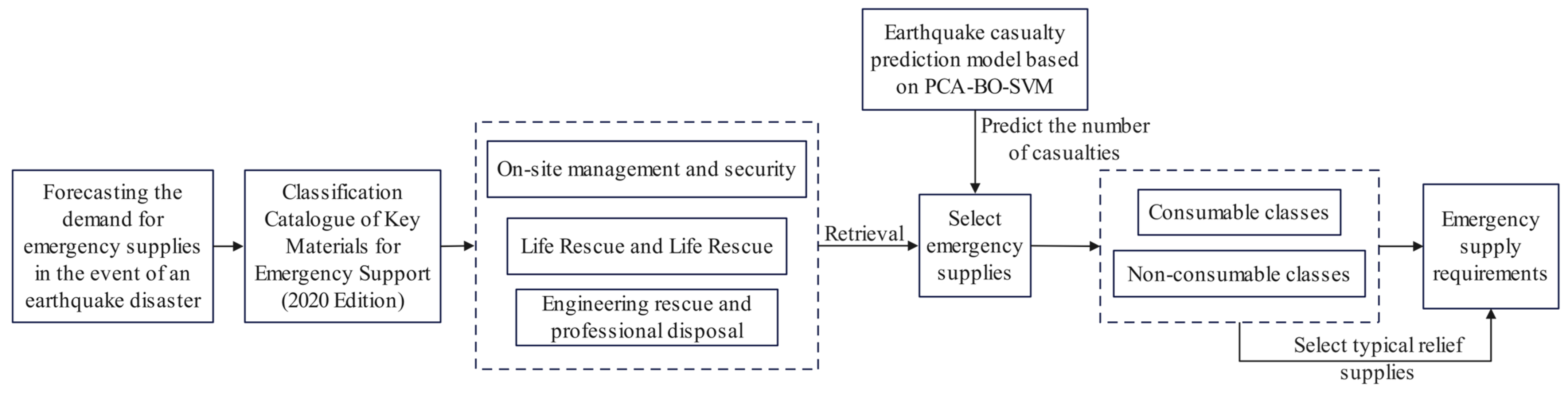
Figure 1 shows the overall flow chart of the post-earthquake casualty and emergency material demand forecast based on PCA-BO-SVM. The key steps are as follows:
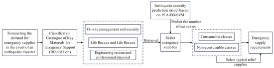
Figure 1.
Process of forecasting the demand for emergency supplies during earthquake disasters.
- Step 1: Identify the types of emergency resources to be predicted in the aftermath of an earthquake. To alleviate the survival pressures faced by affected populations and to ensure their basic living needs are met, this study references the “Catalogue of Key Emergency Support Materials (2020)” and selects resources categorized under life rescue and livelihood assistance as the focus of the research.
- Step 2: Develop the earthquake casualty prediction model based on PCA-BO-SVM. By utilizing historical data from 171 destructive earthquakes in China between 1966 and 2023, Principal Component Analysis is employed to reduce the dimensionality of the original data. Subsequently, the Bayesian Optimization algorithm is used to identify the optimal hyperparameters for the Support Vector Machine, thereby establishing the PCA-BO-SVM-based earthquake casualty prediction model.
- Step 3: Determine the typical emergency resources required and their respective demand quantities. Considering the most urgent needs of disaster victims, the resources are categorized into consumable and non-consumable types. Consumable resources include drinking water, compressed biscuits, and medical supply kits, while non-consumable resources consist of tents and clothing. Finally, based on the developed model, this study predicts the number of casualties resulting from an earthquake and estimates the demand for typical emergency resources.
3. Fundamental Principles
3.1. Principal Component Analysis
Principal Component Analysis (PCA) is a widely used multivariate statistical analysis method and a linear algebra technique based on eigenvalue decomposition. Its primary objective is to transform the original variables into a set of independent principal components through linear transformations, thereby reducing the dimensionality of the data while retaining critical information. This is achieved by preserving the first few principal components, which capture the essence of the data. PCA aids in identifying patterns and structures within the data, enhancing interpretability and explainability, making it a common technique in data analysis and data mining. The core concept of PCA is to identify the direction of maximum variance among the data variables and to project the original data in these directions, allowing the new principal components to explain the variability of the original data to the greatest extent. This process facilitates a better understanding and interpretation of the patterns and relationships present in the data. PCA determines the weight coefficients of the principal components by calculating eigenvalues and eigenvectors, thus achieving the goals of dimensionality reduction and feature extraction. The specific methodology is as follows:
- (1)
- Assume that X consists of m samples , with each sample being n-dimensional, which corresponds to the following matrix:In Equation (1), denotes the n feature for the m sample.
- (2)
- Feature Parameter Standardization: To eliminate the dimensional and variance differences among different feature parameters and ensure a relatively fair influence of each feature parameter on the results of Principal Component Analysis, standardization is employed. This process enables the data distribution of each feature parameter to have similar scales and variances, thus preventing any feature parameter with a large numerical range or high variance from disproportionately affecting the computation of principal components. Consequently, this approach guarantees the accuracy and reliability of the principal components. The standardized data are more conducive to performing Principal Component Analysis, resulting in outcomes that are more interpretable and stable.
In Equation (4), represents the standardized feature indicator; denotes the mean of feature indicator j; indicates the variance of feature indicator j.
- (3)
- Calculate the correlation coefficient matrix :
According to Equation (5), the correlation coefficient matrix can be calculated as follows:
In Equation (6), represents the correlation coefficients of the standardized feature indicators, and .
- (4)
- Calculate the eigenvalues and contribution rates to determine the principal components.
The eigenvalues of the correlation coefficient matrix are computed, with their corresponding eigenvectors denoted as , where , resulting in n new indicator variables formed from the eigenvectors:
In Equation (7), refers to the n principal component, and the contribution rate and cumulative contribution rate of the eigenvalue can be calculated as described in Equations (8) and (9):
In summary, Principal Component Analysis (PCA) is a statistical technique employed for dimensionality reduction. It achieves this by projecting the original data into a new coordinate system through linear transformations, where the first principal component accounts for the maximum variance, followed by subsequent components in decreasing order of variance.
The integration of PCA into Support Vector Machines (SVM) enhances performance for several compelling reasons:
- (1)
- Dimensionality Reduction and Information Retention: PCA effectively compresses redundant features within high-dimensional datasets, thereby reducing dimensionality while preserving the most critical information. This process not only alleviates computational burdens but also lowers model complexity, consequently reducing the risk of overfitting.
- (2)
- Improved Computational Efficiency: The training process of SVM can become exceedingly time-consuming and complex in high-dimensional spaces. By employing PCA for dimensionality reduction, the number of features input into the SVM is significantly decreased, resulting in reduced training times and enhanced computational efficiency.
- (3)
- Enhanced Model Interpretability: Following dimensionality reduction, the principal components provided by PCA often offer clearer insights into the underlying data structure. This clarity aids researchers in better understanding the key factors influencing earthquake casualties, thereby supporting informed decision-making.
Overall, the application of PCA not only optimizes the performance of SVM but also contributes to a more efficient and interpretable modeling process in the context of earthquake casualty prediction.
3.2. Bayesian Optimization Algorithm
Bayesian Optimization (BO) is a powerful method for optimizing black-box functions, based on Bayes’ theorem and Gaussian processes. It demonstrates significant advantages when addressing high-dimensional and nonlinear problems. Compared to other algorithms, Bayesian Optimization seeks the global optimum by constructing a probabilistic model that represents the objective function, with the goal of minimizing or maximizing an unknown objective function. The core of Bayesian Optimization lies in establishing a probabilistic model that represents the objective function and iteratively updating this model to identify the global optimum. In each iteration, the algorithm selects a sample point for evaluation and, based on the results, updates the probabilistic model. This process is repeated until a predefined termination condition is met.
The Bayesian Optimization algorithm exhibits high sampling efficiency and robustness, making it widely applicable in various fields, including hyperparameter optimization, automated parameter tuning, and the training of machine learning models. For hyperparameter optimization using Bayesian methods, the optimizer iteratively conducts a limited number of experiments within the hyperparameter search space to optimize f and obtain the optimal combination of hyperparameters:
Bayesian Optimization employs the principles of Bayesian statistics to guide the process of hyperparameter selection by constructing a probabilistic model of the objective function, typically represented as a Gaussian process. This process encompasses several key steps:
- (1)
- Building the Surrogate Model: In the initial phase, Bayesian Optimization randomly selects several hyperparameter combinations and evaluates the corresponding model performance metrics (e.g., prediction accuracy). The results of these evaluations are then utilized to construct a surrogate model that approximates the objective function within the hyperparameter space.
- (2)
- Utilization of Acquisition Functions: Based on the existing data, Bayesian Optimization employs acquisition functions (such as expected improvement or upper confidence bound) to determine the next hyperparameter combination to evaluate. These acquisition functions facilitate a balance between exploration (testing new hyperparameter combinations) and exploitation (optimizing known high-performing hyperparameter combinations).
- (3)
- Iterative Optimization: Through the continuous iteration of these steps, Bayesian Optimization progressively narrows the hyperparameter search space and ultimately identifies the optimal hyperparameter combination.
The choice of hyperparameters has profound implications for model performance, primarily reflected in several aspects:
- (1)
- Model Complexity: Hyperparameters, such as the regularization parameter C in SVM, play a crucial role in adjusting model complexity. The selection of C influences the model’s susceptibility to overfitting or underfitting. A high C value may lead to exceptional fit on training data but result in poor generalization to testing data, thereby increasing the risk of overfitting. Conversely, a low C value may prevent the model from capturing complex patterns in the data, manifesting as underfitting. Thus, careful selection of C is essential, and Bayesian Optimization provides a precise mechanism for tuning this parameter.
- (2)
- Kernel Function Selection and Parameters: In SVM, the choice of the kernel function and its parameters (e.g., σ in Gaussian kernels) significantly affect model performance. Different kernel functions and their associated parameters determine the flexibility of the decision boundary. Selecting inappropriate kernel parameters may result in a loss of accuracy when modeling complex data structures. Bayesian Optimization can effectively explore kernel parameters, facilitating the model’s adaptation to underlying data patterns.
- (3)
- Model Generalization Capability: The selection of hyperparameters directly influences the model’s ability to generalize, which refers to its performance on unseen data. Fine-tuning hyperparameters through Bayesian Optimization can enhance the model’s adaptability to new data, thereby reducing its susceptibility to overfitting on a specific training set and improving predictive accuracy.
In the context of earthquake casualty prediction, Bayesian Optimization serves as an efficient method for hyperparameter selection, significantly enhancing the performance of models such as Support Vector Machines (SVM). The selection of hyperparameters, which are predetermined prior to model training, is critical for the overall effectiveness of the model.
3.3. Support Vector Machine
Support Vector Machine (SVM) is a supervised learning algorithm based on statistical learning theory, which demonstrates significant advantages in handling nonlinear, small-sample, and high-dimensional data [8]. The core idea is to transform the input vectors of the training sample set through a nonlinear mapping into feature vectors in a high-dimensional space, thereby converting the nonlinear classification problem into a linear one in that space. By applying the nonlinear mapping , the input data is projected into a high-dimensional space, which can be expressed mathematically as follows: . By optimizing to solve for the weight vector and threshold, the Support Vector Machine obtains the optimal decision hyperplane, allowing for effective classification of the samples. The weight vector and the threshold can be derived from the following function to obtain the optimal solution:
In Equation (11), represents the penalty parameter, which plays a crucial role as an important tuning parameter in the Support Vector Machine model. It controls the complexity of the model, prevents overfitting, regulates the margin size, and addresses class imbalance. By constructing the Lagrangian function, the complex quadratic programming problem described above can be transformed into its dual problem. The solutions are obtained by solving for the original variables and the Lagrange multipliers, utilizing the Karush–Kuhn–Tucker (KKT) conditions to achieve the optimal solution. This transformation simplifies the solving process and enhances computational efficiency. The dual problem can be expressed as follows:
In Equation (13), the kernel function of the Support Vector Machine is denoted as , while and represent the Lagrange multipliers. The optimal solution can be obtained as follows:
The radial basis function (RBF) kernel of the SVM can be expressed as follows:
After calculations, the final regression function of the SVM is given by the following:
In Equation (16), and represent the kernel function; and denote the Laplace operators; and the bias term is represented by .
4. Earthquake Casualty Prediction Model
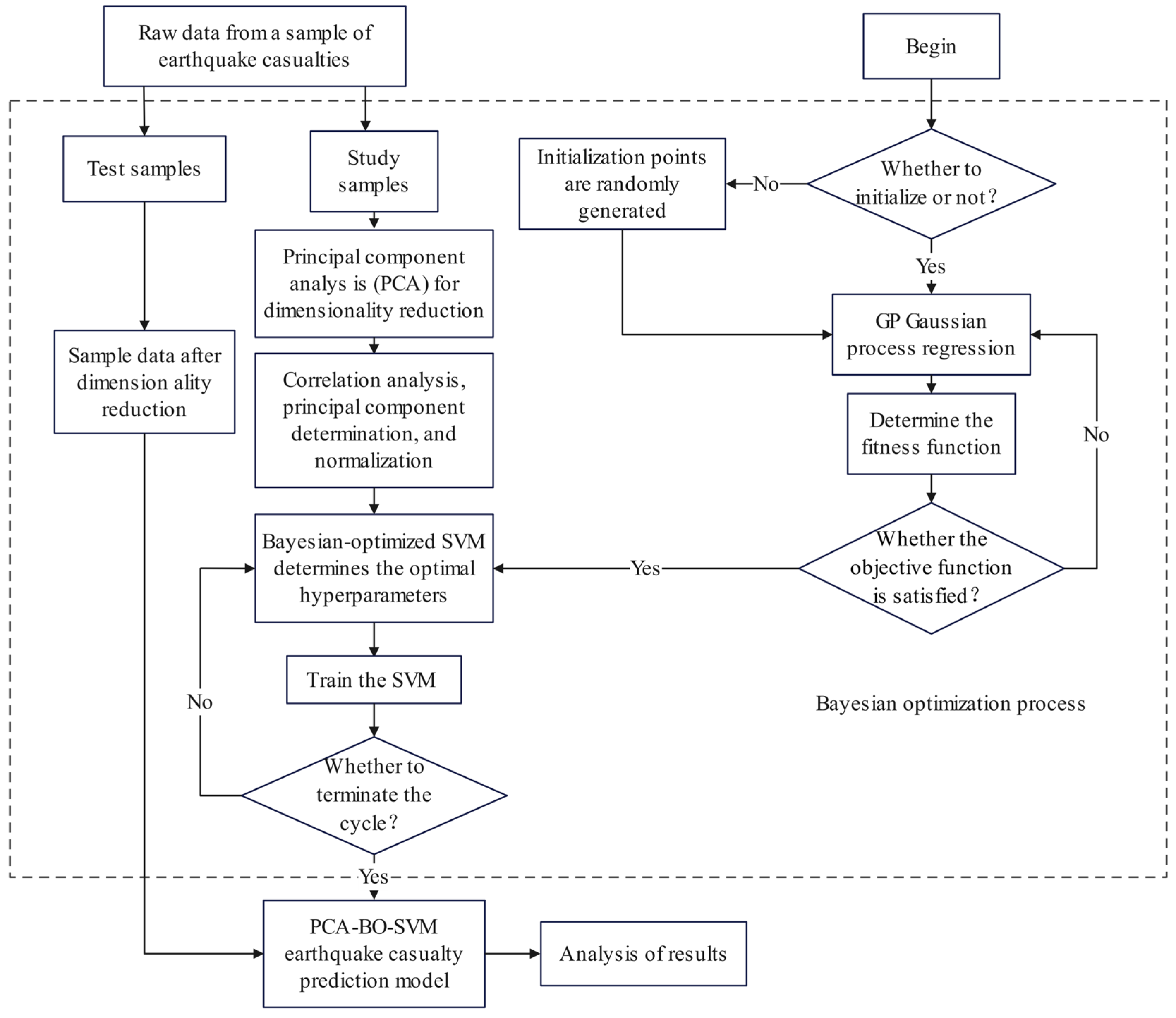
Figure 2 illustrates the modeling process for predicting earthquake casualties based on PCA-BO-SVM. The relevant steps are as follows:
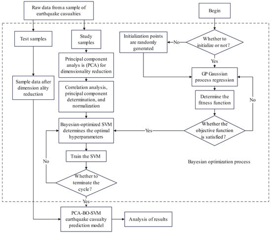
Figure 2.
PCA-BO-SVM flow chart.
- Step 1: Utilize Principal Component Analysis (PCA) to perform dimensionality reduction, correlation analysis, and normalization on the collected raw data, and to determine the principal components.
- Step 2: Select the fitness function. The quality of the parameters is assessed using the Mean Absolute Percentage Error (MAPE) as the criterion for the selection of the fitness function.
- Step 3: Employ the Bayesian Optimization (BO) algorithm to optimize the hyperparameters of the SVM. Set up the Bayesian optimizer to search for the optimal SVM hyperparameters, and optimize the BO-SVM model using the normalized training samples.
- Step 4: Output the best hyperparameters, train the SVM model, and construct the PCA-BO-SVM prediction model for earthquake casualties. Subsequently, perform predictions on the test samples and analyze the results.
- Step 5: Analyze and compare the running efficiency and prediction accuracy of different models to draw conclusions.
4.1. Data Preparation
In this paper, 171 destructive earthquakes of magnitude 5 or higher that occurred in China from 1966 to 2023 were selected as sample data; the first 163 earthquakes were used as learning samples and the last 8 earthquakes were used as test samples. These data come from the “China Earthquake Cases” published by the Seismological Press and the following websites: the National Seismological Data Center of China (https://data.earthquake.cn), the China Earthquake Network (https://news.ceic.ac.cn), the Ministry of Emergency Management of the People’s Republic of China (https://www.mem.gov.cn), and the Chinese Statistical Database (https://www.hongheiku.com). Detailed information is provided in Table 1. Based on the analysis of factors influencing earthquake casualty predictions discussed in [25], this study focuses on seven influencing factors for destructive earthquake disasters: time, earthquake intensity, occurrence time, magnitude, population density in the disaster area, seismic resistance level of buildings, and earthquake forecasting capability. For the time variable, values 1 and 2 represent night and day, respectively, where night refers to earthquakes occurring between 19:00 and 6:00, during which escape is hindered, while day refers to earthquakes occurring between 6:00 and 19:00. Earthquake intensity is expressed using Roman numerals IV to XI, with larger numbers indicating greater intensity and destructiveness in the affected areas; the minimum earthquake intensity in the selected samples is IV (4). Regarding magnitude, larger numbers correspond to higher magnitudes; this study considers earthquakes with magnitudes ranging from 4.0 to 8.1 that caused destruction. The population density in the disaster area refers to the ratio of the number of people affected in the area after a natural disaster, expressed in “people/area”. Population density is an important indicator that reflects the degree of population concentration and density in the disaster area. In similar circumstances, high population density often implies a greater number of people affected, which is significant for disaster management and rescue efforts. For seismic resistance levels, higher numbers indicate greater seismic resistance of buildings. In this study, building seismic resistance is categorized into nine levels, represented by the numbers 1 to 9. The forecasting capability is indicated by values 0, 1, and 2, where 0 denotes no warning, 1 indicates a warning but with low accuracy, and 2 represents a warning with high accuracy.

Table 1.
Raw data.
4.2. Principal Component Analysis
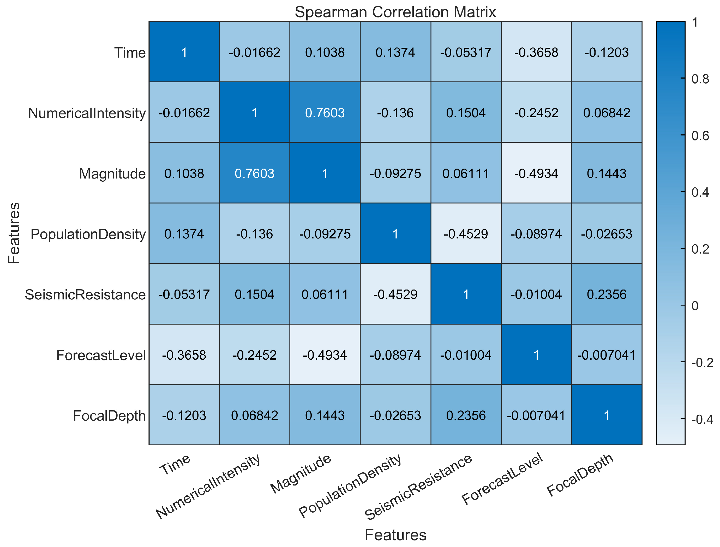
This study employed Principal Component Analysis (PCA) to conduct a correlation analysis and dimensionality reduction on seven influencing factors: time, earthquake intensity, occurrence time, magnitude, population density in disaster areas, seismic resistance of buildings, earthquake prediction capability, and focal depth. The results of this processing are illustrated in Figure 3, where the correlation coefficient heatmap uses color intensity to represent the magnitude of the correlation coefficients. Darker colors indicate stronger correlations, while lighter colors indicate weaker correlations. This visualization allows for an intuitive assessment of which variables exhibit strong correlations, thereby facilitating further analysis of the relationships and influences between the variables.
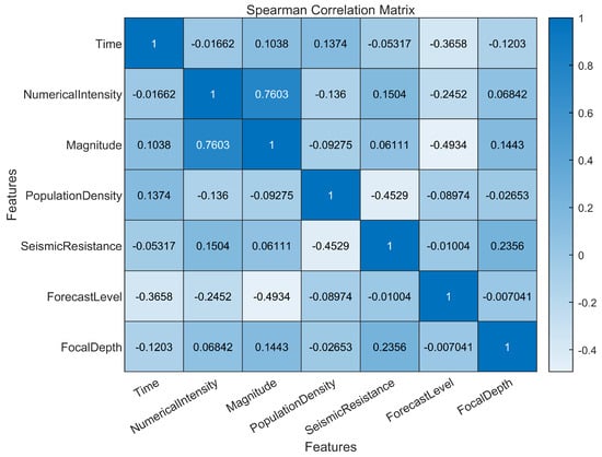
Figure 3.
Correlation coefficient heatmap.
Figure 3 shows the correlation between the features, and it can be seen that there is a significant positive correlation between seismic intensity and magnitude. There is a significant negative correlation between the seismic level of buildings and population density, the predicted level, and the earthquake magnitude. In the context of earthquake casualty prediction, the correlation of various features reveals the impact on casualty prediction and provides a data basis for follow-up research. Figure 3 can quickly identify which features have high correlation and which features have weak relationships with each other, and strong correlation features may bring better prediction performance in model training, which is crucial for subsequent model training and prediction results.
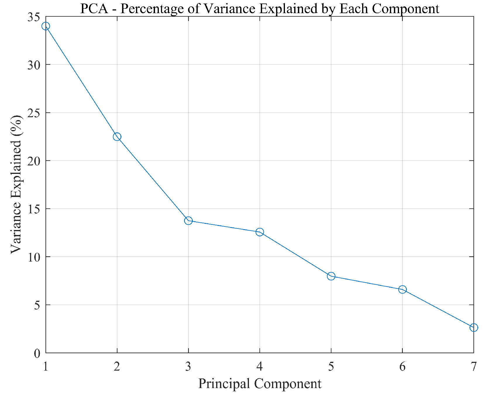
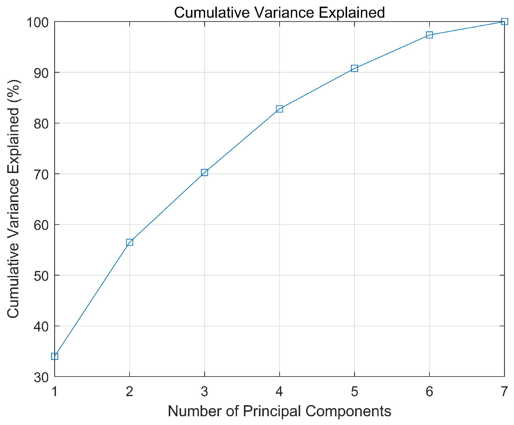
The contribution rates of each principal component, normalized eigenvalues, and cumulative contribution rates are presented in Table 2, with the contribution rates and cumulative contribution rates depicted in Figure 4 and Figure 5, respectively.
Table 2.
Normalized eigenvalues, contribution rates, and cumulative contribution rates.
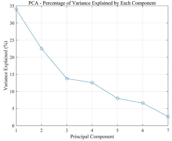
Figure 4.
Contribution rate of each component.
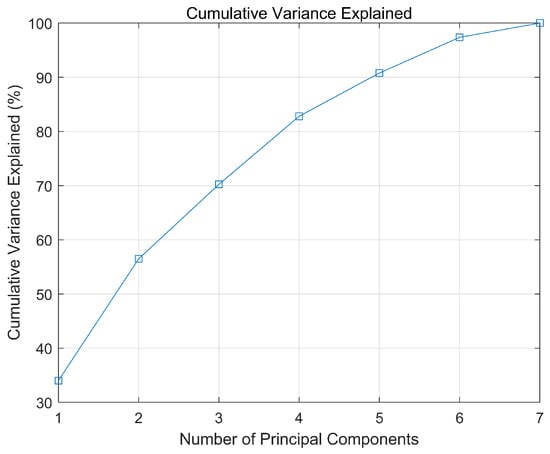
Figure 5.
Cumulative contribution rate.
To capture the majority of the information contained in the original data, it is common practice to select principal components with a cumulative contribution rate of over 80%. Therefore, based on Table 2, the first four principal components were chosen, resulting in a dimensionality reduction from seven-dimensional data to four-dimensional data. Using to represent the seven original variables, the expressions for the four principal components are provided in Equation (17). The four principal components were then normalized using Equation (18), which served as the input variables for constructing the SVM model. This approach not only reduces computational complexity and enhances the model’s generalization ability to avoid overfitting but also improves operational efficiency. The normalization results are presented in Table 3.
Table 3.
Principal component normalization data.
In Equation (17), represents time, indicates earthquake intensity, denotes magnitude, signifies population density, represents seismic resistance, indicates prediction capability, and denotes focal depth.
In Equation (18), the denominator represents the maximum value of each principal component, while denotes the minimum value of each principal component. The numerator corresponds to the value of the i sample for each principal component, and the normalized value for each principal component is represented by .
4.3. Model Building
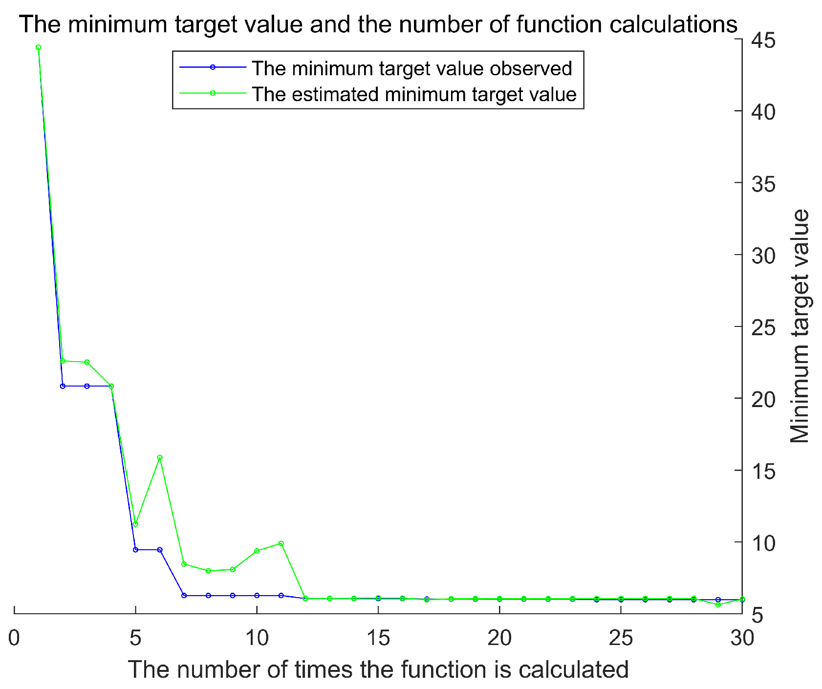
To obtain the optimal hyperparameters for the Support Vector Machine (SVM), this study implemented a program based on the Bayesian Optimization Support Vector Machine using MATLAB R2020b. The number of earthquake casualties was designated as the output variable, while the four principal components listed in Table 3 served as the input variables. After extensive training, the optimal fitness curve was achieved, as illustrated in Figure 6. The minimum objective value and the number of function evaluations are shown in Figure 7. Additionally, the Bayesian Optimization process took 17.42 s to identify the best hyperparameters, demonstrating a high level of operational efficiency.
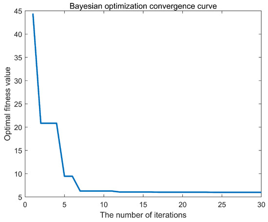
Figure 6.
Bayesian Optimization.
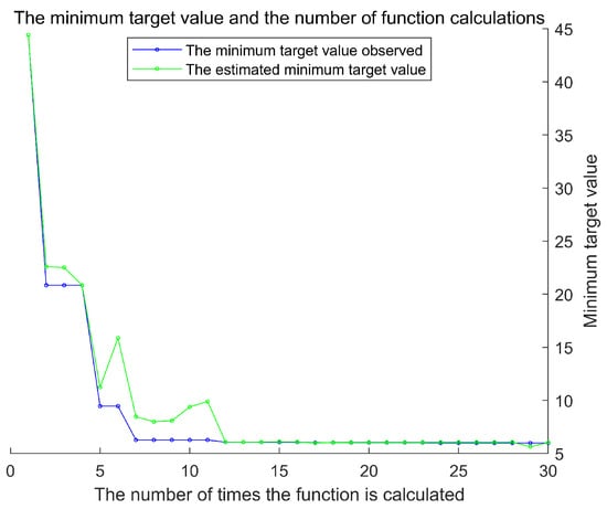
Figure 7.
The minimum target value and the number of function calculations.
4.4. Prediction Results and Analysis
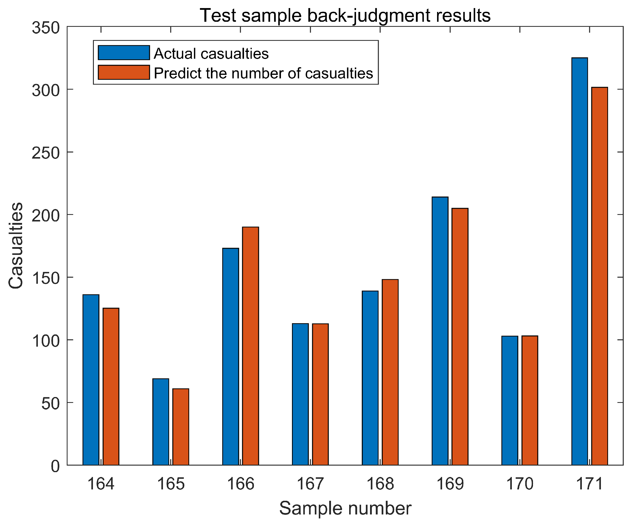
Using the constructed PCA-BO-SVM model, we performed predictions and validations on the test samples, and the results are presented in Figure 8. As shown in the results depicted in Figure 8, by comparing with historical data, it can be seen that there is not much difference between the predicted casualty and the actual casualty number, indicating that the PCA-BO-SVM model can effectively capture the key factors that affect the casualty number when processing the data. The average accuracy of the prediction results is 94.25%, which shows the accuracy of the prediction of the proposed model, and it can be seen that the prediction model based on Principal Component Analysis and Bayesian Optimization Support Vector Machine (PCA-BO-SVM) has a high consistency with the actual value.

Figure 8.
Results of test sample reassessment.
To further evaluate the predictive performance of the models, we employed the Genetic Algorithm Optimized Support Vector Machine (GA-SVM) model, the Bayesian Optimized Support Vector Machine (BO-SVM) model, and the Principal Component Analysis and Genetic Algorithm Optimized Support Vector Machine (PCA-GA-SVM) model to make predictions using the test samples provided in this study. This analysis allows for a comparison of the predictive performance across the different models. The prediction results for the four models are presented in Table 4, which includes the runtime for each model, predicted values, accuracy, relative error, maximum error, minimum error, average error, and average accuracy.
Table 4.
Casualty prediction results from different models.
As shown in Table 4, the PCA-BO-SVM model constructed in this study has a runtime of 17.42 s, making it the fastest among the models evaluated, while also achieving the highest accuracy and the lowest average error. Compared to the GA-SVM, BO-SVM, and PCA-GA-SVM models, the PCA-BO-SVM model exhibits a reduction in average error of 12.86%, 9.01%, and 2%, respectively, while improving average accuracy and operational efficiency by 10.1%, 7.05%, and 0.325% and 25.5%, 18.4%, and 19.2%, respectively. These results indicate that the PCA-BO-SVM model possesses high operational efficiency, average accuracy, and strong generalization capability, providing a scientifically sound basis for predicting casualties from earthquake disasters and establishing a foundation for demand forecasting.
The relative errors of the prediction results from the four models are illustrated in Figure 9. According to the relative errors of the predictions from various models presented in Figure 9, the PCA-BO-SVM model demonstrates the best performance. Without conducting Principal Component Analysis, both the GA-SVM and BO-SVM models exhibit relatively large errors, while the results of the BO-SVM model outperform those of the GA-SVM model. This indicates that the Bayesian Optimization Support Vector Machine (BO-SVM) is more effective than the Genetic Algorithm (GA) in this context. It is evident that the BO-SVM has superior convergence and robustness when handling high-dimensional data and complex optimization problems, allowing it to find the global optimum more rapidly. Moreover, it performs exceptionally well in managing noisy data and non-convex optimization issues, making it well suited for practical applications. Figure 9 illustrates the significant improvement in performance resulting from dimensionality reduction through principal component analysis, leading to better data analysis.
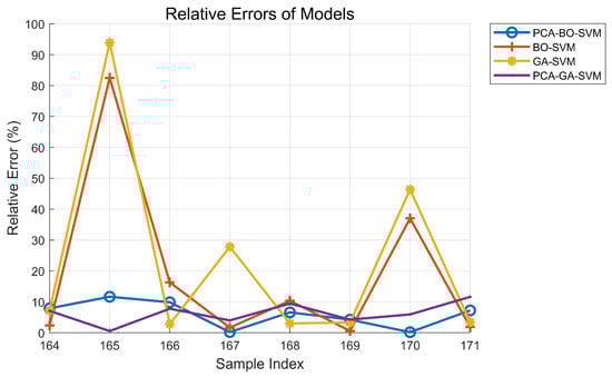
Figure 9.
Relative errors of prediction results from four models.
4.5. Discussion
In general, the PCA-BO-SVM model shows higher prediction accuracy and operational efficiency in earthquake casualty prediction, and the implementation of the model can effectively improve the foresight of disaster management, marking the importance of data-driven decision-making in the field of public safety and disaster management, and also providing a certain scientific basis for government decision-makers in emergency response, material allocation, and post-disaster recovery. However, disaster preparedness depends not only on understanding natural phenomena and data collection, but also on a comprehensive assessment of social risks. The applicability of the model has yet to be verified, and its accuracy and effectiveness are limited by data quality and model complexity. At the same time, the prediction of emergency supplies should also consider the influence of other factors in future research, so as to enrich the types of emergency supplies and items to meet the needs of disaster victims more scientifically and reasonably.
In this paper, the framework and methodology of the proposed model may also have the potential to adapt to other types of natural disasters, such as floods, typhoons, or fires. However, the specific verification also needs to be carried out through the corresponding PCA processing and Bayesian Optimization of the characteristic data of different disaster types, and the model is redesigned to predict the number of casualties or other impact indicators under different scenarios. The accuracy of prediction accuracy of the model is not only achieved through PCA dimensionality reduction and Bayesian Optimization but also depends on the quality of the data, which brings challenges to different research backgrounds and adaptation ranges. In order to solve this problem, in the future, we can explore the hybrid model method, consider more input features into the model, and use improved algorithms to integrate the model to enhance the robustness and generalization ability of the model. We can overcome bottlenecks through method innovation, data integration, and interdisciplinary collaboration, and further improve the accuracy and adaptability of the model so that it can more comprehensively handle various nonlinear relationships and adapt to different disaster scenarios.
5. Analysis of Emergency Material Demand for Earthquakes
In the initial phases of an earthquake disaster, the most pressing needs of affected populations primarily include consumable supplies such as drinking water, compressed biscuits, and bread. Non-consumable supplies are predominantly focused on items for warmth, such as tents and clothing. Additionally, medical supply kits are essential. This study selects drinking water, compressed biscuits, medical supply kits, tents, and clothing as representative emergency supplies from the aforementioned categories.
When calculating the demand for these typical emergency supplies, this study incorporates regional coefficients and seasonal coefficients [32], drawing on insights from the existing literature and research. The calculation formula is as follows:
In Equation (19), represents the total demand for supplies, indicates the per capita demand for the k type of supply, R denotes the predicted number of casualties in the earthquake-affected area, signifies the seasonal variation coefficient, represents the regional variation coefficient, and indicates the number of days for which emergency supplies are needed. The following table (Table 5) presents typical standards for per capita demand for emergency supplies, including a medical supply pack that contains anti-inflammatory medications, iodine tincture, glucose, gauze, and other items.
Table 5.
Typical per capita demand for emergency supplies.
Estimation of Emergency Supply Demand
Using the PCA-BO-SVM model developed in this study to predict the number of casualties due to earthquakes, we conducted a demand forecast for emergency supplies, taking the prediction result for 3.4 (as shown in Table 6) as an example. In the demand forecasting formula (Equation (19)), we set the regional variation coefficient to 0.9, the seasonal variation coefficient for consumable materials to 1.2, and the seasonal variation coefficient for non-consumable materials to 1.5, with the required supply of emergency materials set to 15 days. The results for the required quantities of emergency supplies are presented in Table 7.
Table 6.
Comparison of actual and predicted casualties in the disaster-affected area.
Table 7.
Predicted demand for supplies at various disaster sites.
6. Conclusions
In the aftermath of an earthquake, it is crucial to scientifically and rationally predict the number of casualties to effectively implement emergency rescue measures and estimate the demand for emergency supplies. This predictive capability facilitates a more efficient response to earthquake disasters and is vital for guiding the allocation of relief resources. Moreover, it plays a key role in minimizing both human casualties and property losses. Therefore, this study investigates the prediction of casualties resulting from seismic events and the demand for emergency resources, leading to the following conclusions:
- (1)
- Principal Component Analysis (PCA) was employed to reduce the dimensionality of the raw data from 171 destructive earthquakes in China, which included seven influential factors: time, earthquake intensity, occurrence timing, magnitude, population density in disaster areas, building seismic resistance, and earthquake forecasting capability. This dimensionality reduction from seven to four dimensions significantly enhanced operational efficiency and reduced model complexity.
- (2)
- The Bayesian Optimization (BO) algorithm exhibits superior convergence and robustness when dealing with high-dimensional data and complex optimization problems. It can more rapidly locate the global optimum and demonstrates exceptional performance in handling noisy data and non-convex optimization issues, making it more adaptable to real-world applications. Through Bayesian Optimization, this study configured the optimizer to search for optimal SVM hyperparameters, thereby improving model performance.
- (3)
- A PCA-BO-SVM earthquake casualty prediction model was constructed. Additionally, a comparison of the predictions from three different models revealed that the model developed in this study had a runtime of 17.42 s, an average accuracy of 94.25%, the shortest processing time, the highest accuracy, and the lowest average error. Compared to the GA-SVM, BO-SVM, and PCA-GA-SVM models, the PCA-BO-SVM model demonstrated improvements in average accuracy and operational efficiency of 10.1%, 7.05%, and 0.325%, as well as 25.5%, 18.4%, and 19.2%, respectively. Simultaneously, the average error was reduced by 12.86%, 9.01%, and 2%. These results indicate that the model effectively captures the nonlinear relationships between various indicators and earthquake casualty numbers, thus meeting practical demands and laying the foundation for subsequent resource demand predictions.
- (4)
- Following an earthquake, the most urgent needs of disaster victims are considered in the demand forecasting for emergency supplies. These supplies can be categorized into consumable and non-consumable types. This study selects drinking water, compressed biscuits, medical supply kits, tents, and clothing from both categories as representative emergency supplies to predict their demand.
Finally, concerning resource demand forecasting, this study focused solely on typical emergency items such as drinking water, compressed biscuits, medical supply kits, tents, and clothing. It lacks consideration of other significant emergency resources, which could be addressed in future research to expand the range of resource types considered.
6.1. Policy Implications
In conclusion, this study constructs and verifies the PCA-BO-SVM model to clarify its effectiveness in predicting casualties under seismic scenarios. At the same time, it is worth noting that in addition to improving the accuracy and operational efficiency of the prediction results, the impact of the proposed model on the social and policy levels cannot be ignored.
In the context of frequent earthquake disasters, it is important to have a more accurate casualty prediction model for formulating relevant policies. The PCA-BO-SVM model constructed in this paper improves the accuracy and efficiency of prediction, enables relevant departments to better formulate emergency response strategies, improves post-disaster rescue operations, and provides a scientific basis for emergency management and rescue operations.
Policymakers can use the number of casualties predicted by the model to indirectly predict the demand for emergency supplies, optimize resource allocation, ensure that urgently needed materials and personnel arrive at the most needed places at the best time, minimize casualties, lay a foundation for disaster relief and social stability after disasters, and improve the government’s response to emergencies.
6.2. Limitation and Future Walker
Finally, in future research and applications, the adaptability of the model to multiple disaster types and different socio-economic backgrounds can be considered. By improving the algorithm to integrate the model through data integration, exploring the hybrid model method, considering more input features into the model, and interdisciplinary cooperation, this model is further improved and optimized so as to provide more solid theoretical support for policy formulation and social security. At the same time, the prediction of emergency supplies should also consider the influence of other factors in future research, so as to enrich the types of emergency supplies and items to meet the needs of disaster victims more scientifically and reasonably.
Author Contributions
Data curation, H.X. and H.Y.; methodology, F.W., H.X., and Y.L.; founding acquisition, F.W.; visualization, H.X. and Y.L.; validation, F.W. and H.X.; writing—original draft, F.W. and H.X.; writing—review and editing, F.W., Y.L., and Y.W.; supervision, F.W. All authors have read and agreed to the published version of the manuscript.
Funding
This research is supported by the National Natural Science Foundation of China (No. 72274001), the Major Project of Natural Science Research of Anhui Provincial Education Department of China (No. 2024AH040027), and the Key Project of the National Social Science Foundation of China (No. 22AJL002) and Excellent Scientific Research and Innovation Team of Anhui Provincial Education Department of China (No. 2022AH010027).
Data Availability Statement
As this work was carried out in an emergency situation, the data used were based on data on earthquake disasters that occurred in China’s history. The method of obtaining information is through public data and relevant books of the Chinese government. The data are included in the article and has been explained in the data preparation phase. (The original contributions provided in this study are included in the article. Further inquiries can be directed to the corresponding author.
Conflicts of Interest
No potential conflicts of interest were reported by the authors.
References
- Biswas, S.; Kumar, D.; Hajiaghaei-Keshteli, M.; Bera, U.K. An AI-based framework for earthquake relief demand forecasting: Acase study in Türkiye. Int. J. Disaster Risk Reduct. 2024, 102, 104287. [Google Scholar] [CrossRef]
- Zarghami, S.A.; Dumrak, J. A system dynamics model for social vulnerability to natural disasters: Disaster risk assessment of an australian city. Int. J. Disaster Risk Reduct. 2021, 60, 102258. [Google Scholar] [CrossRef]
- Balaei, B.; Noy, I.; Wilkinson, S.; Potangaroa, R. Economic factors affecting water supply resilience to disasters. Soc. Econ. Plann Sci. 2020, 76, 100961. [Google Scholar] [CrossRef]
- Altay, N.; Narayanan, A. Forecasting in humanitarian operations: Literature review and research needs. Int. J. Forecast. 2020, 38, 1234–1244. [Google Scholar] [CrossRef]
- Huang, D.; Wang, S.; Liu, Z. A systematic review of prediction methods for emergency management. Int. J. Disaster Risk Reduct. 2021, 62, 102412. [Google Scholar] [CrossRef]
- Abazari, S.R.; Aghsami, A.; Rabbani, M. Prepositioning and distributing relief items in humanitarian logistics with uncertain parameters. Soc. Econ. Plann Sci. 2021, 74, 100933. [Google Scholar] [CrossRef]
- Sheu, J. An emergency logistics distribution approach for quick response to urgent relief demand in disasters. Transp. Res. E Logist. Transp. Rev. 2007, 43, 687–709. [Google Scholar] [CrossRef]
- Sheu, J. Dynamic Relief-Demand Management for Emergency Logistics Operations Under Large-Scale Disasters. Transp. Res. E Logist. Transp. Rev. 2010, 46, 1–17. [Google Scholar] [CrossRef]
- Taskin, S.; Lodree, E.J. A Bayesian decision model with hurricane forecast updates for emergency supplies inventory management. J. Oper. Res. Soc. 2011, 62, 1098–1108. [Google Scholar] [CrossRef]
- Sun, B.Z.; Ma, W.M.; Zhao, H.Y. A fuzzy rough set approach to emergency material demand prediction over two universes. Appl. Math. Model. 2013, 37, 7062–7070. [Google Scholar] [CrossRef]
- Zheng, Y.J.; Yu, S.W.; Song, Q.; Huang, Y.J.; Sheng, W.G.; Chen, S.Y. Co-Evolutionary Fuzzy Deep Transfer Learning for Disaster Relief Demand Forecasting. IEEE Trans. Emerg. Top. Comput. 2022, 10, 1361–1373. [Google Scholar] [CrossRef]
- Basu, S.; Roy, S.; DasBit, S. A Post-Disaster Demand Forecasting System Using Principal Component Regression Analysis and Case-Based Reasoning Over Smartphone-Based DTN. IEEE Trans. Eng. Manag. 2019, 66, 224–239. [Google Scholar] [CrossRef]
- Rawls, C.G.; Turnquist, M.A. Pre-positioning of emergency supplies for disaster response. Transp. Res. Part B Methodol. 2010, 44, 521–534. [Google Scholar] [CrossRef]
- Ma, Z.C.; Zhang, J.; Gao, S.C. Research on emergency material demand based on urgency and satisfaction under public health emergencies. PLoS ONE 2023, 18, e0282796. [Google Scholar] [CrossRef]
- Chen, F.J.; Chen, J.Y.; Liu, J.G. Forecast of flood disaster emergency material demand based on IACO-BP algorithm. Neural Comput. Appl. 2022, 34, 3537–3549. [Google Scholar] [CrossRef]
- Al-Ghamdi, A.; Kamel, S.; Khayyat, M. A hybrid neural network-based approach for forecasting water demand. Comput. Mater. Contin. 2022, 73, 1365–1383. [Google Scholar] [CrossRef]
- Rostami-Tabar, B.; Hasni, M.; Babai, M.Z. On the inventory performance of demand forecasting methods of medical items in humanitarian operations. IFAC-PapersOnLine 2022, 55, 2737–2742. [Google Scholar] [CrossRef]
- Lin, A.Q.; Wu, H.; Liang, G.H.; Cardenas-Tristan, A.; Wu, X.; Zhao, C.; Li, D. A big data-driven dynamic estimation model of relief supplies demand in urban flood disaster. Int. J. Disaster Risk Reduct. 2020, 49, 101682. [Google Scholar] [CrossRef]
- Fei, L.G.; Wang, Y.Q. Demand prediction of emergency materials using case-based reasoning extended by the Dempster-Shafer theory. Soc. Econ. Plann Sci. 2022, 84, 101386. [Google Scholar] [CrossRef]
- Riachy, C.; He, M.; Joneidy, S.; Qin, S.C.; Payne, T.; Boulton, G.; Occhipinti, A.; Angione, C. Enhancing deep learning for demand forecasting to address large data gaps. Expert Syst. Appl. 2024, 268, 126200. [Google Scholar] [CrossRef]
- Dey, B.; Dikshit, P.; Sehgal, S.; Trehan, V.; Sehgal, V.K. Intelligent solutions for earthquake data analysis and prediction for future smart cities. Comput. Ind. Eng. 2022, 170, 108368. [Google Scholar] [CrossRef]
- Wei, H.; Shohet, I.M.; Skibniewski, M.A.; Shapira, S.; Levy, R.; Levi, T.; Salamon, A.; Zohar, M. Assessment of Casualty and Economic Losses from Earthquakes Using Semi-empirical Model. Procedia Eng. 2015, 123, 599–605. [Google Scholar] [CrossRef]
- Horspool, N.; Elwood, K.J.; Johnston, D.; Deely, J.M.; Ardagh, M.W. Factors influencing casualty risk in the 14th November 2016 MW7.8 Kaikōura, New Zealand earthquake. Int. J. Risk Reduct. 2020, 51, 101917. [Google Scholar] [CrossRef]
- Ma, L.; Qin, B.D.; Lu, N. Demand Forecasting Method of Emergency Materials Based on Metabolic Gray Marko. J. Syst. Simul. 2023, 35, 229–240. (In Chinese) [Google Scholar] [CrossRef]
- Chen, X.; Liu, Z. Demand forecast of emergency supplies based on gray model. In Proceedings of the International Conference on Advances in Mechanical Engineering and Industrial, Zhengzhou, China, 11–12 April 2015. [Google Scholar] [CrossRef]
- Wang, F.Y.; Ge, X.F.; Li, Y.; Zheng, W.C. Optimising the distribution of multi-Cycle emergency supplies after a disaster. Sustainability 2023, 15, 902–929. [Google Scholar] [CrossRef]
- Hu, M.Q.; Liu, Q.Y.; Ai, H.Z. Research on Emergency Material Demand Prediction Model Based on Improved Case-Based Reasoning and Neural Network. In Proceedings of the IEEE 3rd International Conference on Civil Aviation Safety and Information Technology (ICCASIT), Changsha, China, 20–22 October 2021; pp. 270–276. [Google Scholar] [CrossRef]
- Wang, C.H.; Liu, L.S.; Ren, J.; Yuan, Y.; Wang, L.B.; Chen, K.N. Application of Support Vector Machine Model Optimized by Principal Component Analysis and Genetic Algorithm in the Prediction of Earthquake Casualties. Earthquake 2020, 40, 142–152. (In Chinese) [Google Scholar] [CrossRef]
- Huang, X.; Zhou, Z.L.; Wang, S.Y. The prediction model of earthquake casuailty based on robust wavelet v-svm. Nat. Hazards 2015, 77, 717–732. [Google Scholar] [CrossRef]
- Snoek, J.; Larochelle, H.; Adams, R.P. Practical Bayesian Optimization of Machine Learning Algorithms. Adv. Neural Inf. Process Syst. 2012, 25, 4. [Google Scholar]
- Tang, H.; Zhong, Q.; Chen, C.; Martek, I. The Adaptive Seismic Resilience of Infrastructure Systems: A Bayesian Networks Analysis. Systems 2023, 11, 84. [Google Scholar] [CrossRef]
- Chen, T.; Xu, Y.R.; Long, H.Y. Demand prediction of emergency supplies for earthquake disaster. J. Shanghai Univ. (Nat. Sci. Ed.) 2022, 28, 946–956. (In Chinese) [Google Scholar] [CrossRef]


Disclaimer/Publisher’s Note: The statements, opinions and data contained in all publications are solely those of the individual author(s) and contributor(s) and not of MDPI and/or the editor(s). MDPI and/or the editor(s) disclaim responsibility for any injury to people or property resulting from any ideas, methods, instructions or products referred to in the content. |
© 2025 by the authors. Licensee MDPI, Basel, Switzerland. This article is an open access article distributed under the terms and conditions of the Creative Commons Attribution (CC BY) license (https://creativecommons.org/licenses/by/4.0/).