XGBoost-B-GHM: An Ensemble Model with Feature Selection and GHM Loss Function Optimization for Credit Scoring

Abstract

Credit evaluation has always been an important part of the financial field. The existing credit evaluation methods have difficulty in solving the problems of redundant data features and imbalanced samples. In response to the above issues, an ensemble model combining an advanced feature selection algorithm and an optimized loss function is proposed, which can be applied in the field of credit evaluation and improve the risk management ability of financial institutions. Firstly, the Boruta algorithm is embedded for feature selection, which can effectively reduce the data dimension and noise and improve the model’s capacity for generalization by automatically identifying and screening out features that are highly correlated with target variables. Then, the GHM loss function is incorporated into the XGBoost model to tackle the issue of skewed sample distribution, which is common in classification, and further improve the classification and prediction performance of the model. The comparative experiments on four large datasets demonstrate that the proposed method is superior to the existing mainstream methods and can effectively extract features and handle the problem of imbalanced samples.

1. Introduction

Credit scoring is a state-of-the-art technical means in consumer credit management, and it is also a common credit risk assessment method in the financial industry. Financial institutions effectively prevent business risk through credit scoring, ensure accurate asset credit, and assist in a range of loan servicing activities [1]. The US subprime crisis of 2007 has made the lending marketplace a premium on the establishment of effective credit scoring models and also stimulated the academic community to emerge with more research on credit scoring models.

There are many algorithms used in the establishment of credit scoring models, among which the representative ones are logistic regression (LR), decision tree (DT), linear discriminant analysis (LDA) [2], artificial neural network (ANN), K-Nearest Neighbor (KNN) [3], and support vector machine (SVM) [4]. LR is a linear model mainly used for binary classification problems. It is computationally inexpensive and avoids the problem caused by the accurate assumption of the distribution but is prone to underfitting [5]. Ling et al. [6] generated a tenant’s credit score model based on logistic regression that can calculate a renter’s credit score without relying on their credit history. Decision trees are popular because of their simple and straightforward visualization capabilities [7]. Laber et al. [8] constructed a shallow decision tree, which achieved better results than some decision tree clustering algorithms while improving the interpretability of the model. However, as pointed out by Deng et al. [9], the traditional neural network cannot meet the requirements of cascaded correlation learning, and the structure of the neural network becomes more and more complex. The traditional linear discriminant analysis method also shows some problems. In addition, the limitation of dimensionality reduction, dependence on sample classification information, and possible overfitting are obvious shortcomings. In general, the traditional machine learning methods are suboptimal in many scenarios, and they struggle to match complex data patterns with simple rules [10]; at the same time, insufficient generalization ability is also an inevitable problem in the traditional machine learning research.

Since the 1990s, some ensemble algorithms combining multiple traditional machine learning models have been proposed. Ensemble algorithms make full use of the advantages of each model while reducing the possible bias and variance of a single model, and provide more reliable prediction results [11]. To counter the lack of interpretability of the logistic regression integration method, Dumitrescu et al. [12] proposed punishment log-tree regression, which improved the interpretability of the model on the premise of obtaining a more accurate model.

Gradient boosting decision trees (GBDTs) are DT models trained with gradient boosting strategies, while Extreme Gradient Boosting (XGBoost) is a GBDT-based algorithm that dominates applied machine learning and Kaggle structured or tabular data competitions. Xia et al. [13] presented an XGBoost model that performs well on accuracy, error rate, AUC, and Brier scores, enhancing the interpretability of the credit scoring model. Liu et al. [14] proposed a multi-grained and multi-layered gradient boosting decision tree, which enables greater diversity in terms of the predictions and performance regarding credit scores, with more accurate results.

Although the ensemble algorithms have shown better prediction ability than the traditional single models, their generalization ability is still limited by the performance of the single model. In addition, in feature extraction, integrated algorithms usually rely on each traditional manual design or selection methods and will also be affected by the correlation between the base learners. In terms of big data processing, there may be challenges in computational complexity and storage space. Thus, deep learning algorithms have come into being to make up for these shortcomings.

Recently, deep learning algorithms are increasingly being used in the field of credit scoring [15,16,17,18], demonstrating their high classification performance [19]. The basic idea of deep learning is to build a multi-layered network to represent the abstract semantic information of data through high-level features so as to obtain better feature robustness. Du and Shu [20] built a deep learning model integrating recurrent neural networks and bidirectional recurrent neural networks to optimize financial credit risk management systems. Alarfaj et al. [21] applied the recent developments in deep learning algorithms to credit card fraud prediction to improve the fraud detection performance and minimize false negative rates based on convolutional neural network modeling. In recent years, with the development of artificial intelligence, the learning methods in the field of credit evaluation have been gradually expanded. Talaat et al. [22] combined deep learning and explainable artificial intelligence technology to propose an advanced method for predicting credit card default, which has achieved higher model explainability. However, the number of deep learning parameters is too large, which can easily result in overfitting, and the generalization ability of deep learning models is poor. At the same time, the problem of sample imbalance leads to prediction bias.

2. Methodology

2.1. The Proposed Method

Since imbalanced datasets often occur in the context of credit scoring [23], there has been an influx of deep learning-driven credit scoring models specifically designed to solve the challenge of data imbalance. The main methods to solve the imbalanced learning problem are resampling techniques, undersampling techniques, and cost-sensitive learning [24]. Among these mainstream sampling methods, which model is the most accurate? In response to this problem, Abreu et al. [25] pointed out that the best oversampling techniques need to have three key characteristics: the use of cleaning procedures, clustering-based synthesis examples, and adaptive weighted minority examples. Devi et al. [26] proposed a correlation-based oversampling method combined with AdaBoost ensemble learning model to propose an oversample-assisted cost-sensitive ensemble learning method and obtained more desirable results. Zhong and Wang [27] proposed a deep learning credit scoring model based on deep forest and reordering methods to solve the problem of data imbalance. Xie et al. [28] proposed Attraction–Repulsion-Balanced Loss (ARB-Loss) to balance the gradient of the classifier weights in a state of extreme imbalance. Even so, the current mainstream oversampling methods cannot cope with the problem of imbalanced sample training well because oversampling is simply an extension of the samples based on the existing sample distribution, which cannot reflect the distribution of samples in the sample space. Therefore, the generalization ability of oversampling’s learning results is insufficient. In addition, the existing methods based on cost-sensitive learning are prone to overfitting, which is caused by excessive attention to a few classes [29,30]. In practical applications, it is often very difficult to accurately determine the misclassification cost. Different misclassification cases may have different costs, and how to determine the cost reasonably is a challenging problem.

Aiming at a series of practical problems in credit score modeling, this paper proposes an innovative method, which uses Boruta for feature selection [31] and introduces the Gradient Harmonizing Mechanism (GHM) [32] loss function into integrated learning framework XGBoost. This method aims to enhance the ability of the model to process abnormal data points so as to improve the accuracy and stability of the prediction and improve the generalization ability of the model. With this boosting-based strategy, we expect to effectively address key challenges in the field of credit scoring and further optimize the performance of risk assessment models.

The main contributions of this article are as follows:

(1)

Considering the prevalence of imbalanced data in credit scoring, the introduction of the GHM loss function in XGBoost improves the prediction performance of the model for a few categories.

(2)

An imbalanced learning technique with stronger generalization ability is proposed, which is helpful to better fit the real distribution of data and reduce the overfitting of the model to noise.

(3)

The parameter adjustment process of feature selection can be automatically carried out by Boruta [31], which reduces manual intervention and improves the degree of automation.

The remainder of this paper is organized as follows. Section 2 discusses the experimental principles, concepts, and methods. In Section 3, the experimental settings such as data sources, data processing methods, and parameters are presented. In Section 4, a consolidated summary of the experimental results and analytical assessments is provided. A brief conclusion follows.

This paper introduces a groundbreaking research method, first using the advanced Boruta algorithm for feature selection. This algorithm has been proved to be highly accurate in many fields such as medicine [33] and finance [34]. Through contrasting the relevance of the original features with the importance of randomly generated ones, the algorithm can systematically identify the feature sets that are significantly correlated with the target variables. Through this step, we effectively reduce the dimension of feature space and eliminate irrelevant and redundant features, thus improving the training efficiency and prediction accuracy of the model.

Our new model is based on XGBoost. XGBoost is an ensemble learning algorithm based on a gradient boosting decision tree, which has been widely regarded for its high efficiency, flexibility, and robustness [35]. By building multiple decision trees and integrating their predictions, XGBoost is able to capture complex nonlinear relationships in the data and provide stable prediction performance. In order to further optimize the performance of the XGBoost model and solve the problem of sample imbalance and difficulty sample imbalance in classification problems, we introduce the GHM loss function. By adjusting the weights of different samples, the GHM makes the model pay more attention to those samples that are difficult to classify, thereby improving the overall classification performance. According to the algorithms involved above, the model established in this paper is named XGBoost-B-GHM.

This prediction framework does not only make full use of the characteristic information of the data but also improves the prediction accuracy, robustness, and generalization ability of the model. In subsequent experiments, we will validate this framework and compare it with other methods to further evaluate its effectiveness and superiority in practical problems.

2.2. Gradient Boosting Decision Tree

GBDT is one of the most frequently used ensemble learning methods for both classification and regression, as shown in Figure 1. The final predicted value is the sum of M tree-based models. The GBDT model can be expressed as follows:

$$f_M\left(x\right)=\sum _{m=1}^M{\beta }_{m}T(x_i,{\theta }_m),$$

(1)

where $T(x_i,{\theta }_m)$ stands for decision tree, ${\theta }_m$ is the parameter of the decision tree, ${\beta }_m$ is the weight of each decision tree, and M is the number of decision trees. The idea of shrinkage believes that it is easier to avoid overfitting if the result is gradually approximated by taking a small step at a time than if the result is quickly approximated by taking a large step at a time. Therefore, the weight multiplied here is actually a shrinkage coefficient, which is used to reduce the role of each tree and improve the learning space [36]. The key of GBDT is to use the negative gradient of the loss function as the value to be fitted in the boosting tree algorithm. Therefore, the training process of $f_M\left(x\right)$ can be transformed into a loss function minimization problem.

It is assumed that the strong learner obtained in the previous round is $f_{t-1}\left(x\right)$ and the loss function is $L(y,f_{t-1}\left(x\right))$; the goal of this epicycle is to find a basis learner $h_t\left(x\right)$ that minimizes the objective function of the epicycle. The objective function of this round of training is

$$L(y,f_t\left(x\right))=L(y,f_{t-1}\left(x\right)+h_t\left(x\right)).$$

(2)

In other words, this epicycle’s CART decision tree should be a sample with a smaller loss function. Then, the negative gradient of the loss function is used as the residual estimate of the loss function of this round [37]; the negative gradient of the loss function for the i-th sample in t-th round can be expressed as

$$r_{ti}=-{\left[\frac{\partial L\left(y_i,f\left(x_i\right)\right)}{\partial f\left(x_i\right)}\right]}_{f\left(x\right)=f_{t-1\left(x\right)}}.$$

(3)

When i is equal to 1, 2, 3,…, m, we can use $(x_i,r_{ti})$ to fit the CART regression tree of this round, whose corresponding leaf node region is $R_{tj},j=1,2,3,\dots ,J$, where J is the amount of leaf nodes. For each sample in the leaf node, we can derive the output value $c_{tj}$ that minimizes the loss function:

$$c_{tj}=argmin\sum _{x_i\in R_{tj}}L\left(y_i,f_{t-1}\left(x_i\right)+h_i\left(x\right)\right).$$

(4)

The fitting function of the t-th round decision tree can be expressed as

$$h_t\left(x\right)=\sum _{j=1}^J{c}_{tj}I\left(x\in R_{tj}\right).$$

(5)

The final strong learner expression after round t is

$$f_t\left(x\right)=f_{t-1}\left(x\right)+\sum _{j=1}^J{c}_{tj}I\left(x\in R_{tj}\right).$$

(6)

2.3. Boruta-XGBoost

Feature selection plays a crucial role in credit score modeling. Its main purpose is to identify and select the most relevant features from the original features to optimize the performance of the model. Traditional feature selection methods include filtering method and wrapping method [38], etc. These methods often have some limitations, such as relying on prior knowledge, inability to handle high computational complexity, or easy to fall into local optimal and so on. This paper uses Boruta, an automatic, efficient, and robust method for feature selection.

As the basis of Boruta algorithm, random forest (RF) provides an effective feature importance evaluation method. Decision trees serve as the fundamental building blocks of a random forest. Each decision tree is a weak classifier, which divides the dataset to form different subsets with the same characteristics, and finally forms a tree-like structure, as shown in Figure 2. Figure 2 shows a possible credit evaluation decision tree. Assuming that the conditions for judging whether to agree to a loan are the semantic information presented in the figure, a borrower who can successfully obtain a loan needs to meet the following conditions:

(1)

[Age > 18];

(2)

[Debt-to-income ratio ⩽ 50%];

(3)

[Bachelor degree or above]; and

(4)

[Without a history of late payments].

Figure 2. A possible decision tree for credit evaluation.

Figure 2. A possible decision tree for credit evaluation.

In this experiment, Boruta-XGBoost is used to achieve a great reduction in computation with the same effect. We first make a copy of the original features and then randomly shuffle them; the resulting new matrix is called the shadow feature; then, the shadow feature and real feature are spliced together, and the importance of the features is calculated using XGB model. Based on the most important value in the shadow feature, the weights of different features in the dataset are obtained by several iterations after deleting the features of the real features that are less important than this benchmark; this operation is shown in Figure 3, and the code implementation method is shown in Algorithm 1.

Algorithm 1 Credit Scoring Model Training Using Boruta

Input:   Training data ${\{x_i,y_i\}}_{i=1}^N$ Output:   A regression model with Boruta-filtered features 1: Initialize model as random forest with training labels ${\left\{y_i\right\}}_{i=1}^N$ 2: for $iteration\leftarrow 1$ to $N_{iterations}$ do 3:     Generate $shado{w}_x$ for each $x_i$ by shuffling its values 4:     Train model with both $x_i$ and $shado{w}_x$ 5:     Calculate importance of $x_i$ and $shado{w}_x$ 6:     if $importance\left(x_i\right)>importance\left(shado{w}_x\right)$ then 7:         Mark $x_i$ as important 8:     end if 9: end for 10: return Model with important features retained

2.4. XGBoost-B-GHM

XGBoost is also a mainstream integrated algorithm, which realizes the improvement on the basis of GBDT algorithm and increases the speed and efficiency of the model to the extreme by explicitly adding regular terms to prevent the model from overfitting. It supports custom loss function. In our model, the GHM (Gradient Harmonizing Mechanism) loss function is innovatively introduced. Compared with focal loss, the GHM loss function is more refined in calculating sample weights and has smoother gradient adjustment and better generalization performance. The basic form of the GHM loss function for classification is

$$L_{GHM}=\sum _{i=1}^N\frac{L_{CE\left(p_{i,}{p}_i^{*}\right)}}{GD\left(g_i\right)}$$

(7)

where N denotes the aggregate number of samples, $GD\left(g\right)$ is the gradient density, and its physical meaning refers to the quantity of data samples in the g part of the unit gradient modulus length. The formulae for gradient modulus length and gradient density are as follows:

$$g=|\widehat{y}-y|=\left\{\begin{array}{cc}1-\widehat{y}\hfill & y=1\hfill \\ \widehat{y}\hfill & \mathrm{y}=0;\hfill \end{array}\right.$$

(8)

$$GD\left(g\right)=\frac{1}{l_{\epsilon }\left(g\right)}\sum _{k=1}^N{\delta }_{\epsilon }(g_k,g);$$

(9)

$${\delta }_{\epsilon }(g_k,g)=\left\{\begin{array}{cc}1\hfill & y-\frac{\epsilon }{2}⩽x⩽y+\frac{\epsilon }{2}\hfill \\ 0\hfill & \mathrm{otherwise};\hfill \end{array}\right.$$

(10)

$$l_{\epsilon }\left(g\right)=min(g+\frac{\epsilon }{2},1)-max(g-\frac{\epsilon }{2},0).$$

(11)

In the real scenario of credit evaluation, the number of easily separable samples, that is, samples with high confidence, is relatively large, and processing such samples has very little effect on the model improvement [39]. Therefore, we should pay more attention to those samples with features that are unclear or difficult to distinguish. In this experiment, the GHM loss function is embedded in the XGBoost model to optimize the weight processing of difficult and easy samples, improve the robustness and prediction accuracy of the model, and thus improve the overall performance of the model. Algorithm 2 shows the training process of the XGBoost-GHM.

Algorithm 2 Gradient Harmonizing Mechanism for XGBoost

Input:   Training data ${\{x_i,y_i\}}_{i=1}^N$, boosting rounds T, maximum depth of trees $\tilde{\delta }$, learning rate $\eta$ Output:   An ensemble of boosted trees that approximates the target function 1: Initialize the model $F_0\left(x\right)=0$ for all x in the training data 2: for $t=1$ to T do 3:       Compute the gradients $g_i\left(t\right)$ and Hessians $h_i\left(t\right)$ for each instance i: 4:       $g_i\left(t\right)=\frac{\partial L(y_i,F_{t-1}\left(x_i\right))}{\partial F_{t-1}\left(x_i\right)}$, $h_i\left(t\right)=\frac{{\partial }^{2}L(y_i,F_{t-1}\left(x_i\right))}{\partial F_{t-1}{\left(x_i\right)}^2}$ 5:       Apply GHM to adjust the gradients and Hessians based on their density: 6:     $density\_factor=\frac{1}{1+\frac{bin}{samples}}$ 7:       Adjusted $g_i\left(t\right)=g_i\left(t\right)\times density\_factor$, Adjusted $h_i\left(t\right)=h_i\left(t\right)\times density\_factor$ 8:       Fit a new decision tree $h_t\left(x\right)$ using the harmonized gradients and Hessians, limit tree depth to $\tilde{\delta }$ 9:       Compute the optimal leaf weights $w_j\left(t\right)$ for each leaf j in tree $h_t$: 10:       $w_j\left(t\right)=arg{min}_w{\sum }_{\{x_i\in R_j\}}L(y_i,F_{t-1}\left(x_i\right)+w)$ 11:       Update the model: 12:       $F_t\left(x\right)=F_{t-1}\left(x\right)+\eta \times h_t\left(x\right)\times w_j\left(t\right)$ 13: end for 14: Output the final model $F_T\left(x\right)$

3. Experimental Settings

3.1. Datasets Acquisition

With the rapid development of information technology, data began to grow explosively, and effectively analyzing these data is one of the goals of machine learning. In our experiment, we collected four large datasets for credit scoring, namely the acquisition data of Fannie Mae, Bankfear released by Indessa Bank, the LengdingClub dataset, and the Give Me Some Credit from Kaggle, respectively. The relevant details of the datasets are illustrated in

Table 1. Details of credit datasets.

Dataset	Samples	Features	Good/Bad
Bankfear	532,428	32	406,601/125,827
LC	1,303,607	18	1,041,952/261,655
Fannie	369,335	18	340,458/28,877
Give	150,000	10	139,974/10,026

.

Fannie Mae (Fannie) is the United States Federal National Mortgage Association. Its main business is to carry out mortgage loan purchase and securitization in the United States secondary mortgage market, through the purchase of residential mortgage banks and other lending institutions, to provide more liquidity. Fannie Mae releases data in two categories: data on loans it has taken out and data on loan repayments. The loan data contain the borrower’s basic information, credit score, and information about their home loans, while the loan repayment data contain the borrower’s repayment information and foreclosure status. The study obtained the corresponding data through the official website of Fannie Mae.

Bankfear is a large dataset from the bank Indessa. In 2021, Indessa Bank’s non-performing assets (NPAs) reached an all-time high in nearly three quarters, which made investors reluctant to lend through Indessa Bank, causing its stock to fall 20% in the first quarter of 2021. As a consequence, Indessa decided to use machine learning to find defaulters who were causing bad assets and specify a plan to reduce them. Bankfear is based on loan data Indessa has collected over the years. This study resumes the Bankfear dataset of loan data published by Indessa bank over the years.

Lending Club (LC) dataset comes from Lending Club, a large, fast-growing, and well-functioning peer-to-peer (P2P) trading platform, and the research date is also available on their official website. P2P lending refers to a financial model in which individuals lend money to people in need through third-party platforms (P2P companies) under the premise of charging a certain service fee. Due to the low transaction threshold and high transaction efficiency of this model, it has attracted a large number of customers to enter the market, which has also generated many illegal loans and fraud incidents.

Give me some credit (Give) is a credit score dataset provided by Kaggle, an interactive platform for researchers and scientists to showcase and discuss their machine learning and coding work. This dataset is mainly used to predict loan defaults and includes the financial transaction data of individuals. Each sample in the dataset is independent of each other and is labeled as defaulting or not defaulting, according to which predictive modeling is performed.

3.2. Parameter Setting

With the aim of ascertaining the validity of the XGBoost-B-GHM model, we compared it to a handful of baseline credit scoring models, including AdaBoost, DT, KNN, LR, LDA, NN, SVM, RF, and GBDT. In addition, to demonstrate the superiority of the XGBoost-B-GHM compared to existing advanced deep learning models, we further compared it with a series of advanced ensemble models based on boosting idea, including multi-grained augmented (MG-) GBDT, XGBoost (XGB), and Light Gradient Boosting Machine (LGB). MG-GBDT comes from a paper by Liu et al. [14], which proposed a stepwise multi-grained augmented gradient boosting decision tree for credit scoring. MG-GBDT balances predictive accuracy and interpretability, contributing a great tool to the field of credit evaluation. XGBoost is also a gradient tree-based algorithm, and its core is to build a powerful integration model by iterating the tree, as we described in the previous article and used as our master model in this article. Before LGB was proposed, the most commonly used GBDT tool was XGB, but XGB requires large space and more time consumption, which is unfriendly to cache optimization. In order to speed up the training speed of GBDT model without damaging the accuracy, LGB was proposed. It is a histogram-based decision tree algorithm that uses unilateral gradient sampling to greatly save time and space overhead, and supports categorical features and efficient parallelism. When comparing with these models, we refer to the performance obtained by their default parameters. In this experiment, considering the problem of data imbalance may affect the results of cross-validation and make the model’s prediction performance for a few categories poor (confirmed in the experiment), we divide the sample into training set, test set, and verification set to better control the proportion of samples in different categories. The proportion of three sets is 0.8, 0.1, and 0.1, respectively.

As described above, in the first feature selection, we take the mainstream integrated decision tree algorithm XGB as the object of Boruta and take advantage of Boruta’s automation capabilities to set the number of estimators to be determined automatically based on the size of the data. Considering the complexity of the dataset and possible overfitting problems, we set the maximum number of iterations of the Boruta algorithm to 40. It is also possible to plot the change in the importance score of each variable during the operation of the algorithm to determine whether it is necessary to increase the number of iterations.

In the main model XGBoost, although we use custom losses, the original target is a binary logistic regression problem and the output is probability. In addition, logarithmic losses are calculated after each evaluation step to monitor model performance. Although a smaller learning rate can make the model more stable, more iterations are needed. Based on the above considerations and referring to the general settings, we configure the learning rate around 0.1. Through judging different scales of each dataset and parameter optimization process, the final learning rate is determined as shown in

Table 2. Parameters of credit datasets.

Dataset	Params
	beta	bin	learning_rate	max_depth
Bankfear	0.55	4	0.2	6
LC	0.65	6	0.01	9
Fannie	0.6	4	0.05	7
Give	0.9	7	0.1	5

. For consistent partitioning of training and test sets during each iteration, fixing the random state is required. To adhere to the objective of improving model generalization ability and avoiding overfitting, the maximum depth of decision tree should not be too large. After repeated parameter adjustment, the random state is finally determined at 42, and the maximum depth is set to 5.

4. Experiment and Evaluation

4.1. Performance Comparison of Credit Scoring Models

In this study, we innovatively embedded the GHM loss function into XGBoost to deal with imbalanced data. The optimal parameter values were selected by calculating the mean square error of the model under different parameter values. Finally, the parameters were adjusted to the interval of 7 for gradient density estimation, and the harmonic parameter $\beta$ for sample weight calculation was 0.65. When applying the model to each dataset, we further considered the optimization of the algorithm according to the complexity of different datasets. To mitigate the risk of overfitting, the parameters of each dataset were adjusted as shown in Table 2.

For the purpose of comparing the efficacy of diverse learning techniques and confirming that the XGBoost-B-GHM has the best performance amongst imbalanced learning models, we used the receiver operating characteristic curve (ROC), which has been widely used in signal detection theory to describe the tradeoff between the hit rate and false alarm rate of the classifier [40], as the metric for comparison. In our credit scoring work, the aim is to predict whether a bank user will default, so the dataset can be partitioned into two distinct classes (positive and negative samples); i.e., it can be modeled as a binary classifier. Assuming that the negative sample is 0 and the positive sample is 1, four possibilities can be obtained by combining the predicted value with the actual value in pairs: TP, FP, TN, and FN, as shown in

Table 3. Confusion matrix of credit scoring results.

Value	Y = 1	Y = 0
$\widehat{Y}$ = 1	TP	FP
$\widehat{Y}$ = 0	FN	TN

, denoting the actual value as Y and the predicted value as $\widehat{Y}$, where TP represents True Positive; that is, the applicant is correctly predicted to be a good candidate (both the predicted value and the actual value are good applicants). FP stands for False Positive; that is, the applicant was wrongly predicted to be a good applicant when actually was not. TN stands for True Negative, which means the applicant is correctly predicted to be bad (both the predicted and the actual value are bad applicants), while FN stands for False Negative, which means the applicant is wrongly predicted to be bad (the predicted applicant is deemed to be bad when she/he is not). The horizontal coordinate of the ROC curve is FPR (False Positive Rate) and the vertical coordinate is TPR (True Positive Rate). FPR calculates the proportion of prediction errors (FP) in all negative samples, while TPR calculates the proportion of prediction errors (TP) in all positive samples. The formula is as follows:

$$FPR=\frac{\#FP}{\#N},TPR=\frac{\#TP}{\#P},$$

(12)

where # represents the number, i.e., $\#N$ represents the number of negative samples, and $\#P$ represents the number of positive samples. In addition, the area under the curve (AUC) is an important indicator in ROC curve analysis. The value of AUC ranges from 0 to 1. The closer the AUC is to 1, that is, the farther the ROC curve is from the reference line, the better the classifier performance. In our experiment, for each large dataset, the final ROC curve was drawn after an average of 40 repeats to avoid randomness and enhance robustness.

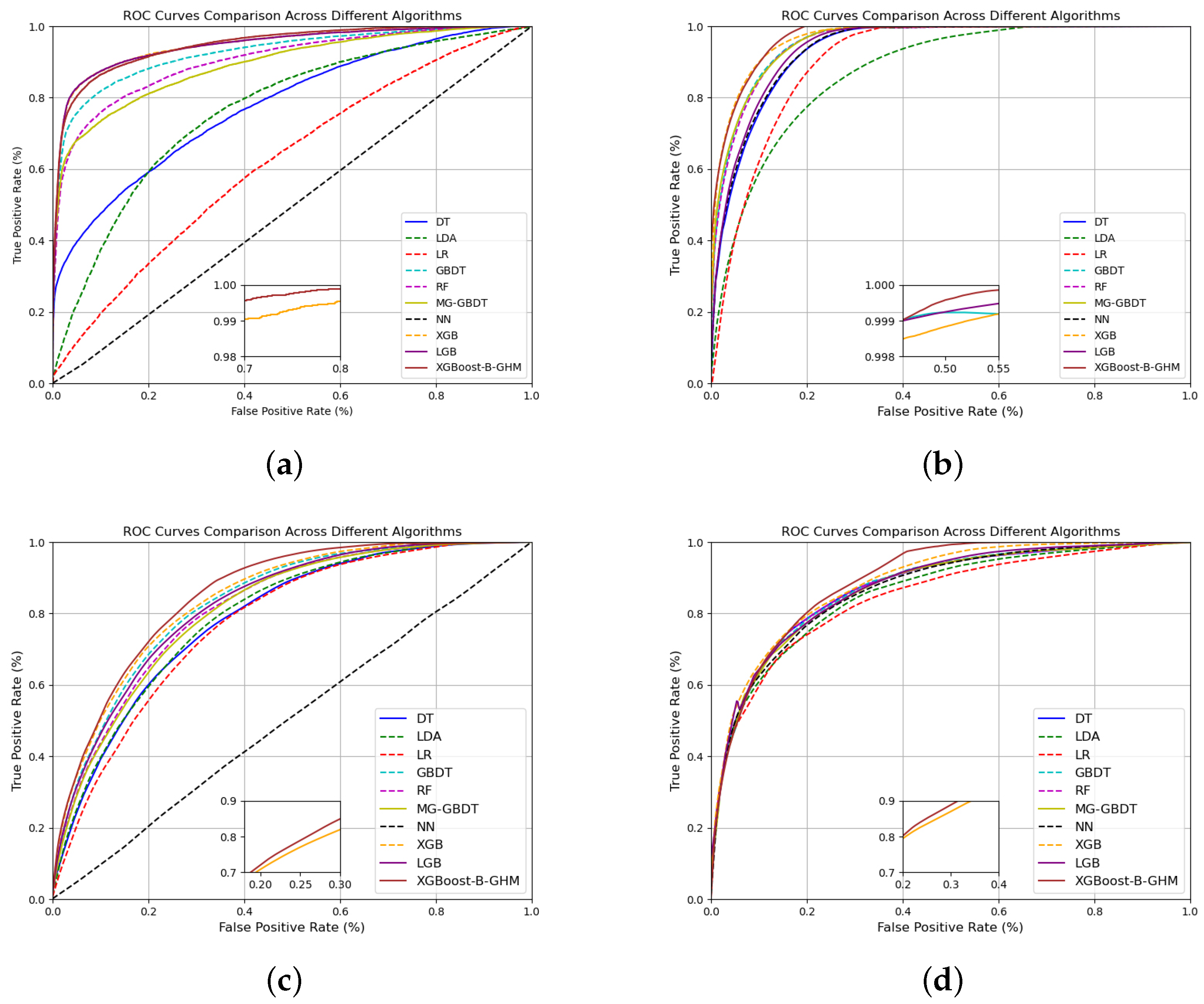
Figure 4 shows the ROC curves of different credit scoring models on four large datasets: Bankfear, Fannie, Give, and LC. In Figure 4, it is obvious to notice that the XGBoost-B-GHM outperforms any of the other models on all four large datasets, especially on LC. Upon comparing the fine-grained visualization, it becomes evident that the ROC curve convergence rates of the XGB and XGBoost-B-GHM are very similar. The XGB is second only to the XGBoost-B-GHM in classification performance and also shows better classification performance. By comparing with MG-GBDT, we obtain a model with better classification performance than the advanced integrated model proposed by Liu et al. [14], and obtain more accurate results under the premise of inheriting the good interpretability of the hierarchical organization. From Figure 4a,c, we can find that NN has the worst classification performance, which may be caused by the extreme imbalance of data. NN is an instance-based learning method, and its classification decision is completely dependent on the nearest neighbor samples in the training dataset. In imbalanced datasets, the number of samples of a few classes is far less than that of most classes, so the samples of most classes are denser in space and easier to become the nearest neighbors, which makes NN algorithm present a great disadvantage in classification accuracy. Two linear algorithms, LR and LDA, also expose such problems. This means that the performance of the algorithm based on boosting is much superior to that of the baseline model, and it also shows that it is necessary to deal with imbalanced data.

In addition to the ROC, for the sake of further showing the superiority of the model, we selected accuracy score (Acc), precision score (Prec), recall rate (Rec), Brier score (BS), and H-measure (HM) as comparative metrics.

Accuracy is the most basic evaluation index, which describes whether the overall result is predicted correctly or not. The value of accuracy can be calculated by the following formula:

$$Accuarcy=\frac{TP+TN}{TP+FP+TN+FN}.$$

(13)

The higher the accuracy, the better the overall prediction performance of the model. In many studies, accuracy may not be a completely reliable indicator because there is a category imbalance in the dataset. In this study, the GHM loss function is used to deal with the problem of class imbalance, which makes the model pay balanced attention to different classes of samples, thus significantly improving the accuracy value of the model.

Precision and accuracy look similar, but they are completely different concepts. Precision is the percentage of samples that are actually positive when the model predicts positive results. It measures the reliability of the model’s positive results and can be calculated by the following formula:

$$Precison=\frac{TP}{TP+FP}.$$

(14)

The recall rate conveys the probability that the sample is correctly predicted as a positive example among all the samples that are actually positive examples. It measures the probability that the model will predict all the positive examples correctly, and its formula is as follows:

$$Recall=\frac{TP}{TP+FN}.$$

(15)

According to Equations (15) and (17), the higher the accuracy and recall rate, the more superior the predictive capabilities of the model. However, there is often a tradeoff between the two; that is, the improvement in one indicator is often accompanied by the decline in another indicator, so comprehensive consideration is necessary.

Brier score is also a measure of the difference between the algorithm’s predicted value and the true value and is calculated as the mean square error of the probabilistic prediction relative to the test sample, expressed as

$$BrierScore=\frac{1}{N}\sum _{i=1}^N{[\widehat{P}\left(\widehat{y_i}\right|x_i)-I\left(\widehat{y_i}\right|y_i)]}^2,$$

(16)

where N is the number of samples and $I(·)$ denotes the indicator function. Therefore, when the Brier score is small, it means that the distinctiveness between the prediction probability and the actual result is tiny; that is, the prediction of the model is more accurate, and vice versa, that the prediction performance of the model is poor.

Table 4. Performance comparison on Bankfear dataset.

Algorithm	Acc	AUC	Prec	Rec	BS
AdaBoost	0.8432	0.8878	0.9402	0.3577	0.1558
DT	0.8243	0.7781	0.8353	0.3227	0.1336
KNN	0.8057	0.6622	0.7593	0.2646	0.0914
LR	0.7662	0.6210	0.7014	0.0246	0.1762
LDA	0.7761	0.7647	0.5562	0.2271	0.1526
NN	0.8991	0.9188	0.0800	0.6102	0.0800
SVM	0.8854	0.9201	0.0859	0.6185	0.0859
RF	0.8544	0.9038	0.9374	0.4137	0.1020
GBDT	0.8912	0.9259	0.9217	0.5913	0.0824
MG-GBDT	0.8897	0.8932	0.8973	0.6042	0.1106
XGB	0.9216	0.9469	0.9016	0.7516	0.0633
LGB	0.9211	0.9467	0.9026	0.7483	0.0633
XGBoost-B-GHM	0.9298	0.9676	0.9212	0.7652	0.0783

shows the performance comparison of various credit scoring models on the Bankfear dataset. According to Table 4, the XGBoost-B-GHM performs better than the baseline credit scoring models that were mentioned at the beginning of 3.2 in three out of five metrics, and also shows better predictive performance than the advanced models (MG-GBDT, XGB, and LGB). The XGBoost-B-GHM scores closest to 1 on the accuracy, AUC, and precision indicators with higher predictive accuracy and reliability. In addition, due to the tradeoff between precision and recall rate, it is difficult for the same model to reach the highest value in both two indexes. Therefore, although the precision of the XGBoost-B-GHM is not the highest among all the models, it is undoubtedly the best in terms of the comprehensive performance of precision and recall rate. Nevertheless, it is worth mentioning that the XGBoost-B-GHM did not achieve better performance in the BS metric than XGB and LGB. Still, the XGBoost-B-GHM scores better on the BS metric than the other benchmark credit scoring models. Although it performs well in many aspects, it may not be dominant in specific datasets or tasks, which also conforms to the fact that each model has its applicable scenarios and limitations, and the selection and adjustment of hyperparameters still need to be optimized.

In the comparison of fifteen models, LR performed the worst in accuracy, AUC, and recall rate, NN performed the worst in precision, and AdaBoost performed the worst in BS. From this, we can easily find that the predictive efficiency of the benchmark credit scoring model is not very high. Among them, LR and LDA had the worst overall performance. Considering that Bankfear is a large dataset, its sample size is sufficient to support the training of machine learning models, so the problem of sparse data can be excluded. Then, the poor performance of LDA and LR is mainly due to their linear nature, and, secondly, it may be that it ignores the order between words, leading to a certain degree of semantic loss. In addition, compared with more advanced ensemble learning, LDA is not efficient when processing large-scale datasets and cannot fully learn the features of the dataset, thus affecting its prediction accuracy.

Table 5. Performance comparison on LC dataset.

Algorithm	Acc	AUC	Prec	Rec	BS
AdaBoost	0.8820	0.9393	0.7198	0.6730	0.2442
DT	0.8766	0.9362	0.7133	0.6443	0.0815
KNN	0.8156	0.8697	0.5463	0.4673	0.1137
LR	0.8446	0.9050	0.6335	0.5361	0.0997
LDA	0.8415	0.8744	0.6705	0.4146	0.1102
NN	0.8786	0.8884	0.6084	0.3688	0.1091
SVM	0.8260	0.8884	0.6084	0.3688	0.1091
RF	0.8983	0.9554	0.7684	0.7066	0.0687
GBDT	0.9017	0.9569	0.7681	0.7315	0.0673
MG-GBDT	0.9021	0.9577	0.7926	0.6940	0.0665
XGB	0.9034	0.9580	0.7794	0.7238	0.0658
LGB	0.8821	0.9429	0.7285	0.6595	0.0785
XGBoost-B-GHM	0.9146	0.9700	0.8077	0.7547	0.0649

shows the performance comparison of various credit scoring models on the LC dataset. As can be observed from Table 5, the XGBoost-B-GHM achieved the best results in every evaluation indicator. This surprising result, on the one hand, shows that the parameter settings on the LC dataset are almost optimal, and, on the other hand, it shows a significant improvement in the classification performance compared to its base model. In addition, MG-GBDT and XGB also show good classification and prediction performance. Because XGB’s training complexity is lower than the XGBoost-B-GHM, it can be used as an effective alternative to the XGBoost-B-GHM. The results shown in Table 5 show that KNN is almost the worst-performing model on the LC dataset, which is similar but not identical to the results on the Bankfear dataset. As with ROC curves, extremely imbalanced datasets make KNN poor for classification and prediction performance.

Table 6. Performance comparison on Fannie dataset.

Algorithm	Acc	AUC	Prec	Rec	BS
AdaBoost	0.9215	0.8249	0.4353	0.0630	0.0806
DT	0.9240	0.7893	0.6098	0.0089	0.0641
KNN	0.9221	0.5113	0.0545	0.0007	0.0848
LR	0.9238	0.7753	0.5200	0.0046	0.0654
LDA	0.9236	0.7943	0.4859	0.0245	0.0641
NN	0.8658	0.5049	0.0762	0.0633	0.1149
SVM	0.9230	0.5017	0	0	0.0736
RF	0.9244	0.8170	0.6375	0.0181	0.0621
GBDT	0.9246	0.8319	0.5544	0.0579	0.0610
MG-GBDT	0.9241	0.8136	0.8000	0.0057	0.0631
XGB	0.9223	0.8431	0.5913	0.0423	0.0613
LGB	0.9219	0.8264	0.7750	0.0107	0.0631
XGBoost-B-GHM	0.9268	0.8864	0.7042	0.1204	0.0770

displays the performance comparison of various credit scoring models on the Fannie dataset. As can be observed from Table 6, compared with the performance of MG-GBDT, XGB, and LGB, the overall performance of the XGBoost-B-GHM has been greatly improved, especially in accuracy, AUC, and recall rate, and the XGBoost-B-GHM has achieved the best results. In the precision score, MG-GBDT is better than the XGBoost-B-GHM, and, in the Brier score, all the models except AdaBoost, KNN, and NN are better than the new model. This result may be related to the characteristics of the Fannie dataset. Boruta is an effective method for feature selection, but it may remove some features that are critical to the model performance under different hyperparameter settings for different datasets. At the same time, hyperparameter adjustment is also crucial. The Brier score can be reduced by tuning the parameters without affecting the overall performance.

Table 7. Performance comparison on Give dataset.

Algorithm	Acc	AUC	Prec	Rec	BS
AdaBoost	0.9372	0.8649	0.5927	0.2033	0.2334
DT	0.9353	0.8573	0.5549	0.1808	0.0502
KNN	0.9332	0.6676	0.7692	0.0067	0.0605
LR	0.9003	0.8457	0.3353	0.1755	0.0942
LDA	0.9379	0.8565	0.5514	0.2835	0.0532
NN	0.9373	0.8677	0.5854	0.2151	0.0493
SVM	0.9329	0.5003	0	0	0.0679
RF	0.9399	0.8725	0.6520	0.1809	0.0475
GBDT	0.9392	0.8734	0.6071	0.2073	0.0476
MG-GBDT	0.9353	0.8711	0.7333	0.0224	0.0507
XGB	0.9350	0.8867	0.9143	0.0319	0.0499
LGB	0.9402	0.8765	0.6918	0.1922	0.0473
XGBoost-B-GHM	0.9433	0.9163	0.7325	0.2400	0.0723

reveals the performance comparison of various credit scoring models on the Give dataset. Similar in some respects to the results of the Bankfear and Fannie datasets, the XGBoost-B-GHM presents the best results on three metrics, namely accuracy score, AUC, and recall rate. On precision score, XGB is significantly higher than any of the other models, and LGB’s Brier score is better than the XGBoost-B-GHM. XGB is 25% more precise than the XGBoost-B-GHM, but the recall rate is 86.7% lower than the XGBoost-B-GHM, which is a considerable gap. It can be observed that the new model proposed in this paper, namely the XGBoost-B-GHM, demonstrates great improvement over the original XGBoost algorithm. Considering other performance aspects, LGB may be an effective alternative to the XGBoost-B-GHM.

4.2. Discussion on Performance of Credit Scoring Models

In general, the XGBoost-B-GHM achieves relatively optimal performance on the four datasets, which can be attributed to the characteristics and advantages of the model in the following aspects. Firstly, Boruta greatly simplifies the dataset by automatically identifying and selecting the important features, eliminating irrelevant and redundant features, and enabling the subsequent model training to be more focused on the key features. Therefore, using Boruta can not only improve the training efficiency of the model but also enhance the degree of accuracy in model predictions. In addition, Boruta ensures the stability and reliability of the selected features by comparing the importance of the original and random features. Secondly, using XGBoost as the main model also contributes to the overall excellent performance of the model. XGBoost combines the advantages of the gradient lifting decision tree algorithm and introduces regular term and parallel computing techniques so that the model can maintain a rapid training speed while preventing overfitting and improving the generalization ability. Moreover, XGBoost provides feature importance ranking, further enhancing the interpretability of the model. Thirdly, embedding the GHM loss function into the XGBoost model further improves the prediction accuracy of the model by assigning different weights to samples with different difficulty levels. It is precisely because the XGBoost-B-GHM combines many advantages to show the best performance in the comparison of a large number of models that the XGBoost-B-GHM can not only be applied to a variety of complex datasets and tasks but also has high prediction accuracy, stability, interpretability, and generalization ability, and has a wide range of application prospects in practical applications.

4.3. AUC and Loss Curves of Integration Models

Due to the competitive performance of several boosting models on ROC curves, we further compared the AUC and loss curves of the MG-GBDT, XGB, LGB, and XGBoost-B-GHM. The AUC considers the performance of the model under all the possible thresholds, providing a more complete picture of the classification capability of the model than the accuracy or recall rate under a single threshold. Moreover, in the process of adjusting the parameters, it is very important to observe the changes in the various parameters during training, so the validation loss function is introduced into our visualization. 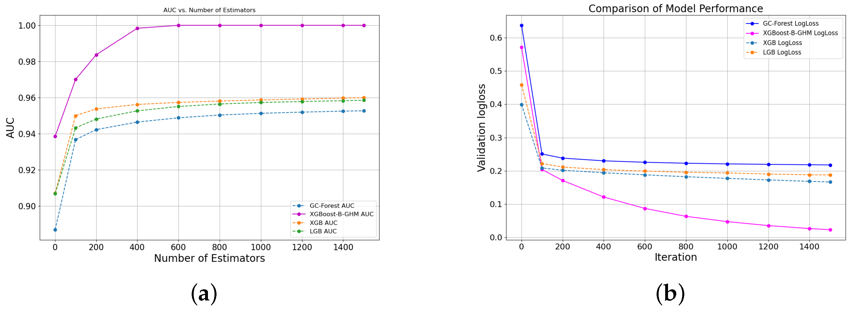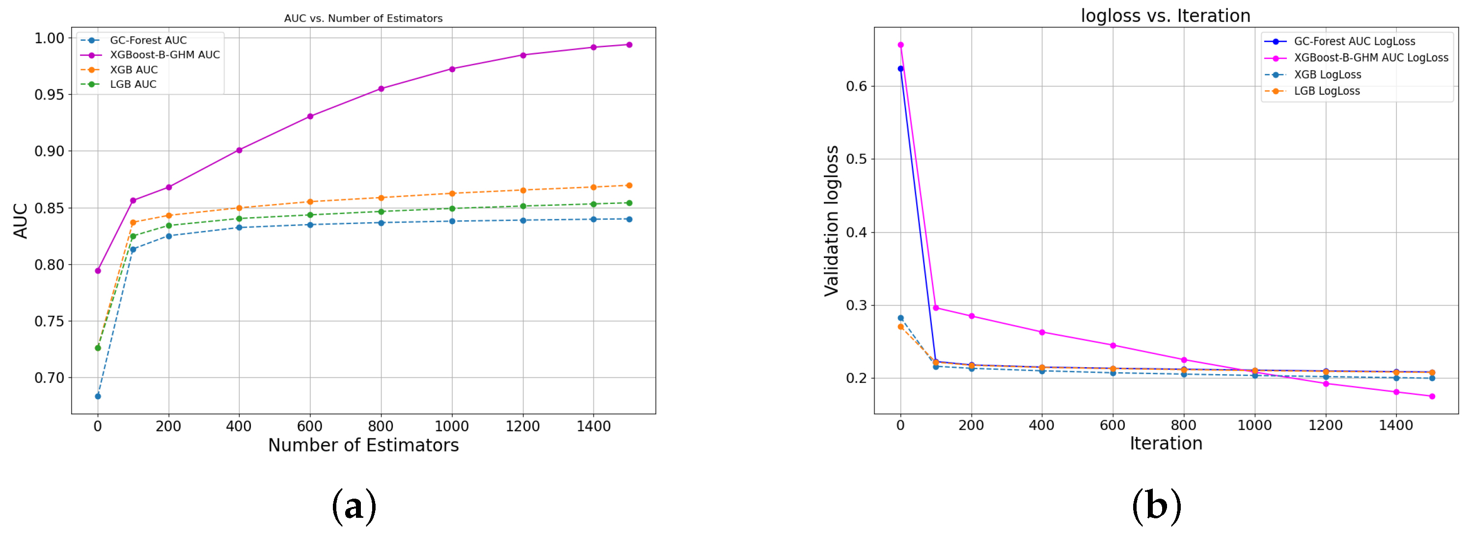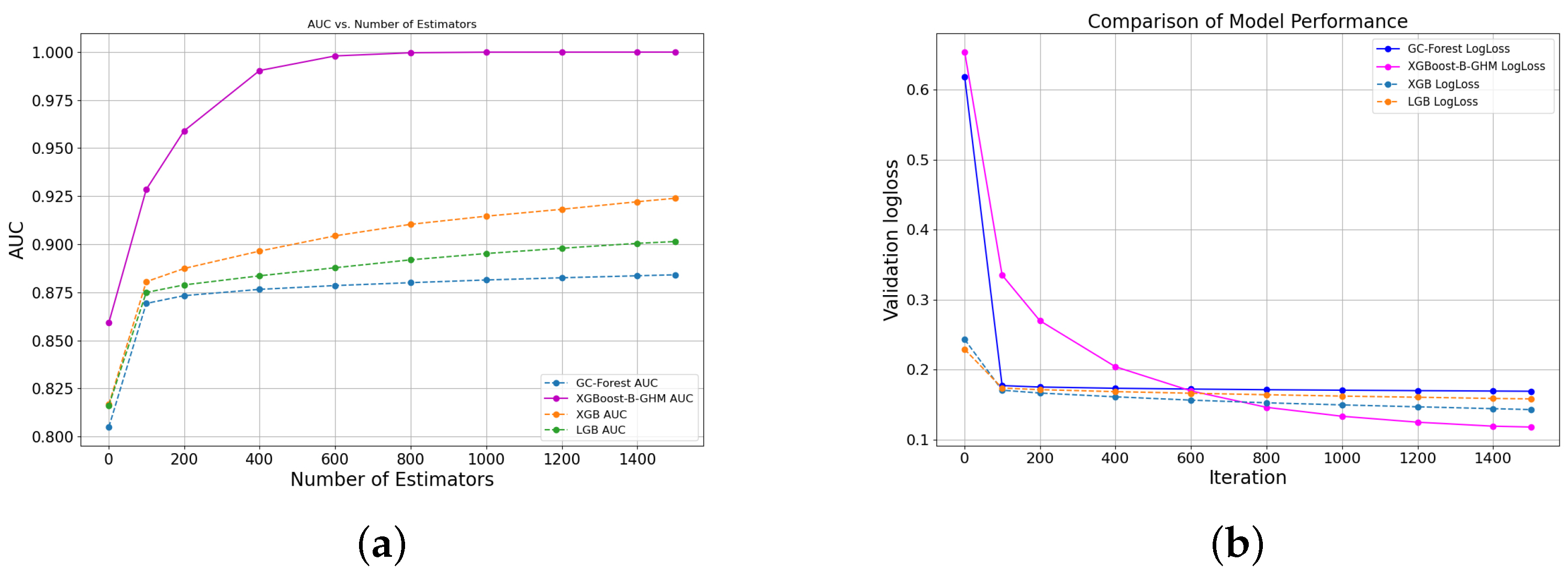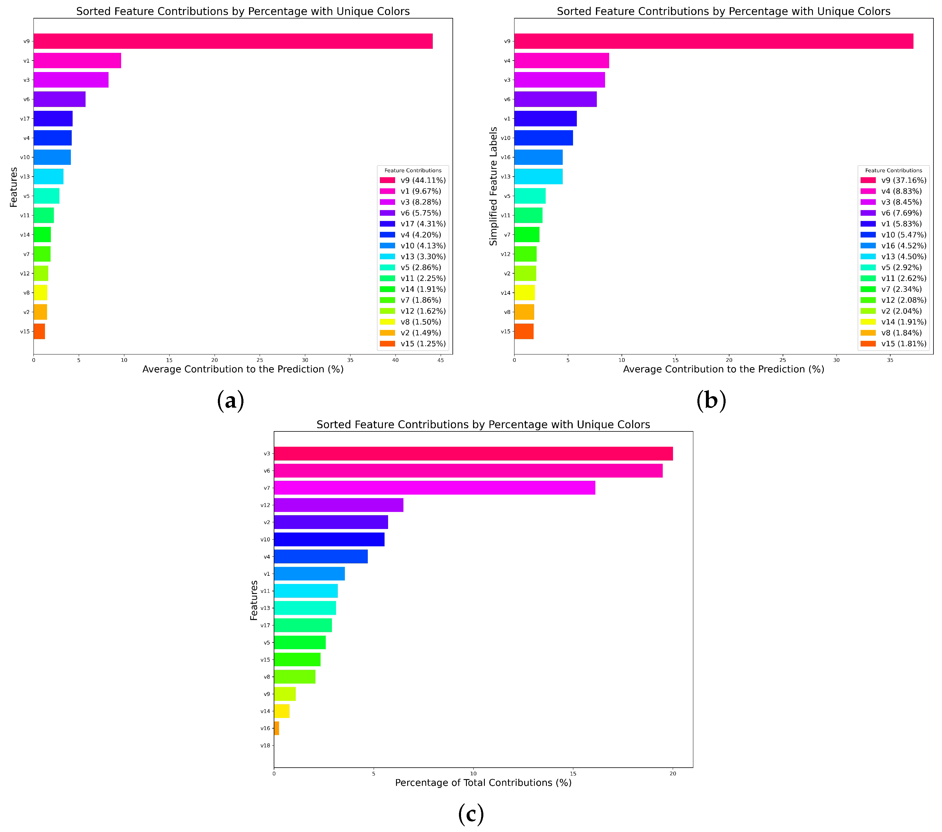Figure 5, Figure 6, Figure 7 and Figure 8 show the AUC and loss curves of four advanced integration models on four credit score datasets, where GC-Forest represents the core algorithm of the MG-GBDT model and Boruta-XGB represents the core algorithm of the XGBoost-B-GHM.

Figure 5 shows the AUC curve and the loss curve on the LC dataset. The overall trend between the two curves and the gap between the other models are similar to the performance on the Bankfear dataset, but the performance on the LC dataset is even better. The AUC curve of the XGBoost-B-GHM converges to 1 after 400 iterations. The performance of LGB and XGB is similar, while XGB is slightly higher than LGB. Both of them converge to 0.96 after 400 iterations, and GC-Forest has the worst performance. In the comparison of the ensemble algorithm loss curves shown in Figure 5b, the XGBoost-B-GHM has the smallest prediction error, and the performance of XGB and LGB is opposite to that of their AUC curves, which indicates that the XGBoost-B-GHM is the optimal approach for the credit scoring of an LC dataset.

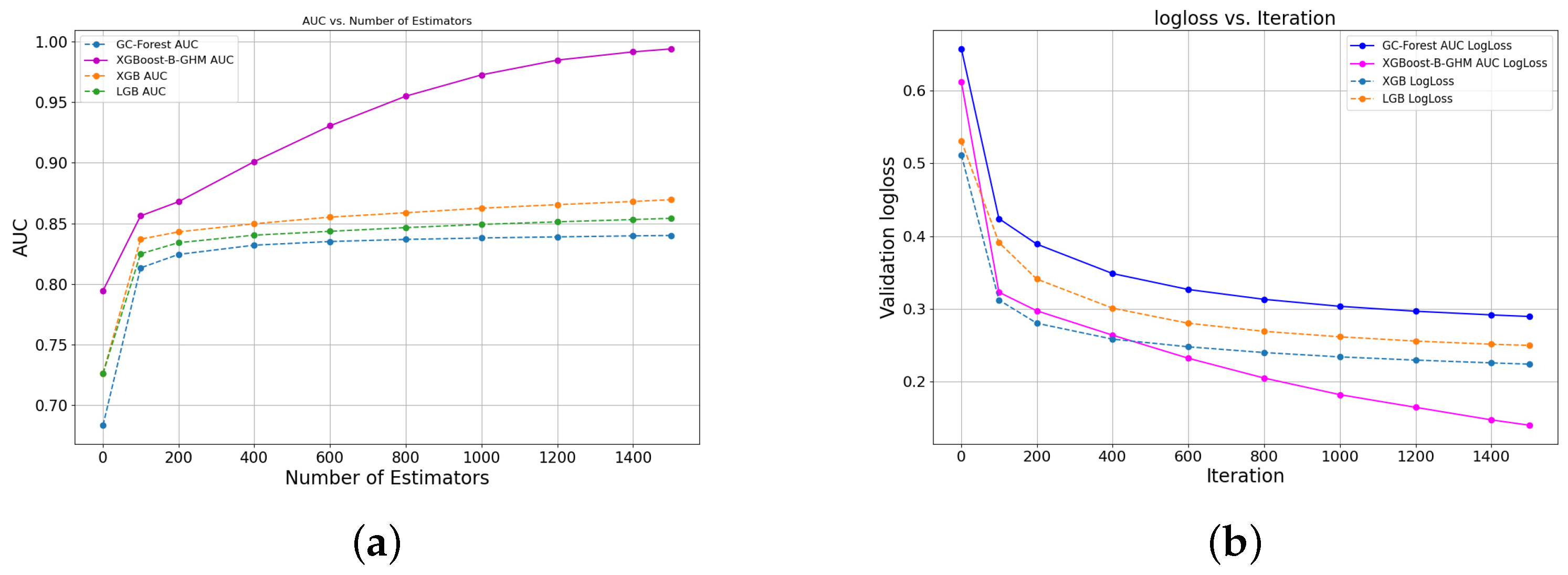
We can obtain the following information from Figure 6. Figure 6a shows the AUC curves of the four ensemble methods on the Bankfear dataset; Figure 6b shows the loss curves of the four ensemble methods on the Bankfear dataset. It can be clearly observed that, after 200 iterations, the slope of the AUC curve of the XGBoost-B-GHM increases significantly, showing a strong performance far superior to the other three ensemble models. After 400 iterations, the prediction error of the XGBoost-B-GHM decreased significantly, but, different from the other three integrated models, the loss curve of the new model still showed a downward trend after 1000 iterations, and more iterations were needed to stabilize it. After 1400 iterations, a stable trend appeared.

The plot in Figure 7 presents the AUC curve and the loss curve on the Fannie dataset. In Figure 7a, the optimal AUC curve on the Fannie dataset is still provided by the XGBoost-B-GHM model, and the performance of the other three ensemble models is still the same as before, among which XGB is the best, LGB is second, and GC-Forest is the worst, but there is a large gap between the three models and the XGBoost-B-GHM. As depicted in Figure 7b, when the number of iterations is small, the prediction error of the XGBoost-B-GHM is large, and, after 1000 iterations, it obtains the optimal convergence loss. In addition, the convergence values of the loss curves of LGB and GC-Forest are similar, and it can be observed from the fine-grained comparison plot that the predicted loss of LGB is slightly lower than that of GC-Forest.

Figure 8 shows the AUC curve and the loss curve on the Give dataset. From Figure 8a,b, we can find that it is still the XGBoost-B-GHM that obtains the best convergence AUC and convergence loss. XGB obtained the second-best convergence AUC and loss score, but its AUC performance was still significantly lower than the XGBoost-B-GHM.

On all four datasets, at the beginning of training, the loss value of the XGBoost-B-GHM decreased significantly, indicating that the learning rate was set appropriately and the gradient descent process was underway. After a certain number of iterations, the loss curve of the XGBoost-B-GHM decreases steadily until it becomes stable. On the Give dataset, the prediction error of the XGBoost-B-GHM after 100 iterations is much smaller than that of the other models. On the Bankfear dataset, the prediction error of the XGBoost-B-GHM after 400 iterations is much smaller than that of the other models. After more than 1000 iterations, the prediction error of the proposed model on both the LC and Fannie datasets gradually leveled off. We can also see from Figure 7b and Figure 8b that the loss curves of XGB and LGB are similar because they have the same gradient lifting framework and similar loss functions and optimization objectives. The XGBoost-B-GHM creatively embeds the GHM loss function in XGB with more subtle errors than XGB and LGB, which further validates the excellent performance of the XGB model embedded in GHM in handling imbalanced data.

4.4. Comparison with Standard Methods

4.4.1. Comparison of Different Feature Selection Methods

The main feature selection methods are divided into three types, respectively filter methods, wrapper methods, and embedded methods [41]. In order to better compare our models, the most popular least absolute shrinkage and selection operator (LASSO) [42] and RIDGE [43], which are good at dealing with data with multicollinearity, are selected for comparison with Boruta, and the performance comparison of different feature selection methods is shown in

Table 8. Performance comparison of different feature selection models on Bankfear dataset.

Methods	Acc	AUC	Prec	Rec	BS
Boruta	0.9298	0.9676	0.9212	0.7652	0.0783
LASSO	0.9088	0.9407	0.8951	0.6912	0.0958
RIDGE	0.8206	0.8304	0.6809	0.4392	0.1462

,

Table 9. Performance comparison of different feature selection models on LC dataset.

Methods	Acc	AUC	Prec	Rec	BS
Boruta	0.9146	0.9700	0.8077	0.7547	0.0649
LASSO	0.7815	0.7155	0.5892	0.0942	0.1936
RIDGE	0.8002	0.7048	0.5552	0.0303	0.1885

,

Table 10. Performance comparison of different feature selection models on Fannie dataset.

Methods	Acc	AUC	Prec	Rec	BS
Boruta	0.9268	0.8864	0.7042	0.1204	0.0770
LASSO	0.9238	0.8511	0.6233	0.0774	0.1015
RIDGE	0.9213	0.7375	1.0	0.0007	0.1015

and

Table 11. Performance comparison of different feature selection models on Give dataset.

Methods	Acc	AUC	Prec	Rec	BS
Boruta	0.9433	0.9163	0.7325	0.2400	0.0723
LASSO	0.9386	0.8936	0.6156	0.2201	0.1040
RIDGE	0.8472	0.8472	0.6168	0.2052	0.1476

. In these comparisons, we merely replace the different feature selection methods while keeping the other algorithms unchanged.

Table 8 shows the performance comparison of different feature selection methods on the Bankfear dataset. Table 9 shows the performance comparison of different feature selection methods on the LC dataset. Table 10 shows the performance comparison of different feature selection methods on the Fannie dataset. Table 11 shows the performance comparison of different feature selection methods on the Give dataset. It is easy to find that Boruta performs best in all five metrics, and it shows a significant advantage across these metrics, especially when compared to RIDGE. In fact, RIDGE itself does not perform variable selection because it fails to produce a sparse model and prefers a dense solution [44]. Further, la Tour et al. [45] generalized ridge regression to banded ridge regression to achieve more accurate and interpretable feature space selection. Unlike RIDGE, which performs L2 regularization, LASSO performs L1 regularization, which helps to generate a sparse weight matrix that can in turn be used for feature selection. One possible explanation for the difference in performance between RIDGE and LASSO may be the different regularization methods used. The comparison results between Boruta and these two regularization methods further confirm the superiority of the XGBoost-B-GHM.

4.4.2. Comparison of Different Machine Learning Methods

After comparing different feature selection methods, we also need to know whether it is optimal to use XGBoost as the core algorithm. Based on the four datasets, we replace XGBoost with standard models such as RF and LR, respectively, in an attempt to verify the superiority of XGBoost.

Table 12. Performance comparison of machine learning methods on Bankfear dataset.

Methods	Acc	AUC	Prec	Rec	BS
XGBoost	0.9298	0.9676	0.9212	0.7652	0.0783
RF	0.8145	0.7470	0.9252	0.2364	0.1438
LR	0.7638	0.6123	0.6667	0.0065	0.1786

,

Table 13. Performance comparison of machine learning methods on LC dataset.

Methods	Acc	AUC	Prec	Rec	BS
XGBoost	0.9146	0.9700	0.8077	0.7547	0.0649
RF	0.8943	0.9598	0.7898	0.7251	0.0716
LR	0.8833	0.9447	0.7138	0.8069	0.0785

,

Table 14. Performance comparison of machine learning methods on Fannie dataset.

Methods	Acc	AUC	Prec	Rec	BS
XGBoost	0.9268	0.8864	0.7042	0.1204	0.0770
RF	0.9047	0.5654	0.1469	0.0445	0.0874
LR	0.9215	0.6705	0.0000	0.0000	0.0711

and

Table 15. Performance comparison of machine learning methods on Give dataset.

Methods	Acc	AUC	Prec	Rec	BS
XGBoost	0.9433	0.9163	0.7325	0.2400	0.0723
RF	0.9331	0.7898	0.8000	0.0119	0.0567
LR	0.9309	0.7813	0.3125	0.0198	0.0583

show the performance of the different machine learning methods on the four datasets. Table 12 and Table 15 show the performance of the individual models on the Bankfear and Give datasets, respectively, in which XGBoost achieves the best scores on four of the five metrics, except precision. Table 13 shows XGBoost’s best performance on Acc, AUC, Prec, and BS on the LC dataset. Although XGBoost’s recall rate is not the highest, as mentioned above, precision and recall rate need to be considered together, so XGBoost still achieves the best performance overall. The performance on Fannie dataset, which is presented in Table 14, is somewhat different from the performance on the other three datasets, but arguably better. The BS score is second only to the LR model, and all the other indicators reach the best of the three models. When we do not control the two variables, feature selection and loss function, RF and LR perform much worse than the XGBoost-B-GHM. When we keep the feature selection method and loss function of RF and LR as the same as the XGBoost-B-GHM, and only change the main machine learning model, although the performance of RF and LR is still worse than that of the XGBoost-B-GHM, the performance has been greatly improved compared with the original model without controlling variables. This can also illustrate the superiority of using Boruta for feature selection and embedding GHM loss function in this paper from another perspective.

4.5. Model Interpretability and Fairness

4.5.1. Model Interpretability

Figure 9 highlights the feature importance scores calculated on the Fannie datasets. Figure 9a displays the feature importance score of the model without Boruta for feature selection, Figure 9b shows the feature importance score of the model with Boruta for feature selection, and Figure 9c shows the importance score of the input features of the Fannie dataset.

Table 16. Feature description of the Fannie dataset.

Variable	Feature Name	Description
$V_1$	Original interest rate	The initial or starting interest rate that is set for a loan.
$V_2$	Original UPB	Principle amount
$V_3$	Original loan term	Original loan term
$V_4$	Original loan-to value (LTV)	The loan-to-value ratio at the initial stage of loan issuance.
$V_5$	Original combined loan-to-value (CTLV)	The combined loan-to-value ratio at the initial stage of loan issuance
$V_6$	Number of borrowers	Number of borrowers
$V_7$	Original debt to income ratio	The ratio of debt to income at the beginning of the loan.
$V_8$	Number of units	Number of units
$V_9$	MI	Mortgage Insurance
$V_{10}$	Min credit score	The borrower’s credit score
$V_{11}$	Original channel	Origination channel.
$V_{12}$	Seller name	Seller name
$V_{13}$	First time home buyer indicator	First time home buyer indicator
$V_{14}$	Loan purpose	Loan purpose (such as buy a car or house)
$V_{15}$	Property type	The area where the property is secured by the mortgage.
$V_{16}$	Occupancy type	The type of occupancy
$V_{17}$	Property state	Property state
$V_{18}$	Relocation mortgage indicator	Relocation mortgage indicator

presents the corresponding characteristic descriptions on the Fannie dataset. From Figure 9c and Table 16, we can come to the conclusion that the original loan term contributes most to the prediction. In addition to $V_3$, the number of borrowers and original debt to income ratio rank in the top three. In addition, $V_{12}$, $V_2$, $V_{10}$, and $V_4$ are also borrower characteristics that should be considered in credit granting.

To further verify the global interpretability of the XGBoost-B-GHM, the feature importance scores on the Give dataset are quantified and displayed in Figure 10. Figure 10a shows the feature importance score of the model without Boruta for feature selection, Figure 10b shows the feature importance score of the model with Boruta for feature selection, and Figure 10c shows the importance score of the input features of Give dataset.

Table 17. Feature description of the Give dataset.

Variable	Feature Name	Description
$V_1$	SeriousDlqin2yrs	Serious overdue payments within two years.
$V_2$	RevolvingUtilizationOfUnsecuredLined	Total balance on credit card except real estate and car loans/credit limit.
$V_3$	age	The age of borrower
$V_4$	NumberOfTime3059DaysPastDueNotWorse	Borrowers are 30–59 days overdue, but no worse in the last two years.
$V_5$	DebtRatio	Debt radio
$V_6$	MonthlyIncome	Monthly income
$V_7$	NumberOfOpenCreditLinesAndLoans	The number of open loans and lines of credit.
$V_8$	NumberOfTimes90DaysLate	Number of times the borrower is 90 days or more past due on payments.
$V_9$	NumberRealEstateLoansOrLines	The amount of real estate loans
$V_{10}$	NumberOfTime6089DaysPastDueNotWorse	Borrowers are 60–89 days overdue, but no worse in the last two years.

presents the corresponding characteristic descriptions on the Give dataset. From Figure 10c and Table 17, it can be found that the serious overdue payments within two years contribute the most. Among the several features with high feature importance scores, $V_1$ scores far higher than the others, contributing an average of 35% to the final prediction. This shows that the historical credit status is a very important factor in the process of credit investigation. The two features following $V_1$ are age and the number of open loans and credit lines, which is consistent with the actual credit granting situation; therefore, it can be considered that the XGBoost-B-GHM model has high global interpretability.

4.5.2. A Discussion of Model Fairness

The model constructed in this paper is intended to be used for credit scoring of borrowers. Similarly, models play a crucial role in everyday decision making. Therefore, in order to guarantee that the model can provide fair results for everyone, the model creation process also requires fairness. In addition, the international artificial intelligence regulations also clearly stipulate that artificial intelligence models based on machine learning need to be fair [46]. Each model builder has a responsibility to detect and mitigate fairness issues. In this paper, we constructed the confusion matrix shown in Table 3, which clearly defines harms and benefits. Moreover, we evaluated the interpretability of the model by calculating feature importance scores, resulting in an interpretable and robust model. Further evaluation and improving the fairness of machine learning models can be achieved by using Fairlearn, a Python package [47]. However, we did not use this package in our experiment, and we will further consider the fairness in our future research. We also hope that more scholars can carry out research in this regard.

4.6. Significance Test

For the sake of testing whether there are differences in the performance comparison results of each group of data in the experiment and whether the differences are significant, a statistical significance test is conducted. Due to the differences between non-parametric statistical testing methods and parametric hypothesis testing methods, the non-parametric statistical significance testing technique Friedman test was adopted because we could not make simple assumptions about the population distribution in large datasets. The statistics of Friedman’s test can be calculated as follows:

$${\chi }_F^2=\frac{12N}{k(k+1)}[\sum _{j=1}^k{r}_j^2-\frac{k{(k+1)}^2}{4}],$$

(17)

where $r_j$ denotes the mean of the ranks of the j-th method, k denotes the number of methods involved, and N denotes the number of datasets or experiments involved. Friedman statistics obey the chi-squared distribution of k-1 degrees of freedom, and they are calculated to 29.8479 and the p-value of the statistics is calculated to 0.0029, which are shown in

Table 18. Friedman test.

Algorithm	Friedman Statistic	p-Value	Null Hypothesis
XGBoost-B-GHM	29.8479	0.0029	Reject

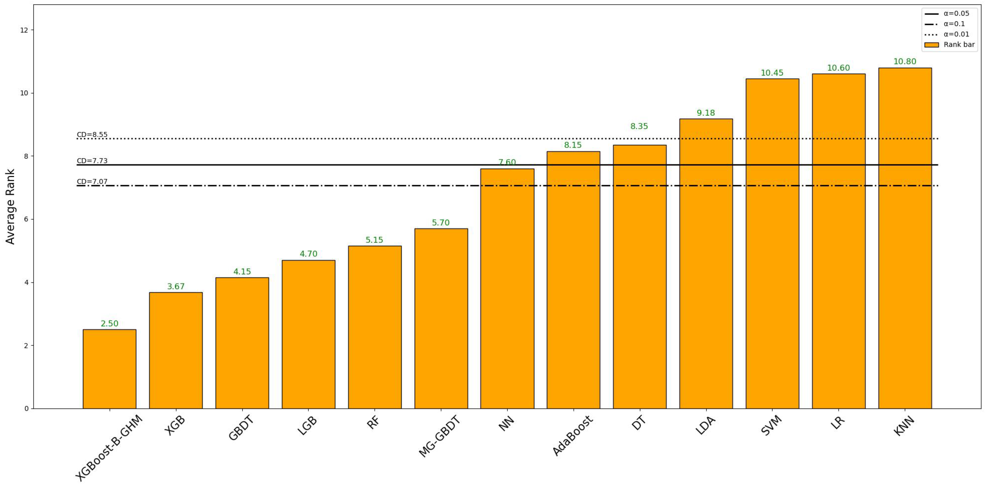
. This P-value is less than the significance level (set $\alpha$ to 0.1, 0.05, and 0.01, respectively, for calculation), so the null hypothesis can be rejected and the scores of each metric are considered to be significantly different. Due to the condition that the null hypothesis is rejected, the Nemenyi follow-up test will be performed. In the Nemenyi test, two methods are said to be significantly different if the mean rank difference between them reaches a critical difference (CD). The calculation of CD can be expressed by the following formula:

$$CD=q_{\alpha }\sqrt{\frac{k(k+1)}{6N}}$$

(18)

In the above formula, $\alpha$ represents the significance level. In this experiment, we set the value of $\alpha$ as 0.1, 0.05, and 0.01, respectively, to calculate CD at different significance levels, and $q_{\alpha }$ is the constant obtained by looking up the table and $q_{0.05}$ = 2.9480. So far, we can calculate the CD values at the corresponding significance level as 7.07, 7.73, and 8.55 according to Equation (18).

Figure 11 depicts the average ranking of all the metrics on the four datasets for all the credit evaluation models tested in this paper. The three horizontal lines from top to bottom show the value of CD calculated with significance levels of 0.01, 0.5, and 0.1, respectively. We can see from Figure 11 that the average ranking of the XGBoost-B-GHM is 2.5, which is the highest among all 13 models. The experimental results show that the performance of the ensemble model is much higher than that of the single model, and the tree structure is more suitable for imbalanced data, and its performance improvement is significant. The XGB model performs better than LGB on imbalanced data and is a reliable alternative to the XGBoost-B-GHM. SVM and LR, which were originally linear classifiers, have shown poor performance on imbalanced datasets. KNN ranks the lowest, indicating that it may not be a model that can be used on imbalanced data, although it may not perform as poorly on other datasets.

5. Discussion

5.1. Advantages of the Proposed Method

The research offers several notable strengths. Firstly, the development of the XGBoost-B-GHM model, which combines feature selection through the Boruta algorithm and the GHM loss function, represents an innovative approach to credit scoring. This ensemble model effectively addresses the common challenges in credit evaluation, such as dealing with redundant data features and imbalanced sample distributions. By incorporating the Boruta algorithm, the model achieves dimensionality reduction and noise mitigation, improving its generalization capabilities. The GHM loss function, when integrated into XGBoost, enhances the model’s performance by focusing on samples that are harder to classify, thereby optimizing its classification and prediction abilities. Moreover, the paper demonstrates the superiority of the proposed method over the established techniques through comparative experiments conducted on extensive datasets. It showcases the model’s capability to efficiently extract relevant features and improve the overall performance in credit scoring tasks. The use of decision trees within the ensemble framework is advantageous due to their interpretability, which facilitates understanding and trust in the model’s decisions.

5.2. Limitations and Expectations

However, despite some advancements, the study also presents certain limitations. While the paper highlights the interpretability of the XGBoost-B-GHM model, it acknowledges the ongoing challenge of ensuring fairness in model outcomes. Model fairness is critical in credit scoring applications as decisions can significantly impact individuals’ lives. We admit that the fairness concerns have not been fully addressed in our current work, and we plan to explore this field further in future studies. This implies that potential biases in the model’s predictions, which could result from inherent biases in the data or algorithm design, might still exist and require careful examination. Additionally, the research does not delve deeply into the specifics of how the model would perform across various types of datasets. Although the experiments are conducted on sizable datasets, the applicability of the model to smaller or differently structured datasets remains unexplored. This could limit the model’s adaptability to different credit scoring scenarios, particularly in cases where the data availability is constrained. The limitations concerning model fairness, generalizability, and operational costs should be considered and addressed in subsequent research to ensure that the model can be reliably deployed in diverse financial environments.

6. Conclusions

As an important part of financial risk management, credit scoring is of paramount importance to evaluate the credit status of borrowers, optimize the allocation of credit resources, and enhance the stability of financial markets. Therefore, it is particularly important to build an efficient and rigorous credit scoring model. In the field of credit scoring, the application of deep learning technology is gradually showing its unique advantages and potential. Compared with the traditional statistical methods and machine learning models, or even some common ensemble models, deep learning is better able to cope with complex and high-dimensional data, automatically learn and extract useful features from the data, and obtain models with stronger accuracy and efficiency regarding credit assessment.

Based on the deep study of the application of deep learning in the field of credit evaluation, this paper proposes an XGBoost ensemble model based on Boruta feature selection and GHM loss function optimization. The model combines the advantages of deep learning in feature extraction and model optimization while using the GHM loss function to overcome data imbalance barriers, which greatly improves the generalization ability of the model. Through a comprehensive analysis of four large credit scoring datasets, we validate the model’s superior performance in the credit scoring task. The experimental results show that the model is significantly better than the traditional models in accuracy, recall rate, AUC, and other key evaluation indicators. This supports the effectiveness and practicability of deep learning technology in the field of credit scoring, and also provides new ideas and methods for future research.

Although the XGBoost-B-GHM model has excellent performance in prediction accuracy and generalization ability, there are still some shortcomings in this study. First, the adjustment and optimization of model parameters involve a complex and time-consuming process. Although the model has been optimized and relatively optimal parameters have been selected in this paper, there may still be some factors that have not been fully considered. The future research could further explore methods for model optimization, such as using automated machine learning techniques [48] to simplify the parameter adjustment process and improve the efficiency of the model. Second, the interpretability of deep learning models is relatively weak. Although the model is excellent in performance, it is difficult to directly explain the inner workings of the model, which makes the model limited by a certain degree of trust in its practical applications. In the future, methods to enhance the model interpretability can be further explored, such as the introduction of multi-dimensional visualization [49] components. In the future, as deep learning technologies continue to develop and improve, we except to see more innovative applications and research results emerge in the field of credit scoring.