Abstract
This research aims to study a real-world example of the unrelated parallel machine scheduling problem (UPMSP), considering job-splitting, inventories, shortage, and resource constraints. Since the nature of the studied optimization problem is NP-hard, we applied a metaheuristic algorithm named Grey Wolf Optimizer (GWO). The novelty of this study is fourfold. First, the model tackles the inventory problem along with the shortage amount to avoid the late fee. Second, due to the popularity of minimizing completion time (Makespan), each job is divided into small parts to be operated on various machines. Third, renewable resources are included to ensure the feasibility of the production process. Fourth, a mixed-integer linear programming formulation and the solution methodology are developed. To feed the metaheuristic algorithm with an initial viable solution, a heuristic algorithm is also fabricated. Also, the discrete version of the GWO algorithm for this specific problem is proposed to obtain the results. Our results confirmed that our proposed discrete GWO algorithm could efficiently solve a real case study in a timely manner. Finally, future research threads are suggested for academic and industrial communities.
1. Introduction
In today’s manufacturing systems, producing goods based on their due dates and priorities is a complex decision problem that needs to be taken into consideration to help manufacturers deliver the products to their customers in a timely manner. The parallel machine scheduling problem (PMSP) is one kind of complex problem that has been widely applied to produce goods in a timely manner and avoid late deliveries. This paper studies a real problem that exists in Bronze Industrial Manufacturing Company (BIMC) in Iran, which produces different parts for major car manufacturers such as Renault and Peugeot. The problem description is to minimize the completion times of all jobs over existing machines (Makespan) while inventories, shortages, resource constraints, job splitting, and machine eligibility are considered. Also, each job has a distinct due date and is split into different sub-jobs that can be processed on different unrelated parallel machines, which vary in terms of speed, resource consumption, productivity, and eligibility. The sequence-dependent setup time is another critical parameter that plays a significant role in this manner.
This study pursues improving the production planning of BIMC by proposing a new formulation of the unrelated parallel machine scheduling problem (UPMSP). The proposed model of this study has novelty due to the following contributions. First, the model tackles the inventory problem along with the shortage amount to avoid late fees. Second, each job is split into sub-parts to be completed on different machines. Third, renewable resources, including cranes, workers, and lift trucks, are integrated to guarantee the feasibility of the solution. Our goal is to maximize productivity by minimizing the completion time of all jobs, which is the most common optimization problem in UPMSP so that we can produce all parts of each job as quickly as possible with the least amount of inventory. Also, the proposed model is coded using a metaheuristic algorithm called Grey Wolf Optimizer (GWO), proposed by Mirjalili et al. [1], due to the NP-hardness nature of the model to provide feasible solutions to the decision makers (DMs). Then, the coding package becomes a part of the manufacturer’s expert and intelligent production system.
Continuing with this study, we will follow the following structure: In the next section, we will cover past studies in PMSP. In Section 3, we will dive into constructing a model and developing a metaheuristic algorithm in Section 4. The results will be discussed in Section 5. Lastly, the conclusions and future research directions are provided in Section 6.
2. Literature Review
The parallel machine scheduling problem has been widely investigated by many studies during the last few decades [2,3,4]. For instance, Allahverdi et al. [5] classified scheduling problems according to shop environments such as single machines, parallel machines, flow shops, job shops, and open shops. Similarly, Cheng et al. [6] summarized various types of machine scheduling problems (MSPs) based on different approaches, including identical parallel machine scheduling where a job should be processed on any identical machine with the same speed, uniform parallel machine scheduling where jobs can be produced on any machine with different speed factors in fixed ratios with each other, and unrelated parallel machine scheduling where each job can be processed on a set of specified machines with varied speed. Also, we have collected past studies conducted on three types of MSPs which are shown in Table 1. In the following paragraphs, we will discuss these three problems in terms of mathematical modeling, solution methodology, constraints, and optimization criterion.

Table 1.
Summarizing the PMSPs with/without splitting the jobs.
Various solution methodologies are applied to solve complex problems. For the identical parallel machine scheduling problems, Kim et al. [7] proposed a two-phase heuristic approach to minimize total tardiness. Also, some researchers [9,10,13] applied tabu search, simulated annealing, heuristic, and iterated greedy-based meta-heuristic algorithm to minimize the total tardiness of their proposed models. Some other researchers have considered minimizing the total completion time of all jobs, which is a commonly known objective function in PMSP. For instance, some [8,9,11,14,35] minimized Makespan in their studies using heuristic, simulated annealing, ant colony optimization, tabu search, and particle swarm optimization algorithms. For the UPMSP, many studies have optimized the objective function by minimizing the total tardiness and completion time, and some others minimized the total energy consumption. Afzalirad and Rezaeian [20] addressed the UPMSP by considering resource constraints, sequence-dependent setup time, various release dates, machine eligibility, and precedence constraints. They utilized two metaheuristic algorithms, including a genetic algorithm and an artificial immune system, to solve the developed integer programming modeling. Similarly, Fanjul-Peyro et al. [21] proposed two mathematical models; the first is based on the literature review of the UPMSP, and the other one is based on the real complex problem of strip packing problems. They could solve the proposed model based on a greedy-based fixing algorithm. Zhang et al. [23] suggested a novel UPMSP in which two factors influence the energy consumption rate of parallel machines: tool changes and corresponding processing speed. Therefore, they optimized two objective functions simultaneously, including completion time and total energy consumption, and then solved them using a heuristic evolutionary algorithm. In another study, Lei et al. [26] optimized both the completion time and total tardiness of the UPMSP as a multi-objective problem. They used an improved artificial bee colony to solve the model. In a recent study conducted by Arık et al. [28], weighted earliness/tardiness is used as an objective function to solve the UPMSP. They proposed a constructive algorithm as a heuristic methodology to tackle the model.
Compared to both UPMSP and IPMSP, some studies were conducted on uniform PMSP. Koulamas et al. [30] utilized a modified longest processing time algorithm for two uniform parallel machines to minimize the completion times of all jobs. The proposed heuristic algorithm could improve the Makespan optimization problem. Yeh et al. [32] minimized the completion times of all jobs, considering resource consumption that should not reach a certain threshold. Alternatively, they utilized several mate-heuristic algorithms, including the genetic algorithm and particle swarm optimization, to find an optimal solution. Zeng et al. [34] presented a model to optimize the total electricity costs as well as the number of machines used for processing all jobs. An iterative search framework based on the proposed insertion procedure is developed to acquire the entire Pareto front of the problem. Lastly, Kaabi et al. [33] proposed a model to minimize the completion time based on deterministic unavailability to solve the uniform UPMSP. A heuristic algorithm was proposed for solving the problem on a large scale.
Splitting the job into subparts has been studied by a few studies in the prior literature. Kim et al. [7] solved the IPMSP by considering job splitting. They could process all parts of one job on parallel machines independently. Similarly, Nait Tahar et al. [8] minimized the total completion time by splitting jobs into different sub-parts. Using job splitting time and a heuristic approach, they could improve the running time of the model by considering more than 6000 examples. In 2011 and 2012, some researchers [9,10] minimized total tardiness by separating all jobs into sub-parts. A few papers studied job splitting on the UPMSP. For instance, Logendran et al. [17] developed a mixed (binary) integer linear programming model aimed at minimizing total tardiness by splitting the job dynamically. Recently, Kim et al. [36] considered job splitting and sequence-dependent setup time simultaneously in IPMSP to present a model and solve it using metaheuristic algorithms. For more information, readers are referred to Table 1.
Many studies have considered the concepts of resource availability, sequence-dependent setup time, and machine eligibility. For the IPMSP, some researchers [8,10] considered sequence-dependent setup times. For the UPMSP, some research considered sequence-dependent setup times, machine eligibility, and resource constraints at the same time [20,27]. While others only considered resource constraints and sequence-dependent setup times [22,24,25]. Only Fanjul-Peyro et al. [21] included resource constraints in their model without paying attention to other constraints as discussed. They limited the resource constraints through the production horizon. Lastly, for uniform PMSP, one study considered sequence-dependent setup times [29], and one other included resource constraints in their proposed model with the objective of minimizing makespan [32].
To the best of the authors’ knowledge, splitting jobs has been studied by many studies. Some other papers studied the effect of resource constraints, machine eligibility, and sequence-dependent setup times at the same time in their model. Also, many studies have been performed on the IPMSP. A few studies looked at the splitting jobs regarding the UPMSP. Therefore, based on what we have discussed, as well as the summarized papers in Table 1, the main contributions of this study are as follows:
- Proposing a new mathematical formulation for the UPMSP with the aim of minimizing the completion time (Makespan) considering job splitting, inventories, and shortages in the production planning horizon, resource constraints, and machine eligibility.
- Developing a heuristic algorithm to produce an initial feasible solution.
- Solving the proposed model using the novel Grey Wolf Optimizer algorithm developed by Mirjalili et al. [1];
- Measuring the performance of the formulation and solution methodology in a real-world production environment, implemented at Bronze Industrial Manufacturing Company (BIMC) in Iran as a decision support system.
3. Mathematical Model
The problem framework is to schedule all jobs over a limited number of machines with different speeds. We aim to minimize the completion time of all jobs in the model, considering inventories, shortages, resource constraints, job splitting, and machine eligibility. Also, some assumptions are considered to establish the underlying boundaries to create a deterministic mathematical model as follows:
- ✓
- The number of unrelated parallel machines and jobs is constant [20,25].
- ✓
- The capability of a machine to complete a job is provided [12].
- ✓
- The Kanban planning of each job is presented based on the days of the week. In other words, the required number of products for each job is known during the production planning phase.
- ✓
- The setup time of the machine is with respect to the changes in the machine’s frames. Moreover, the sequence limitations are provided here.
- ✓
- There are two different working hours and shift duration, six days a week or seven days a week. There are three different working hours have been provided by the BIMC [37].
- ✓
- At the beginning of the planning horizon, the production planner needs to know the inventory levels.
After defining the assumption of the model, we introduce the set, parameters, and variables to build the model of this study. Table 2 shows the notation of the proposed model.

Table 2.
Notation of the proposed model.
The proposed model of this study has been formulated as follows:
The above equation is subject to
The objective function, which is shown in Equation (1), aims to minimize the completion time of all split jobs over different existing machines. Equation (2) displays the inventory balance of each job in different time periods. Equation (3) guarantees that the two variables of inventory and shortage cannot obtain a positive value at the same time, which is written due to the nature of these two defined variables. The eligibility of each split job over all machines is assured by Equation (4). Also, Equation (5) represents the renewable resource constraint of the model, including labor, experts, and cranes. The total number of split jobs that should be produced at the end of the program is shown by Equation (6). Equation (7) relates to the inventory shortage problem in that state shortage cannot obtain a negative value. In other words, when the demand is far below the inventory, a shortage cannot occur. Equation (8) states that only one part of each job can proceed on one machine at each period. Equation (9) through Equation (11) confirms that each part of each job can only be processed on one machine in one period. The only difference between Equation (9) through Equation (11) is the order of the parts of each job that should be taken into consideration. Only one part of each job can be processed on one machine in one period, which is drawn by Equation (12). The completion time of each part of each job is assured with Equation (13). The sequence of parts of each job that can be processed only in one machine is written in Equation (14). Equation (15) guarantees that each time, only one part of each job can be produced to make sure all parts of the job are processed at the end of T-1. Lastly, the nature of defined variables is shown by Equations (16) and (17).
4. Solution Methodology
The proposed model of this study is a complex combinatorial optimization problem that belongs to the NP-hard set [38]. In the last few decades, many metaheuristics algorithms have been suggested to combat solving optimization problems. Like many other complex problems, this study utilized a metaheuristic algorithm that might be an alternative to solve this type of problem [9,11,13,14,16,35]. To that end, this study applied the recent well-known metaheuristic GWO algorithm proposed by Mirjalili et al. [1]. This algorithm is inspired by grey wolves and is a stochastic metaheuristic algorithm that allows the optimization problems to avoid stagnation or trap in local solutions and search the entire solution space wisely.
As stated earlier, this section aims to propose the solution methodology of the presented model in Section 3. First, we provide the representation scheme of the solution to the problem by wolf encoding (solution representation). Second, the initial population generation is explained. Third, the original GWO algorithm is discussed. Finally, the discrete version of the GWO is introduced for the model of this study to find an optimal solution.
4.1. Solution Representation
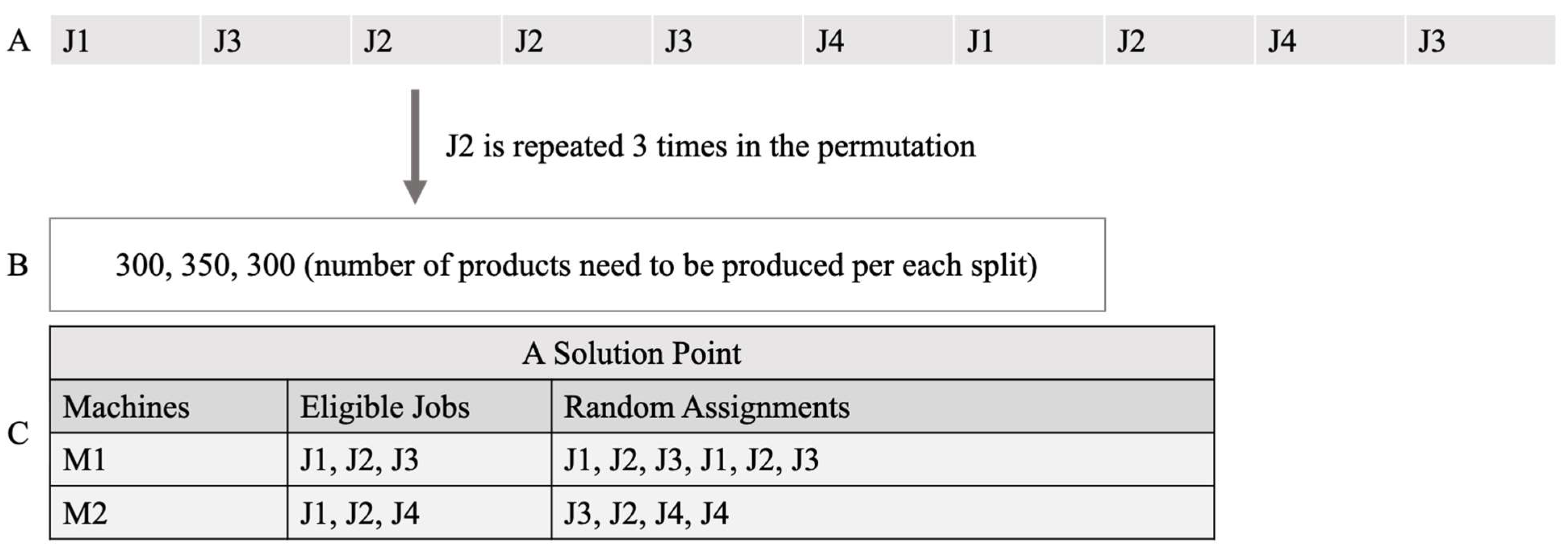
The first step of the GWO algorithm is the encoding representation scheme that shows a solution point in a structured way. For the real problem that we plan to study, the solution representation should reflect three main parts, including the sequence of jobs on every single machine, which is called a permutation, the number of products for each split ( in Table 2), and lists of jobs dedicated to each machine. The structure of each wolf is shown in Figure 1. Fundamentally, a solution point is constructed by a table similar to part C in Figure 1, with an associated number of products to each split (presented by B in Figure 1). A specific job necessitates the production of 950 units, with an engineering directive specifying a minimum production threshold of 300 units per segment. Consequently, this requirement breaks down into segmented quotas: 300 () + 350 () + 300 (), summing up to a total of 950 units. Due to limitations in renewable resources, the simultaneous production of these segments is not viable. However, it is worth noting that the order of on eligible machines remains flexible and feasible within these constraints. Please refer to the next section where the initial population generation is explained.
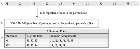
Figure 1.
Structure of wolf encoding. (A) Sequence of jobs’ splits, (B) products to be produced per each split, (C) Splits associated with each eligible machine.
4.2. Initial Population Generation
After encoding the structure of the wolf, the initial population of the grey wolf should be generated. As the GWO is a population-based metaheuristic algorithm, it needs to be produced with the size of search agents. Since the GWO algorithm is categorized among the stochastic metaheuristic algorithms, its initial population of the grey wolf will be generated randomly. Accordingly, we utilized this approach to produce the required numbers of the grey wolf for this study. Also, to avoid the unfeasibility of solution space, the heuristic algorithm is suggested for the proposed model of this study to avoid the unfeasible solution, which is shown in Algorithm 1.
| Algorithm 1: Randomly created feasible solutions. |
| Input Jobs, Economic Production, Machines, Machines Eligibility Based on economic production job, create splits Every split is equal to or greater than economic production. Every split contains the number of products that need to be produced. Assign the previous step to solution coding, 2nd segment “No. of Product per Split”. Create a random permutation of splits. Assign the previous step to solution coding, 1st segment “Permutation”. For each machine, create an empty list of assigned splits. For each split from each job, randomly assign it to a machine. While not an eligible machine is assigned, repeat the previous step. Assign this step to solution coding, 3rd segment “Split of Job Assigned to eligible Machine”. Evaluate the cost of solution coding. Assign this step to solution coding, 4th segment “Cost”. Output Create structured data containing all 4 segments |
The procedure of the proposed Algorithm 1 is explained as well. First, all jobs are split into smaller parts by having the knowledge about the minimum number of products in each split (presented by A and B in Figure 1). Then, a random sequence of all splits is generated (presented by A in Figure 1). Next, for splits belonging to each job, a list of the minimum number of products is mapped; therefore, each will have the number of products that need to be produced. After that, a list of eligible jobs is constructed for each machine, as shown in Figure 1C. Finally, the random assignment takes place by iteratively going through the random sequence and randomly assigning the split to an eligible machine (presented by C in Figure 1). However, please note that the same job cannot be operated by different machines simultaneously. In that case, one machine must finish operating the split, and then another machine can start operating the next split. Please consider “J2” presented by C in Figure 1.
4.3. Original Grey Wolf Optimizer
This section first aims to utilize the existing GWO algorithm and determine how it works. Second, we modify this algorithm based on the discrete nature of our problem to solve the model.
GWO works based on the social hierarchy of wolves. At the top level of the pyramid, the wolf exists, which belongs to the social hierarchy of Alpha. In the second level, the wolf with a group of betas stands, which helps the wolf with Alpha to make a better decision to attack the prey. Lastly, the last level of the pyramid is the wolf, located in the omega group. Also, the last group only eats and behaves normally like children or wolves with old age. To mathematically model the social hierarchy of grey wolves, the fittest solution will be considered as the Alpha. Also, the remaining solutions will be considered as Beta, Delta, and gamma; they will be utilized in the GWO algorithm.
Equations (18) and (19) provide the encircling prey formulation that was proposed by Mirjalili et al. [1], which are as follows:
where are coefficients vectors, and are positions of prey and grey wolves in the algorithm. Also are computed by Equations (20) and (21) as well.
Also, are random numbers that will be generated. Additionally, is a critical parameter of the GWO algorithm that will be decreased from 2 to 0 linearly using Equation (22).
In Equation (22), shows the counter of iterations in the main algorithm, while represents the total number of iterations that the problem needs to run. After that, the hunting will be started and guided by the Alpha. To mathematically formulate the hunting, we have the following:
where and are the approximate positions of Alpha, Beta, and gamma. Also, Equation (26) updates the positions of each wolf in the algorithm. Algorithm 2 shows the pseudocode of the GWO algorithm.
| Algorithm 2: The original GWO algorithm. |
| Input: Set the parameters of the GWO such as for I = 1 to number of search agents do Create a random solution. Calculate the value of the objective function (Minimization or Maximization) end for Set the best solution as Alpha. Set the second-best solution as Beta. Set the third-best solution as Delta. Initialize iteration it = 1 while it < MaxIteration do for it = 1 to number of search agents do Update the position of each grey wolf using Equation (26) end for Decrease the value of Alpha from 2 to 0 using Equation (22) Decrease A and C parameters. Calculate the value of the objective function of each grey wolf. Update , , and it = it + 1 end while Return the best wolf alpha |
4.4. Discrete Grey Wolf Optimizer
So far, we have understood how GWO works iteratively and efficiently. Therefore, this sub-section aims to modify the original version of the GWO algorithm to obtain a feasible solution for the proposed model of this study. Since GWO is proposed for the continuous optimization problem, some modifications need to be taken to solve the UPMSP.
To apply the mathematical formulation of the GWO algorithm proposed in Section 4.3, we applied the 2-opt algorithm proposed by Croes et al. [39], so that the UPMSP can be solved efficiently. The 2-opt algorithm belongs to the local search family, and it is widely used by many researchers to speed up convergence [40,41]. The 2-opt algorithm is first proposed for solving the popular travel salesman problem to find an optimal route along the existing routes of the network. Accordingly, we customized this algorithm based on our model to obtain the results.
The 2-opt algorithm, firstly, selects two jobs randomly from one permutation and, secondly, removes them from the current permutation and then reconnects all remaining jobs in the permutation together. These steps will be performed until all permutations in the algorithm are optimized. The purpose of this operation is to minimize the completion time of all jobs (Makespan), which is the objective function of this study.
Interestingly, we utilized the concept of hamming distance to alter the original GWO to a discrete GWO [40,41]. Also, some parameters of the GWO have been removed for the purpose of improving algorithm efficiency. Therefore, we modified Equations (23)–(25) to compute the new , and to reflect the discretion, which is as follows:
Equations (27)–(29) calculate the random number between 1 and hamming distance between wolves. Similarly, we proposed the 2-opt algorithm to update the positions of the wolves. Also, the wolf i executes number of the 2-opt algorithm in each iteration. Algorithm 3 shows the pseudocode of the discrete version of the GWO algorithm.
| Algorithm 3: The discrete GWO algorithm. |
| Input: Set the parameters of the GWO such as for i = 1 to number of search agents do Create a random solution. Calculate the value of the objective function (Minimization or Maximization) end for Set the best solution as Alpha. Set the second-best solution as Beta. Set the third-best solution as Delta. Initialize iteration it = 1 while it < MaxIteration do for it = 1 to number of search agents do Update the position of each grey wolf using Hamming Distance in Equations (27)–(29) end for Decrease the value of Alpha from 2 to 0 using Equation (22) Decrease A and C parameters. Calculate the value of the objective function of each grey wolf. Update , , and it = it + 1 end while Return the best wolf alpha |
5. Computational Experiments
This section provides the results of the UPMSP proposed in Section 3. First, we plan to solve the proposed model by considering different test problems in small and medium sizes and then solve a real case study of BIMC as discussed in this paper. Moreover, the proposed discrete GWO algorithm is coded on MATLAB R2021b software and runs on an Intel Core i5 CPU with 2.07 GHz speed and 8 GB of RAM.
5.1. Test Problem and Parameter Setting
To obtain the results, the model of this study is tested on a small size of the problem. Also, by doing so, we understand that our model works efficiently. The parameter value of the model and algorithm is provided in Table 3.

Table 3.
Parameter value of the model and algorithm.
5.2. Computational Results
After defining the parameters, the discrete GWO metaheuristic algorithm is implemented to obtain the results for each test problem in Table 4. The problem dimension is defined by the number of jobs, machines, parts of each job, renewable resources, and periods. The result and solution time of each problem has been provided and reported in Table 4.

Table 4.
Parameter value of the model and algorithm.
As can be seen from Table 4, by increasing the dimensions of the problem, the complexity of the model increases. This is due to the nature of the UPMSP proposed in Section 3. Also, we have seen that the CPLEX solver is not able to solve problem number 5 (10*5*2*2*4) or more due to the increase in the dimension of the problems. In this way, the discrete GWO is proposed to combat this issue by solving various problems in the fastest time.
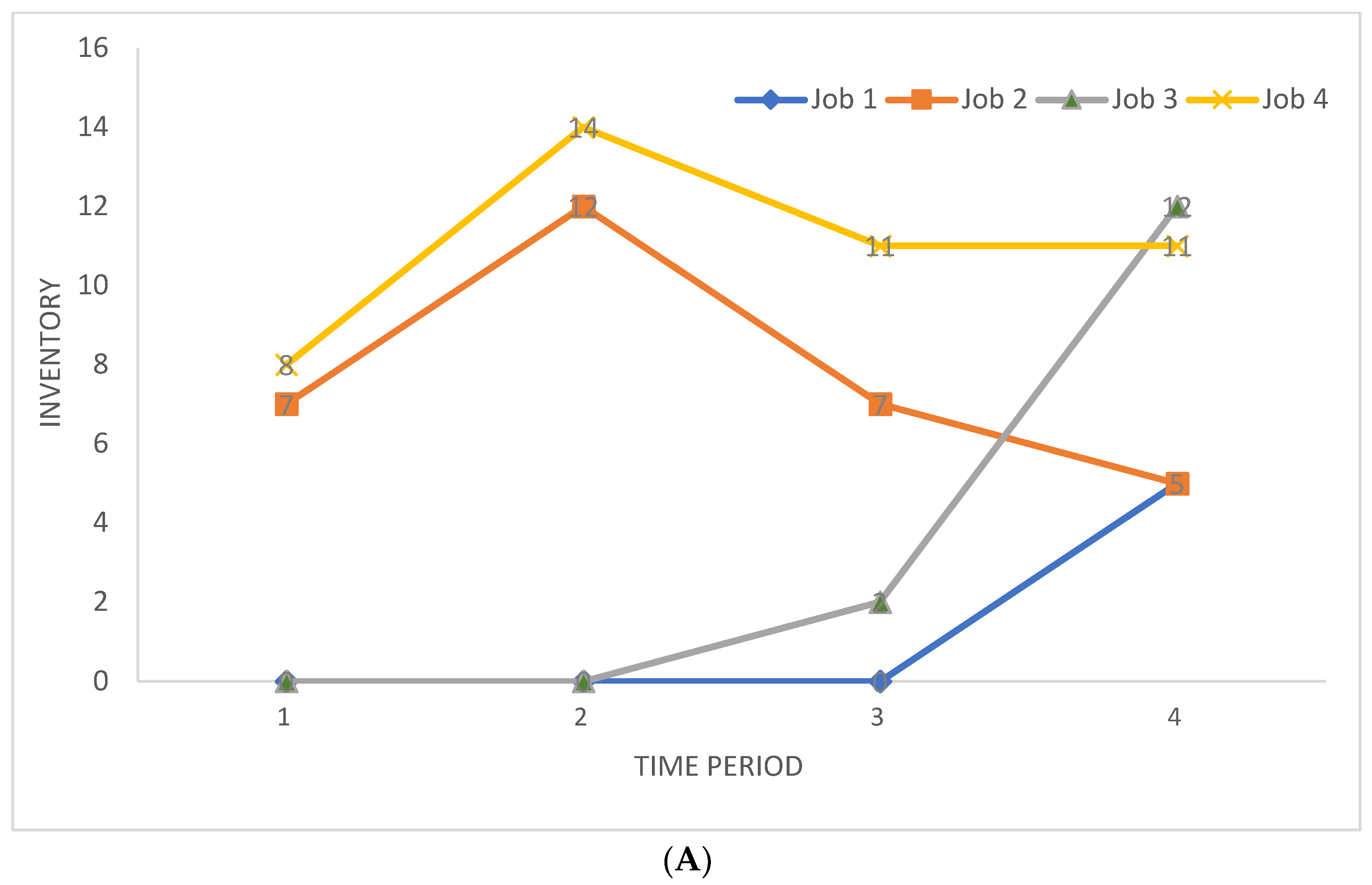
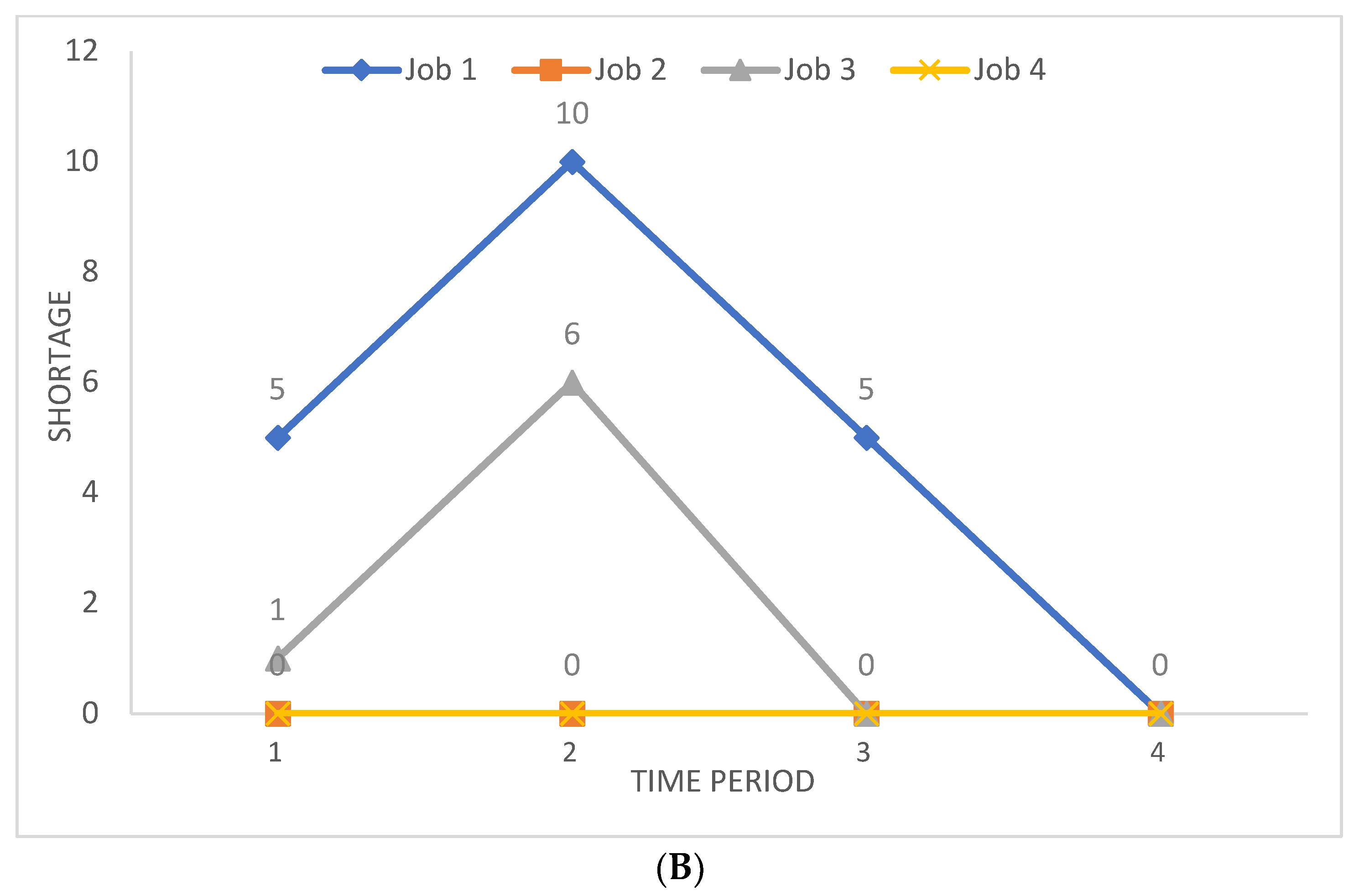
Interestingly, we provide the details of other variables defined in our model, including inventories and shortages, to avoid late fees. Because of the important role of these two variables, we provide the results of problem 1, where the number of jobs, machines, parts of each job, renewable resources, and periods are 4, 2, 2, 2, and 4 for these two variables. Figure 2 displays the results of two important inventory and shortage variables for problem 1 (4*2*2*2*4). The first thing that can be seen from Figure 2 is that when the inventory obtained a positive value, the shortage yielded zero. Also, the same thing can be interpreted and visible for the shortage variable. This is due to the nature of these two variables that we defined in this study. Also, the other thing that can be understood is that an increase in inventory value resulted in a decrease in shortage value, and the same thing for the shortage. This is due to the conflict that exists between these two variables in the inventory management problem.
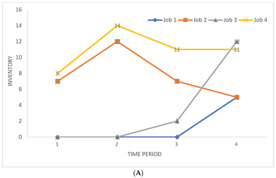
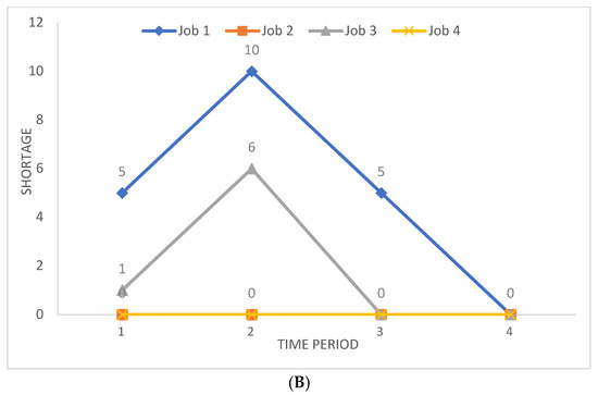
Figure 2.
Results of the inventory and shortage for the problem with a size of 4*2*2*2*4. (A) Inventory versus time, (B) Shortage versus time.
5.3. Results of a Case Study
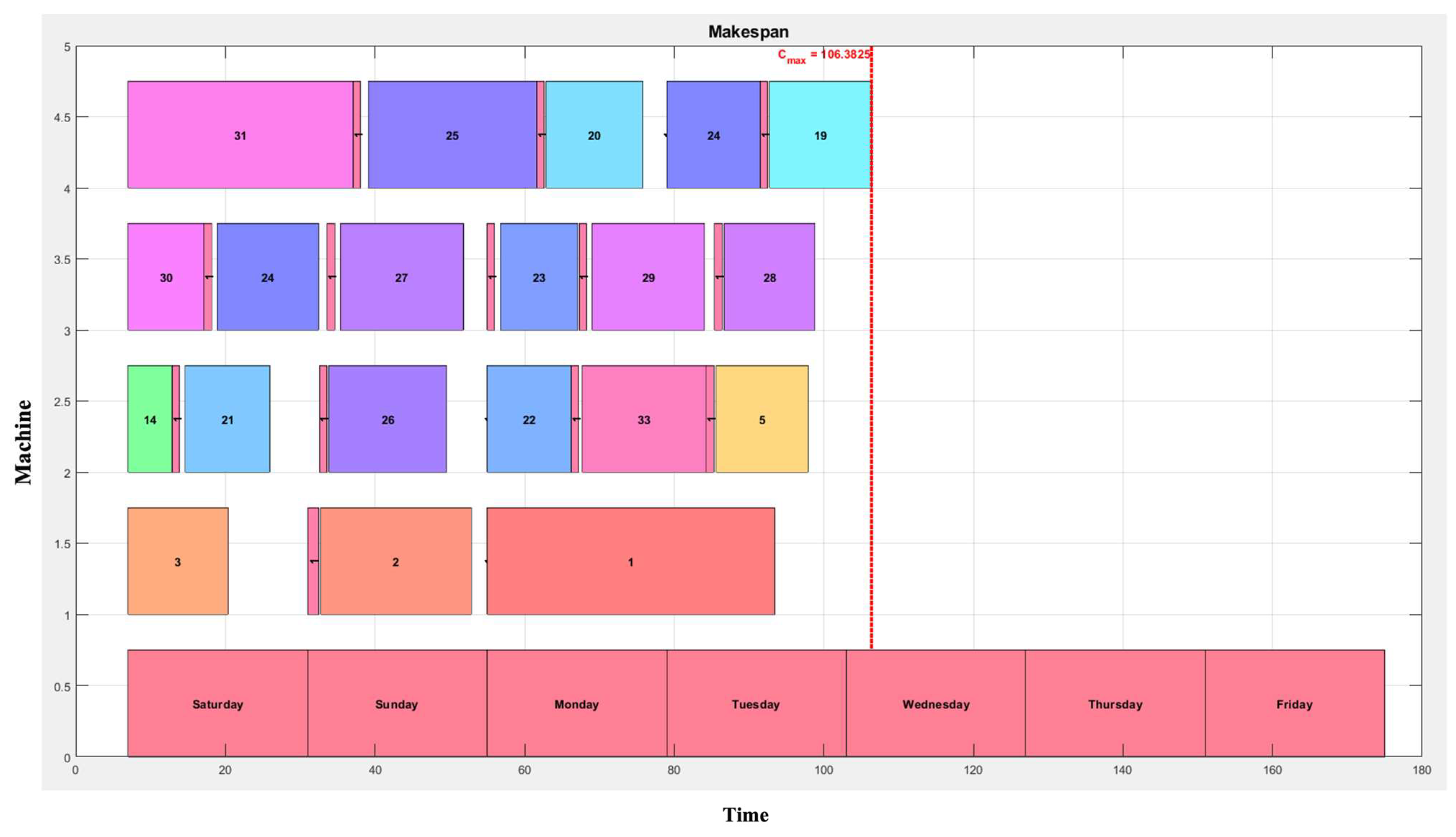
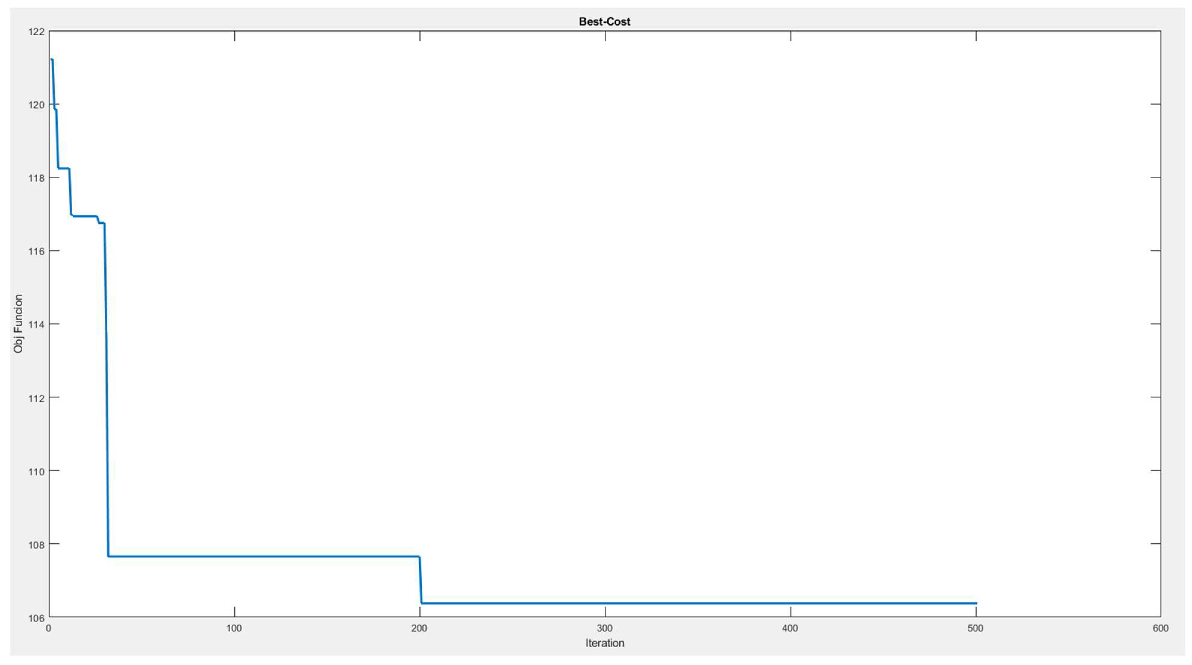
As stated earlier, this study considered the real case study of BIMC in Iran to address the UPAMSP by providing the results of the model in an efficient way. In this way, the real case study of BIMC includes 32 jobs that have been considered, which need to be produced on four machines seven days a week. The results of the UPMSP for the BIMC are shown in Figure 3. As can be seen in Figure 3, the optimal completion time of all 32 jobs over the four machines is 106.3825 h.

Figure 3.
Feasible solution of the real case study (optimal solution).
Also, the number of iterations, as shown in Figure 4, shows the convergence of the proposed discrete GWO in this study. As shown in Figure 4, the real case study has reached a stable condition after 200 iterations.
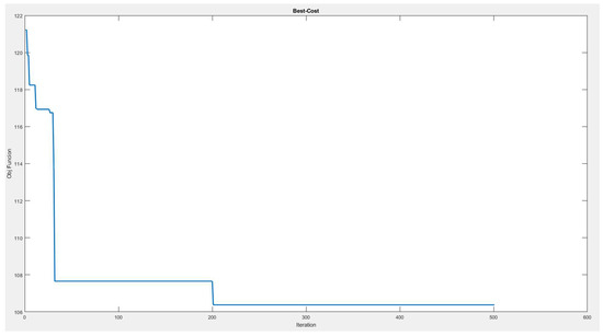
Figure 4.
Convergence curve for the real case study.
6. Conclusions
This paper studied a real case study of the UPMSP, which aimed at minimizing the completion time of all existing jobs over the machines within a period. Our proposed model integrated inventory with shortage along with splitting the jobs to complete the jobs in the shortest time. Due to the NP-hard nature of the UPMSP, we have utilized a metaheuristic approach named GWO, which was proposed by Mirjalili et al. [1] to find a near-optimal solution in a reasonable time. Also, because of the nature of GWO that has been proposed for continuous optimization problems, we modified the GWO to be compatible with the discrete problem. In this manner, we proposed a discrete GWO algorithm to fully solve the UPMSP in discrete space and search for feasible solutions. To validate the model of this study, we have tested the UPMSP on different problems with various sizes of jobs, machines, renewable resources, periods, and parts of each job and ran the model for the case study of this paper. Our results showed that increasing inventory led to a decrease in the shortage of various jobs in multiple time periods. Also, considering job splitting could help the planner obtain a lower completion time compared to the situation without job splitting.
Some suggestions have been provided for future studies. First, different objective functions can be investigated, including minimizing tardiness and lateness to be solved by the proposed discrete GWO algorithm. Second, the proposed UPMSP can be solved using other metaheuristic approaches. Lastly, various inventory policies accompanying varied types of perishable and non-perishable products can be included.
Author Contributions
M.A.: Methodology, solution algorithm, data collection, analysis, reviewing, and editing. M.M.: Methodology, solution algorithm, data collection, analysis, writing original draft, reviewing, and editing. T.J.P.: Data collection, reviewing, and editing. All authors have read and agreed to the published version of the manuscript.
Funding
This research received no external funding.
Institutional Review Board Statement
Not applicable.
Informed Consent Statement
Not applicable.
Data Availability Statement
The datasets used during the current study are available from the corresponding author upon reasonable request.
Conflicts of Interest
The authors declare that they have no competing interests.
References
- Afzalirad, M.; Rezaeian, J. Resource-constrained unrelated parallel machine scheduling problem with sequence dependent setup times, precedence constraints and machine eligibility restrictions. Comput. Ind. Eng. 2016, 98, 40–52. [Google Scholar] [CrossRef]
- Alharkan, I.; Saleh, M.; Ghaleb, M.A.; Kaid, H.; Farhan, A.; Almarfadi, A. Tabu search and particle swarm optimization algorithms for two identical parallel machines scheduling problem with a single server. J. King Saud Univ.-Eng. Sci. 2020, 32, 330–338. [Google Scholar] [CrossRef]
- Allahverdi, A. The third comprehensive survey on scheduling problems with setup times/costs. Eur. J. Oper. Res. 2015, 246, 345–378. [Google Scholar] [CrossRef]
- Arani, M.; Dastmard, M.; Momenitabar, M.; Liu, X. Unrelated Parallel Machine Scheduling Problem (UPMSP) Considering Work-in-Process and Finished Goods Inventories Subject to Resource Constraints and Due Dates: A Simulated Annealing. In Logistics and Supply Chain Management; Springer: Berlin/Heidelberg, Germany, 2020; Available online: https://link.springer.com/bookseries/7899 (accessed on 30 October 2021).
- Arık, O.A.; Schutten, M.; Topan, E. Weighted earliness/tardiness parallel machine scheduling problem with a common due date. Expert Syst. Appl. 2022, 187, 115916. [Google Scholar] [CrossRef]
- Asadpour, M.; Hodaei, Z.; Azami, M.; Kehtari, E.; Vesal, N. A green model for identical parallel machines scheduling problem considering tardy jobs and job splitting property. Sustain. Oper. Comput. 2022, 3, 149–155. [Google Scholar] [CrossRef]
- Bilge, Ü.; Kıraç, F.; Kurtulan, M.; Pekgün, P. A tabu search algorithm for parallel machine total tardiness problem. Comput. Oper. Res. 2004, 31, 397–414. [Google Scholar] [CrossRef]
- Chen, X.; Zhou, Y.; Tang, Z.; Luo, Q. A hybrid algorithm combining glowworm swarm optimization and complete 2-opt algorithm for spherical travelling salesman problems. Appl. Soft Comput. 2017, 58, 104–114. [Google Scholar] [CrossRef]
- Cheng, B.; Wang, Q.; Yang, S.; Hu, X. An improved ant colony optimization for scheduling identical parallel batching machines with arbitrary job sizes. Appl. Soft Comput. 2013, 13, 765–772. [Google Scholar] [CrossRef]
- Cheng, T.C.E.; Sin, C.C.S. A state-of-the-art review of parallel-machine scheduling research. Eur. J. Oper. Res. 1990, 47, 271–292. [Google Scholar] [CrossRef]
- Croes, G.A. A Method for Solving Traveling-Salesman Problems. Oper. Res. 1958, 6, 791–812. [Google Scholar] [CrossRef]
- de Souza, E.A.G.; Nagano, M.S.; Rolim, G.A. Dynamic Programming algorithms and their applications in machine scheduling: A review. Expert Syst. Appl. 2022, 190, 116180. [Google Scholar] [CrossRef]
- Fanjul-Peyro, L.; Perea, F.; Ruiz, R. Models and matheuristics for the unrelated parallel machine scheduling problem with additional resources. Eur. J. Oper. Res. 2017, 260, 482–493. [Google Scholar] [CrossRef]
- Fowler, J.W.; Mönch, L. A survey of scheduling with parallel batch (p-batch) processing. Eur. J. Oper. Res. 2022, 298, 1–24. [Google Scholar] [CrossRef]
- Gedik, R.; Kalathia, D.; Egilmez, G.; Kirac, E. A constraint programming approach for solving unrelated parallel machine scheduling problem. Comput. Ind. Eng. 2018, 121, 139–149. [Google Scholar] [CrossRef]
- Kaabi, J.; Harrath, Y. Scheduling on uniform parallel machines with periodic unavailability constraints. Int. J. Prod. Res. 2019, 57, 216–227. [Google Scholar] [CrossRef]
- Karagul, K.; Aydemir, E.; Tokat, S. Using 2-Opt based evolution strategy for travelling salesman problem. Int. J. Optim. Control Theor. Appl. (IJOCTA) 2016, 6, 103–113. [Google Scholar] [CrossRef]
- Karp, R.M. Reducibility among Combinatorial Problems. In Complexity of Computer Computations; Springer: New York, NY, USA, 1972; pp. 85–103. [Google Scholar] [CrossRef]
- Kim, Y.-D.; Shim, S.-O.; Kim, S.-B.; Choi, Y.-C.; Yoon, H.M. Parallel machine scheduling considering a job-splitting property. Int. J. Prod. Res. 2004, 42, 4531–4546. [Google Scholar] [CrossRef]
- Kim, J.-G.; Song, S.; Jeong, B. Minimising total tardiness for the identical parallel machine scheduling problem with splitting jobs and sequence-dependent setup times. Int. J. Prod. Res. 2020, 58, 1628–1643. [Google Scholar] [CrossRef]
- Koulamas, C.; Kyparisis, G.J. A modified LPT algorithm for the two uniform parallel machine makespan minimization problem. Eur. J. Oper. Res. 2009, 196, 61–68. [Google Scholar] [CrossRef]
- Kress, D.; Meiswinkel, S.; Pesch, E. Mechanism design for machine scheduling problems: Classification and literature overview. OR Spectr. 2018, 40, 583–611. [Google Scholar] [CrossRef]
- Lee, C.-H. A dispatching rule and a random iterated greedy metaheuristic for identical parallel machine scheduling to minimize total tardiness. Int. J. Prod. Res. 2018, 56, 2292–2308. [Google Scholar] [CrossRef]
- Lee, W.-C.; Chuang, M.-C.; Yeh, W.-C. Uniform parallel-machine scheduling to minimize Makespan with position-based learning curves. Comput. Ind. Eng. 2012, 63, 813–818. [Google Scholar] [CrossRef]
- Lee, W.-C.; Wu, C.-C.; Chen, P. A simulated annealing approach to makespan minimization on identical parallel machines. Int. J. Adv. Manuf. Technol. 2006, 31, 328–334. [Google Scholar] [CrossRef]
- Lei, D.; Yuan, Y.; Cai, J. An improved artificial bee colony for multi-objective distributed unrelated parallel machine scheduling. Int. J. Prod. Res. 2021, 59, 5259–5271. [Google Scholar] [CrossRef]
- Lin, Y.K.; Pfund, M.E.; Fowler, J.W. Heuristics for minimizing regular performance measures in unrelated parallel machine scheduling problems. Comput. Oper. Res. 2011, 38, 901–916. [Google Scholar] [CrossRef]
- Logendran, R.; Subur, F. Unrelated parallel machine scheduling with job splitting. IIE Trans. 2004, 36, 359–372. [Google Scholar] [CrossRef]
- Mirjalili, S.; Mirjalili, S.M.; Lewis, A. Grey Wolf Optimizer. Adv. Eng. Softw. 2014, 69, 46–61. [Google Scholar] [CrossRef]
- Nait Tahar, D.; Yalaoui, F.; Chu, C.; Amodeo, L. A linear programming approach for identical parallel machine scheduling with job splitting and sequence-dependent setup times. Int. J. Prod. Econ. 2006, 99, 63–73. [Google Scholar] [CrossRef]
- Park, T.; Lee, T.; Kim, C.O. Due-date scheduling on parallel machines with job splitting and sequence-dependent major/minor setup times. Int. J. Adv. Manuf. Technol. 2012, 59, 325–333. [Google Scholar] [CrossRef]
- Rudek, R. A fast neighborhood search scheme for identical parallel machine scheduling problems under general learning curves. Appl. Soft Comput. 2021, 113, 108023. [Google Scholar] [CrossRef]
- Sarıçiçek, İ.; Çelik, C. Two meta-heuristics for parallel machine scheduling with job splitting to minimize total tardiness. Appl. Math. Model. 2011, 35, 4117–4126. [Google Scholar] [CrossRef]
- Wang, X.; Cheng, T.C.E. A heuristic for scheduling jobs on two identical parallel machines with a machine availability constraint. Int. J. Prod. Econ. 2015, 161, 74–82. [Google Scholar] [CrossRef]
- Yang, D.-L.; Yang, S.-J. Unrelated parallel-machine scheduling problems with multiple rate-modifying activities. Inf. Sci. 2013, 235, 280–286. [Google Scholar] [CrossRef]
- Yeh, W.-C.; Chuang, M.-C.; Lee, W.-C. Uniform parallel machine scheduling with resource consumption constraint. Appl. Math. Model. 2015, 39, 2131–2138. [Google Scholar] [CrossRef]
- Yepes-Borrero, J.C.; Villa, F.; Perea, F.; Caballero-Villalobos, J.P. GRASP algorithm for the unrelated parallel machine scheduling problem with setup times and additional resources. Expert Syst. Appl. 2020, 141, 112959. [Google Scholar] [CrossRef]
- Yunusoglu, P.; Topaloglu Yildiz, S. Constraint programming approach for multi-resource-constrained unrelated parallel machine scheduling problem with sequence-dependent setup times. Int. J. Prod. Res. 2022, 60, 2212–2229. [Google Scholar] [CrossRef]
- Zeng, Y.; Che, A.; Wu, X. Bi-objective scheduling on uniform parallel machines considering electricity cost. Eng. Optim. 2018, 50, 19–36. [Google Scholar] [CrossRef]
- Zhang, L.; Deng, Q.; Gong, G.; Han, W. A new unrelated parallel machine scheduling problem with tool changes to minimise the total energy consumption. Int. J. Prod. Res. 2020, 58, 6826–6845. [Google Scholar] [CrossRef]
- Zhang, L.; Deng, Q.; Lin, R.; Gong, G.; Han, W. A combinatorial evolutionary algorithm for unrelated parallel machine scheduling problem with sequence and machine-dependent setup times, limited worker resources and learning effect. Expert Syst. Appl. 2021, 175, 114843. [Google Scholar] [CrossRef]
Disclaimer/Publisher’s Note: The statements, opinions and data contained in all publications are solely those of the individual author(s) and contributor(s) and not of MDPI and/or the editor(s). MDPI and/or the editor(s) disclaim responsibility for any injury to people or property resulting from any ideas, methods, instructions or products referred to in the content. |
© 2024 by the authors. Licensee MDPI, Basel, Switzerland. This article is an open access article distributed under the terms and conditions of the Creative Commons Attribution (CC BY) license (https://creativecommons.org/licenses/by/4.0/).

