Article

Forecasting the Natural Gas Supply and Consumption in China Using a Novel Grey Wavelet Support Vector Regressor

1
School of Mathematics and Physics, Southwest University of Science and Technology, Mianyang 621010, China
2
Center for Information Management and Service Studies of Sichuan, Southwest University of Science and Technology, Mianyang 621010, China
3
School of Management Science and Real Estate, Chongqing University, Chongqing 400045, China
*
Author to whom correspondence should be addressed.
Systems 2023, 11(8), 428; https://doi.org/10.3390/systems11080428
Submission received: 30 June 2023 / Revised: 25 July 2023 / Accepted: 11 August 2023 / Published: 15 August 2023

Abstract

:
Natural gas is playing an important role in the reconstruction of the energy system of China. Natural gas supply and consumption indicators forecasting is an important decision-making support for the government and energy companies, which has attracted considerable interest from researchers in recent years. In order to deal with the more complex features of the natural gas datasets in China, a Grey Wavelet Support Vector Regressor is proposed in this work. This model integrates the primary framework of the grey system model with the kernel representation employed in the support vector regression model. Through a series of mathematical transformations, the parameter optimization problem can be solved using the sequential minimal optimization algorithm. The Grey Wolf Optimizer is used to optimize its hyperparameters with the nested cross-validation scheme, and a complete computational algorithm is built. The case studies are conducted with real-world datasets from 2003–2020 in China using the proposed model and 15 other models. The results show that the proposed model presents a significantly higher performance in out-of-sample forecasting than all the other models, indicating the high potential of the proposed model in forecasting the natural gas supply and consumption in China.

1. Introduction

Energy forecasting is of great significance for understanding and anticipating the future dynamics of the global energy landscape. As a versatile and abundant primary energy, natural gas plays a vital role in meeting the energy demands of various sectors, including power generation, heating, industrial processes, and transportation. Accurate forecasting of natural gas is crucial for policymakers to develop effective energy strategies and make informed decisions about energy infrastructure, environmental regulations, and energy security. However, as countries strive to reduce their reliance on fossil fuels and transition towards cleaner energy alternatives, the demand for natural gas may undergo fluctuations. Additionally, geopolitical factors, such as regional conflicts or trade agreements, can influence natural gas consumption patterns by affecting supply routes and prices. In a word, the time series of natural gas is influenced by multiple factors and exhibits typical complex and irregular characteristics. Traditional forecasting models face challenges in accurately forecasting such patterns. The popular energy forecasting methods include statistical (or empirical) models, machine learning models, and grey system models at present.
The time series models are one of the most used statistical models, which consist of the autoregressive integrated moving average (ARIMA) model, the autoregressive moving average (ARMA) model, and the seasonal autoregressive integrated moving average model [1]. However, the linear structure of time series models often makes them fail to forecast the nonlinear time series accurately. Machine learning models have unique advantages in handling nonlinear time series. Machine learning models mainly include neural network models [2,3,4], models based on kernel [5,6], and ensemble models [7]. Although machine learning models excel in handling nonlinear system problems, they require a significant amount of training data and impose certain hardware requirements. Furthermore, machine learning models possess intricate nonlinear parameters, which may lead to overfitting. Given the limitations of the aforementioned approaches, grey system models have gained wide applicability due to their ability to model with limited data and accommodate both linear and nonlinear problems.
Since Professor Deng [8] proposed the grey system theory, many researchers have made contributions to the development of the grey system in different fields. Examples include nuclear energy consumption [9,10,11,12], wind energy [13,14], electricity consumption [15,16], and oil production [17,18]. Currently, mainstream grey models can be broadly categorized into linear models and nonlinear models. The GM(1,1) model is the most classical linear grey model, while it has inherent issues in modeling mechanisms. Therefore, many scholars have proposed other linear grey models based on the GM(1,1) model. For example, Chen et al. [19] improved the background value of the grey model using Gaussian–Legendre integration. Xie et al. [20] first proposed the idea of grey discrete modeling and established the discrete grey model. Xu et al. [21] firstly demonstrated that grey inputs can vary with time and possess dynamic variability. Then, Cui et al. [22] employed a linear function of time as the grey input instead of the original constant grey input. However, the forecasting of natural gas is a complex nonlinear problem, and linear grey models have significant limitations when facing such a problem.
Nonlinear grey models can better capture the nonlinear relationships in raw data. In recent years, an increasing number of studies have focused on nonlinear grey system models. For instance, Zhou et al. [23] proposed a novel discrete grey model considering nonlinearity and fluctuations. Chen et al. [24] proposed the fractional Hausdorff derivative grey model based on fractional order calculation. Qian et al. [25] proposed a grey model with time power and demonstrated its feasibility. Zeng et al. [26] presented a grey model that incorporates lagged dependent variables, linear correction terms, and stochastic disturbance terms. Liu et al. [27] proposed a grey neural network and input–output combined forecasting model for forecasting the primary energy consumption in Spanish economic sectors. Ma et al. [28] proposed a novel wavelet kernel-based grey system model by combining the grey system modeling and wavelet kernel-based machine learning and applied it to the urban natural gas consumption forecasting in Kunming, China, which takes advantage of the nonlinearity and periodicity ability of the wavelet kernel. However, existing nonlinear grey system models are often constructed using specific functions, resulting in relatively fixed structures of these models, making them less adaptable to handle more general nonlinear characteristics.
The hyperparameters optimization of nonlinear grey models has also emerged as a popular research topic in recent years. Intelligent optimization algorithms are a class of algorithms based on heuristic search strategies, which are capable of finding solutions that are close to the global optimum within a limited number of iterations. This characteristic makes them particularly effective in handling highly nonlinear, multimodal, and complex optimization problems, leading to their widespread application in recent years. At present, the most popular algorithms are Grey Wolf Optimization (GWO) [29], Particle Swarm Optimization (PSO) [30], and the Genetic Algorithm (GA) [31]. For instance, Cai et al. [32] introduced GWO for tuning the hyperparameters of long short-term memory networks. Heydari et al. [33] employed GWO to optimize the Generalized Regression Neural Network. Sebayang et al. [34] used GWO to tune the hyperparameters of an Artificial Neural Network. Barman et al. [35] compared the performance of GWO, PSO, and GA, showing that GWO outperformed other algorithms.
In summary, nonlinear grey models can better fit complex data patterns, effectively handle outliers and noisy data, and improve the accuracy of predictions. In previous work, researchers employed specific functions as the grey input to construct nonlinear grey models. In order to address the broader spectrum of nonlinear characteristics, the kernel trick based on the support vector regression with wavelet kernel is employed to build a novel Grey Wavelet Support Vector Regressor. The  ε -insensitive loss function is used to build the optimization problem for training the model, which is transformed to a convex quadratic programming and then solved by the sequential minimal optimization algorithm. The GWO is incorporated to optimize the hyperparameters of the suggested model, thereby finalizing the training and forecasting process of the model.
The subsequent sections of this paper are organized as follows: Section 2 presents the proposed Grey Wavelet Support Vector Regressor, including all the modeling procedures and algorithms; Section 3 presents the hyperparameter optimization by the grey wolf optimizer; Section 4 demonstrates the case studies conducted to forecast China’s total natural gas supply (available for consumption) and total natural gas consumption using the proposed model. A comparison with other grey system models is provided, and the findings are summarized in Section 5.

2. The Proposed Grey Wavelet Support Vector Regressor

In this section, the proposed Grey Wavelet Support Vector Regressor (GWSVR) is presented, which uses the main formulation of grey system models and the loss function of the support vector regression.

2.1. Grey System Model with Nonlinear Mapping and Its Solution

A general formulation of the grey system model with nonlinear effect by time can be represented by:
d y ( 1 ) ( t ) d t + b y ( 1 ) ( t ) = g ( t ) ,
where g ( t ) is a nonlinear function of time t, and  y ( 1 ) ( t ) = τ = 1 t y ( 0 ) ( τ ) is the first order accumulation, which is often abbreviated as 1-AGO. In previous work, researchers used some specific functions such as a linear function and an exponential function to build specific grey system models. In order to deal with more general nonlinear features, a nonlinear mapping is used in this work, which is defined as follows:
ϕ : R F ,
where R is the 1-D set of real numbers, and F is the feature space, which is generally high-dimensional linear space. Within this nonlinear mapping, the nonlinear function can be linearly expressed in the feature space as
g ( t ) = ω T ϕ ( t ) + u ,
where the vector ω F is the weight, and u is a bias. Then, (1) of the grey system model can be re-written as
d y ( 1 ) ( t ) d t + b y ( 1 ) ( t ) = ω T ϕ ( t ) + u .
The whitening Equation (4) is a typical ordinary differential equation, of which the general solution is
y ( 1 ) ( t ) = y ( 0 ) ( 1 ) e b ( t 1 ) + 1 t e b ( t τ ) · ω T ϕ ( τ ) + u d τ .

2.2. The ε -Insensitive Loss for the Proposed Model

In order to estimate the parameters and the nonlinear function of the grey system model presented above, we need to first derive its discrete formulation. In previous work, a general way has been to integrate the whitening Equation (4) in a small interval (e.g., [ k 1 , k ] ). In this work, we make a tiny variation, which averages the time t of the nonlinear mapping instead of averaging the nonlinear function to make the model simpler without loss of effectiveness. The discrete formulation can be written as
y ( 0 ) ( k ) + b s ( 1 ) ( k ) = ω T ϕ ( k 1 2 ) + u ,
where s ( 1 ) ( k ) = 1 2 y ( 1 ) ( k ) + y ( 1 ) ( k 1 ) , k = 2 , , n are called the background values.
Then, the ε -insensitive loss used in this work can be given by
min a , ω 1 2 b 2 + ω 2 + C i = 1 N ς i + ς i s . t . y ( 0 ) ( k ) + b s ( 1 ) ( k ) ω T ϕ ( k 1 2 ) u ε + ς i ω T ϕ ( k 1 2 ) b s ( 1 ) ( k ) + u y ( 0 ) ( k ) ε + ς i ς i , ς i 0 .
The term C is often called the regularization parameter, which controls the fitting error and scale of the parameters b and ω . The  ε is a threshold, which limits the fitting errors of the model, and the ς i , ς i are the slack variables that make the regularization problem more feasible. This formulation is different to the commonly used least squares method, which not only minimizes the training errors of the model but also reduces the scale of the parameters b and ω , and this way, the model has higher generality in the real-world cases.
However, the Formulation (7) is not computable at present, as the nonlinear mapping is still unknown. To make it easier to solve, an extended nonlinear mapping is introduced as
φ : R × R R × F ,
which maps the vector s ( 1 ) ( k ) , k 1 2 T to s ( 1 ) ( k ) , ϕ ( k 1 2 ) T . Let the weighted vector be ω = b , ω T , we have
b s ( 1 ) ( k ) + ω T ϕ ( k 1 2 ) = ω T φ ( k ) ,
and then we can re-write Equation (7) as
min a , ω 1 2 ω 2 + C i = 1 N ς i + ς i s . t . y ( 0 ) ( i ) ω T φ ( i ) u ε + ς i ω T φ ( k ) + u y ( 0 ) ( i ) ε + ς i ς i , ς i 0 .
And now Equation (10) is essentially equivalent to the primal problem of the support vector regression introduced in [36]. Within this formulation, the corresponding Lagrangian function can be constructed as
L : = 1 2 ω 2 + C i = 2 n ς i + ς i i = 2 n η i ς i + η i ς i i = 2 n ι i ε + ς i y ( 0 ) ( i ) + ω T φ ( i ) + u i = 2 n ι i ε + ς i ω T φ ( i ) u + y ( 0 ) ( i ) ,
where ι i , ι i ( i = 2 , , n ) are the Lagrangian multipliers, which are nonnegative and satisfy ι i · ι i 0 . By setting the partial derivatives L b , L ω , L ς ( ) to be zeros, we can obtain some very important equalities as:
i = 2 n ι i ι i = 0 ω = i = 2 n ι i ι i φ ( i ) ι i ( ) = C η i ( ) .
According to Mercer’s condition, a Mercer kernel can be used as the inner product of the feature space, i.e., K ( , k ) = ϕ T ( ) ϕ ( k ) . Within this theorem, we can deduce the following equality
ω T φ ( k ) = i = 2 n ι i ι i φ T ( i ) φ ( k ) = i = 2 n ι i ι i s ( 1 ) ( i ) , ϕ T ( i 1 2 ) s ( 1 ) ( k ) ϕ ( k 1 2 ) = i = 2 n ι i ι i s ( 1 ) ( i ) s ( 1 ) ( k ) + ϕ T ( i 1 2 ) ϕ ( k 1 2 ) = i = 2 n ι i ι i s ( 1 ) ( i ) s ( 1 ) ( k ) + K ( i 1 2 , k 1 2 ) .
By substituting the equalities in (12) and (13) within a Mercer’s kernel, we obtain the dual formulation of the primal (10) as
max ι , ι 1 2 i , j = 2 n ι i ι i ι j ι j s ( 1 ) ( i ) s ( 1 ) ( j ) + K ( i 1 2 , j 1 2 ) ε i = 2 n ι i + ι i + i = 2 n y ( 0 ) ( i ) ι i ι i s . t . i = 2 n ι i ι i = 0 and ι i , ι i [ 0 , C ] .
It can be seen that the dual formulation is only involved in the computation of the Lagrangian multipliers, and it is now computationally feasible to solve.

2.3. The Kernel Representation and the Wavelet Kernel

Within the above results, the nonlinear function can now be explicitly written as
g ( t ) = ω T ϕ ( t ) + u = i = 2 n ι i ι i K ( i 1 2 , t ) + u .
The wavelet kernel function is used to represent the nonlinear function, which is defined as
K ( , k ) = exp k 2 2 ν 2 · cos 1.75 ( k ) ν ,
where ν is the kernel parameter, which governs the degree of nonlinearity and periodicity exhibited by the wavelet kernel. The cosine term of the wavelet kernel function reflects the degree of periodicity of the samples, and the exponential part reflects the nonlinearity of the samples. It is very interesting to see that the exponential part is mathematically equivalent to the Gaussian kernel, which has high performance in dealing with nonlinearities. Considering the structure of the wavelet kernel, it is often more flexible to deal with different spectrums of the datasets, which can be expected to make the forecasting model perform better in nonlinear time series.

2.4. Training Algorithm for the GWSVR

In order to make the model computationally feasible, we should solve the dual problem (14) to obtain the optimal values of the Lagrangian multipliers ι , ι . It can be seen that this formulation is mathematically equivalent to the dual problem of the standard support vector regression model introduced in [36]; thus, it can also be solved by the sequential minimal optimization (SMO) algorithm, of which the key points are presented in this subsection.
For convenience, the following notation is used
q i , j = s ( 1 ) ( i ) s ( 1 ) ( j ) + K ( i 1 2 , j 1 2 ) .
The main idea of the SMO is to minimize the objective function in a “pair-by-pair” way, which minimizes only two variables during each iteration. For the regression problem, two subscripts are selected, and the corresponding variables are optimized at this iteration. Noticing that the multipliers with same subscripts cannot be nonnegative at the same time, only two variables with different subscripts are updated during each iteration.
Let the selected two subscripts be 1 , 2 , and the subproblem of the dual problem (14) can be written as
max ι 1 ( ) , ι 2 ( ) 1 2 ι 1 ι 1 2 q 1 , 1 + ι 2 ι 2 2 q 2 , 2 + 2 ι 1 ι 1 ι 2 ι 2 q 1 , 2 ε ι 1 + ι 1 + ι 2 + ι 2 + y ( 0 ) ( 1 ) ι 1 ι 1 + y ( 0 ) ( 1 ) ι 1 ι 1 + r ( ι ) ,
where ι is the vector of other multipliers, and r ( ι ) is the sum of the rest of the terms, which are independent of the variables ι 1 ( ) , ι 2 ( ) , and it is regarded as constant during each iteration.
Noticing that the multipliers should satisfy the first equation in (12), the subproblem is essentially a constrained programming. The SMO updates the two variables in the following way
ι 1 ( ) = ι 1 ( ) t , ι 2 ( ) = ι 2 ( ) + t .
Within this updating rule, the multipliers can always satisfy the constraints during the iterations. By substituting (19) into the subproblem (18), the objective function is only with respect to t, and the subproblem turns to be a univariate optimization problem, which can be solved analytically.
The bias u can be computed when the optimal multipliers are obtained, which can be approximated by the average value of the partial derivatives of the objective function in (14) with respect to every multiplier.
By comparing Equations (13) and (9), it is easy to obtain the explicit estimation of the parameter b, which can be written as
b = i = 2 n ι i ι i s ( 1 ) ( i ) .
Above all, all the parameters can be obtained by using the SMO algorithm and the formulae presented above. The implementation of the SMO is based on the work of Lin et al. [37], which is one of the most stable versions at present.

2.5. Response Function and the Predicted Values

In order to make predictions, the continuous formulation of the general solution of the whitening Equation (4) should be discretized. In this work, we average the time point to reach an approximation of the convolutional integral of the solution (5); then, its discrete formulation can be obtained as
y ^ ( 1 ) ( k ) = y ( 0 ) ( 1 ) e b ( k 1 ) + τ = 2 k e b ( k τ + 1 2 ) g ( τ 1 2 ) = y ( 0 ) ( 1 ) e b ( k 1 ) + τ = 2 k e b ( k τ + 1 2 ) i = 2 n ι i ι i K ( i 1 2 , τ 1 2 ) + u .
This formulation is different to the previous work but is much easier to implement. Then, the predicted values can be obtained by first order differencing as
y ^ ( 0 ) ( k ) = y ^ ( 1 ) ( k ) y ^ ( 1 ) ( k 1 ) , k = 2 , 3 , , n ,
and y ^ ( 0 ) ( 1 ) = y ( 0 ) ( 1 ) .

2.6. The Complete Overal Computational Algorithm

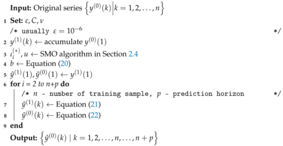
For application’s sake, a complete algorithm of the proposed GWSVR (Algorithm 1) is presented in this subsection as a piece of pseudo code.   
Algorithm 1: Overall computation algorithm of GWSVR
Systems 11 00428 i001
Within the above computational steps, one can obtain the values predicted by the GWSVR model from the initial point to the n + p point.

3. Hyperparameter Optimization by the Grey Wolf Optimizer

Within the high performance of the kernel representation, the model can be easily trapped in the overfitting status. Hence, selecting the appropriate hyperparameters is crucial to enhance the model’s performance when applied to out-of-sample datasets.

3.1. Construction of the Hyperparameter Optimization Scheme

In this study, the hold-out scheme is employed, which can be regarded as a modified version of nested cross validation specifically designed for time series forecasting models. The criterion used for model selection is to minimize the mean absolute percentage error (MAPE) on the validation set. The model is trained using the preceding series to evaluate its performance on the validation set. The objective function is constructed based on the aforementioned considerations as
min C , ν 1 n valid i = n train + 1 n train + n valid y ^ ( 0 ) ( i ) y ( 0 ) ( i ) y ( 0 ) ( i ) × 100 % .
The corresponding constraints can be presented as follows:
y ^ ( 0 ) ( 1 ) = y ( 0 ) ( 1 ) ι i ( ) , b , u   obtained   by   Algorithm   1 y ^ ( 1 ) ( k ) = y ( 0 ) ( 1 ) e b ( k 1 ) + τ = 2 k e b ( k τ + 1 2 ) i = 2 n ι i ι i K ( i 1 2 , τ 1 2 ) + u y ^ ( 0 ) ( k ) = y ^ ( 1 ) ( k ) y ^ ( 1 ) ( k 1 ) , k = 2 , 3 , , n .
The optimization problem for selecting the hyperparameters is essentially a nonlinear programming with equality constraints, which can not be solved by traditional numerical optimization algorithms. Thus, an intelligent optimizer is used in this work.

3.2. The Grey Wolf Optimizer

The Grey Wolf Optimizer (GWO) is a metaheuristic algorithm introduced by Mirjalili et al. in 2014, inspired by the hunting behavior of grey wolves in nature [29]. This optimization method has gained significant attention due to its efficient handling of complex optimization problems. The GWO algorithm employs mathematical formulas to emulate the social hierarchy and hunting strategies of grey wolves.
The grey wolf optimizer categorizes the wolves into four levels: ι , β , δ , and  ω . These designations represent the wolves’ fitness levels, ranked in descending order. The  ι wolf denotes the best solution, while the ω wolf represents the poorest solution. The primary operation of the GWO algorithm involves updating the positions of the wolves, also referred to as agents, based on the current positions of the ι , β , and  δ wolves. Initially, the distance D between the wolves is mathematically defined as follows:
D = 2 · r 2 · X p ( t ) X ( t ) ,
where X represents the position of a grey wolf, t indicates the current iteration, and  X p denotes the vector of the prey’s position.
Then, the position-updating behavior is defined as
X ( t + 1 ) = X p 2 a · r 1 a · D ,
where r 1 , r 2 are random vectors in 0 , 1 , and the components of a are linearly decreased from 2 to 0 at each process of iteration.
Based on the social hierarchy and encircling prey processes, the hunting process of the GWO algorithm employs four primary equations to update the positions of the wolves iteratively based on Equation (25). By taking the mean value of each update, the best position X ( t + 1 ) is represented as:
X ( t + 1 ) = X 1 + X 2 + X 3 3 .
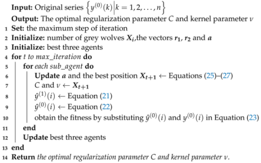
The integral computational algorithm for hyperparameter tuning based on the GWO algorithm is outlined in Algorithm 2.   
Algorithm 2: Algorithm for solving the optimization problem by GWO
Systems 11 00428 i002

4. Applications

4.1. Data Collection and Preprocessing

For this study, annual data on the Total Natural Gas Available for Consumption (measured in 100 million cubic meters, abbreviated as 100 million cu.m) and the Total Natural Gas Consumption (100 million cu.m) were collected from the National Bureau of Statistics of China (NBS) (https://data.stats.gov.cn/english/easyquery.htm?cn=C01 (accessed on 27 June 2023)). The data spans from 2003 to 2020, with the years 2003 to 2014 designated as the in-sample set. Among the in-sample data, the years 2003 to 2012 were used for model fitting, while the years 2013 to 2014 served as a validation set for hyperparameter tuning. The data from 2015 to 2020 remained reserved exclusively as the testing dataset, allowing for the evaluation of the model’s predictive capabilities on unseen data. This approach provides a reliable measure of the model’s performance in real-world scenarios. In addition, the data were subjected to normalization using MinMax scaling before conducting the experiments, which transformed the data into an interval 0 , 1 , facilitating fair comparisons and preventing any undue influence from variables with different scales or units. Another process is that the time t in the proposed model was accumulated in order to make the feature smoother.

4.2. Benchmarked Models for Comparisons and Evaluation Metrics

To assess the performance of the proposed grey wavelet support vector regressor (GWSVR) model, fifteen regular benchmark grey system models were utilized for model performance comparison, along with ten evaluation metrics. These benchmark models included the conventional grey model (GM) [8], nonhomogeneous grey model (NGM) [22], discrete grey model (DGM) [38], nonhomogenous discrete grey forecasting model (NDGM) [38], nonhomogeneous grey Bernoulli model (NGBM) [39], fractional-order grey model (FGM) [40], fractional-order nonhomogeneous grey model (FNGM) [41], fractional-order discrete grey model (FDGM) [42], fractional-order nonhomogeneous discrete grey model (FNDGM) [43], new information priority grey model (NIPGM) [44], new information priority nonhomogeneous grey model (NIPNGM) [45], new information priority discrete grey model (NIPDGM) [46], new information priority nonhomogeneous discrete grey model (NIPNDGM) [47], nonlinear grey Bernoulli model with fractional order accumulation (FNGBM) [48], and the new information priority nonlinear grey Bernoulli model (NIPNGBM). For fair comparisons, the benchmark models with hyperparameters were also optimized based on the GWO algorithm. In addition, a comprehensive set of evaluation metrics (as shown in Table 1) was employed to quantitatively measure and analyze various aspects of the model performance.

4.3. Forecasting Results and Analysis

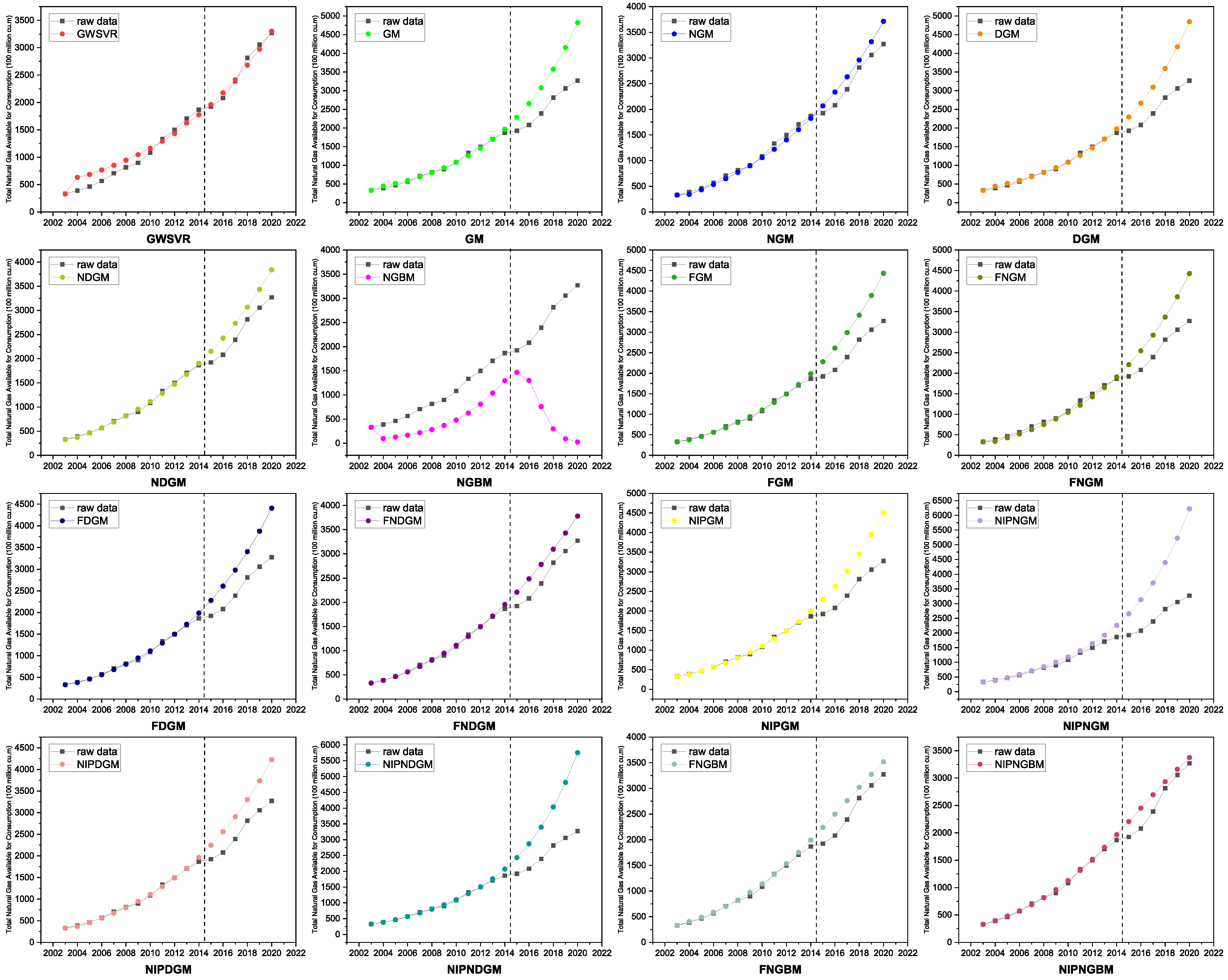
4.3.1. Case I: Forecast of the Total Natural Gas Available for Consumption in China

Figure 1 displays all the predicted values for the forecast of the total natural gas available for consumption. Additionally, the selected optimal hyperparameters and training time of all models are listed in Table 2, and Table 3 presents the evaluation metrics for the out-of-sample analysis. Notably, the GWSVR model demonstrates superior performance in out-of-sample forecasting, as evidenced by Figure 1. Conversely, the linear grey system models (GM and DGM) exhibit poor forecasting accuracy, with predicted values deviating significantly from the actual data. This discrepancy can be attributed to overfitting issues within these models. Additionally, the NGBM fails to capture the correct trend and exhibits an inaccurate predictive decay tendency. Furthermore, the other grey system models display a common limitation of poor out-of-sample prediction performance compared to their in-sample prediction performance, particularly struggling to accurately predict values near inflection points. In contrast, the GWSVR model effectively captures these inflection points, as evidenced by the close alignment of its predicted values with the original data.
Upon examining the out-of-sample performance evaluation metrics depicted in Table 3, it becomes apparent that the GWSVR model consistently surpasses other benchmarked grey system models. The MAPE values achieved by the GWSVR model range from 6.645278% to 66.479172%, indicating its superior performance across the evaluated scenarios. Notably, the R 2 values for the other grey system models are relatively small, with the NGBM model exhibiting a particularly low R 2 value of −18.7624. Additionally, none of the other grey system models achieve an R 2 value exceeding 0.9. Conversely, the GWSVR model achieves an R 2 value of 0.974704, providing compelling evidence of its proficiency in out-of-sample forecasting tasks. The comprehensive out-of-sample forecasting results of all the models are presented in Table 4; it is interesting to see that the maximum error of the GWSVR model is still less than the minimum error of the benchmarked models except for the NIPNGBM model, demonstrating the superior capability of the GWSVR model. Furthermore, the median error of the GWSVR model is at least sevenfold lower compared to the other models, and most of the errors of the GWSVR model are the smallest.

4.3.2. Case II: Forecast of the Total Natural Gas Consumption in China

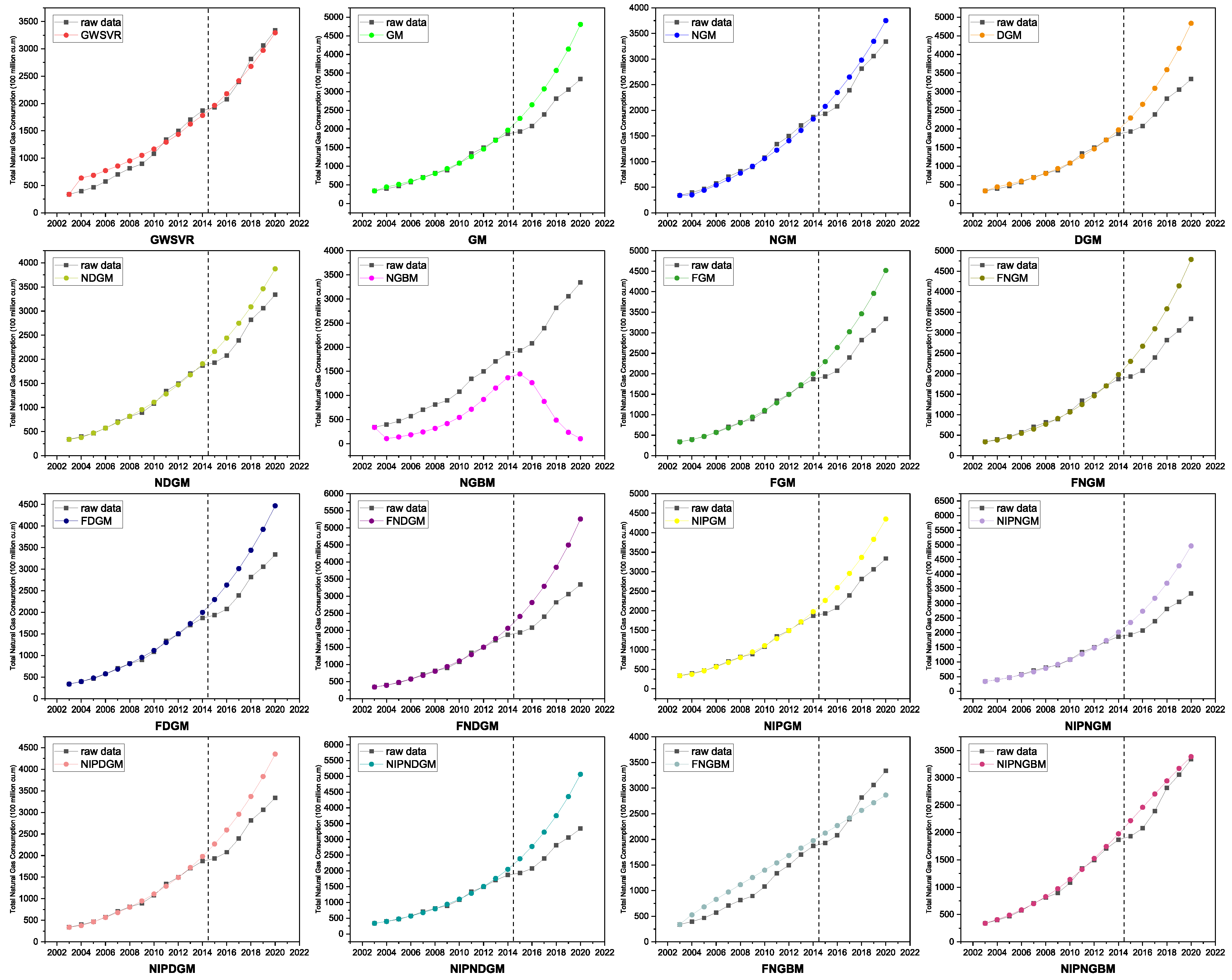
In the case of the total natural gas consumption forecasting, all the predicted values are shown in Figure 2, the selected optimal hyperparameters and training time of all models in Case II are listed in Table 5, and the out-of-sample metrics are listed in Table 6. Overall, the GWSVR (Grey Wolf Support Vector Regression) model demonstrates superior performance, with predicted values closely aligned with the raw data and outperforming the other benchmarked models. Notably, only the GWSVR model successfully captures the fluctuations observed from 2014, whereas the other models exhibit limitations in handling these fluctuations. Additionally, the GWSVR model excels in following the overall trend and exhibits minimal difficulty in out-of-sample forecasting, in contrast to the other models where the predicted values deviate significantly from the out-of-sample raw data. Notably, most other models exhibit poor performance, indicating overfitting issues. Conversely, the GWSVR model demonstrates enhanced capability in addressing inflection points when compared to the other models.
Based on the aforementioned discussion, the out-of-sample evaluation metrics presented in Table 6 provide empirical evidence supporting the superior performance of the GWSVR model compared to the other benchmarked grey system models in the natural gas time series forecasting. Specifically, the GWSVR model exhibits a significantly smaller MAPE compared to the benchmark models, with reductions ranging from 6.316363% to 63.820175%. Furthermore, the GWSVR model achieves a R 2 value of 0.974481, which stands in stark contrast to most other models that yield negative R 2 values. And the out-of-sample predictive capability of the other models is notably inferior, as evidenced by MAPE values exceeding 9%. In summary, the GWSVR model consistently demonstrates superior forecasting performance when compared to the other grey system models. The comprehensive out-of-sample forecasting results of all the models are presented in Table 7. The median error of the GWSVR model is lower from 197.28353% to 1912.94653% compared to other benchmarked models. Additionally, it is interesting to see that the maximum error of the GWSVR is three times less than the minimum error of the NGBM model. The NGBM model presents the worst performance in this case, as it is underfitting. In summary, the GWSVR model consistently demonstrates superior forecasting performance when compared to the other grey system models.

4.4. Discussion

For further discussion, it is evident that the GWSVR model consistently outperforms all other models in terms of having the most accurate out-of-sample predictions that closely align with the original data, as well as superior evaluation metrics compared to the benchmarked grey system models. More detailed analyses of the model’s predictive ability and application performance are provided below.

4.4.1. Comparisons of the GWSVR Model and Linear Grey System Models

In comparison to the linear grey system models, the GWSVR model exhibits notable superiority in this study. The MAPE of the GWSVR model is ten times smaller than that of the GM and DGM models in both cases. This contrast clearly highlights the limitations of linear models, which fail to capture the correct out-of-sample trends. Additionally, linear models struggle to handle inflection points, often producing predicted values that deviate from the raw data. In contrast, the GWSVR model demonstrates remarkable adaptability in addressing these challenges and consistently delivers stable performance across all cases. Its strength lies in effectively extracting temporal features while simultaneously processing time series characteristics.

4.4.2. Comparisons of the GWSVR Model and Nonlinear Grey System Models

In this work, the nonlinear grey system models have consistently gained the advantage over the linear grey system models in terms of natural gas consumption forecasting, and the forecasting comparisons and findings are consistent with the existing work in that the nonlinear grey system models always yield better forecasting performance than the linear grey system models. In comparison with the nonlinear grey system models, the NIPNGBM and FNGBM offer the smallest MAPEs of 9.316916% and 9.073488% in the benchmarked models, respectively, while the GWSVR provides MAPEs of 2.671638% and 2.757125%, respectively. On the other hand, the GWSVR model is more capable of reaching the inflection points and enhancing the predictive ability with predicted values tightly following the raw trend.

5. Conclusions

In this work, a Grey Wavelet Support Vector Regressor (GWSVR) was proposed, with detailed modeling procedures and computational algorithms presented. Two real-world case studies on forecasting the natural gas supply and consumption in China are carried out using GWSVR in comparison with 15 grey system models, including linear and nonlinear models. The results clearly indicate that most linear grey system models cannot perform well in these two cases, illustrating that the datasets are nonlinear. Although some existing nonlinear grey system models perform better than the linear models, their out-of-sample errors are significantly larger than those of GWSVR. Above all, the proposed model demonstrates higher performance than the other 15 existing grey system models, further indicating the eligibility of the proposed modeling method and algorithm for building accurate grey system models. Additionally, it can be observed that the MAPEs of GWSVR in both cases are smaller than 3%, indicating its high potential in forecasting the natural gas supply and demand in China based on recent historical datasets. The results of the applications suggest that the proposed GWSVR can serve as a reliable decision-making support tool in the future.

Author Contributions

Author Contributions: Conceptualization, methodology, writing—original draft preparation, writing—review and editing, software, funding acquisition, X.M.; writing—original draft preparation, writing—review and editing, software, H.Y. and Y.D. All authors have read and agreed to the published version of the manuscript.

Funding

This research was funded by the Humanities and Social Science Fund of the Ministry of Education of China (19YJCZH119) and the Natural Science Foundation of Sichuan Province (No. 2022NSFSC1821).

Data Availability Statement

Publicly available datasets were analyzed in this study. The data can be found here: https://data.stats.gov.cn/english/easyquery.htm?cn=C01.

Conflicts of Interest

Authors declare that there is no conflict of interest due to the publication of this paper.

References

  1. Liu, X.; Lin, Z.; Feng, Z. Short-term offshore wind speed forecast by seasonal ARIMA—A comparison against GRU and LSTM. Energy 2021, 227, 120492. [Google Scholar] [CrossRef]
  2. Bacanin, N.; Jovanovic, L.; Zivkovic, M.; Kandasamy, V.; Antonijevic, M.; Deveci, M.; Strumberger, I. Multivariate energy forecasting via metaheuristic tuned long-short term memory and gated recurrent unit neural networks. Inf. Sci. 2023, 642, 119122. [Google Scholar] [CrossRef]
  3. Al-Alimi, D.; AlRassas, A.M.; Al-qaness, M.A.; Cai, Z.; Aseeri, A.O.; Abd Elaziz, M.; Ewees, A.A. TLIA: Time-series forecasting model using long short-term memory integrated with artificial neural networks for volatile energy markets. Appl. Energy 2023, 343, 121230. [Google Scholar] [CrossRef]
  4. Dutta, R.; Das, S.; De, S. Multi criteria decision making with machine-learning based load forecasting methods for techno-economic and environmentally sustainable distributed hybrid energy solution. Energy Convers. Manag. 2023, 291, 117316. [Google Scholar] [CrossRef]
  5. Pawar, P.; Tarun Kumar, M.; Vittal, K.P. An IoT based Intelligent Smart Energy Management System with accurate forecasting and load strategy for renewable generation. Measurement 2020, 152, 107187. [Google Scholar] [CrossRef]
  6. Tayab, U.B.; Lu, J.; Yang, F.; AlGarni, T.S.; Kashif, M. Energy management system for microgrids using weighted salp swarm algorithm and hybrid forecasting approach. Renew. Energy 2021, 180, 467–481. [Google Scholar] [CrossRef]
  7. Cao, Y.; Liu, G.; Sun, J.; Bavirisetti, D.P.; Xiao, G. PSO-Stacking improved ensemble model for campus building energy consumption forecasting based on priority feature selection. J. Build. Eng. 2023, 72, 106589. [Google Scholar] [CrossRef]
  8. Deng, J. Control problems of grey systems. Syst. Control Lett. 1982, 1, 288–294. [Google Scholar] [CrossRef]
  9. Ding, S.; Tao, Z.; Zhang, H.; Li, Y. Forecasting nuclear energy consumption in China and America: An optimized structure-adaptative grey model. Energy 2022, 239, 121928. [Google Scholar] [CrossRef]
  10. Ding, S.; Li, R.; Wu, S.; Zhou, W. Application of a novel structure-adaptative grey model with adjustable time power item for nuclear energy consumption forecasting. Appl. Energy 2021, 298, 117114. [Google Scholar] [CrossRef]
  11. Zhao, H.; Wu, L. Forecasting the non-renewable energy consumption by an adjacent accumulation grey model. J. Clean. Prod. 2020, 275, 124113. [Google Scholar] [CrossRef]
  12. Luo, X.; Duan, H.; He, L. A Novel Riccati Equation Grey Model And Its Application In Forecasting Clean Energy. Energy 2020, 205, 118085. [Google Scholar] [CrossRef]
  13. El-Fouly, T.; El-Saadany, E.; Salama, M. Grey predictor for wind energy conversion systems output power prediction. IEEE Trans. Power Syst. 2006, 21, 1450–1452. [Google Scholar] [CrossRef]
  14. Şahin, U. Forecasting share of renewables in primary energy consumption and CO2 emissions of China and the United States under COVID-19 pandemic using a novel fractional nonlinear grey model. Expert Syst. Appl. 2022, 209, 118429. [Google Scholar] [CrossRef]
  15. Li, D.C.; Chang, C.J.; Chen, C.C.; Chen, W.C. Forecasting short-term electricity consumption using the adaptive grey-based approach—An Asian case. Omega 2012, 40, 767–773. [Google Scholar] [CrossRef]
  16. Hamzacebi, C.; Es, H.A. Forecasting the annual electricity consumption of Turkey using an optimized grey model. Energy 2014, 70, 165–171. [Google Scholar] [CrossRef]
  17. Wang, Q.; Song, X.; Li, R. A novel hybridization of nonlinear grey model and linear ARIMA residual correction for forecasting U.S. shale oil production. Energy 2018, 165, 1320–1331. [Google Scholar] [CrossRef]
  18. Ma, H.; Zhang, Z. Grey prediction with Markov-Chain for Crude oil production and consumption in China. In Proceedings of the The Sixth International Symposium on Neural Networks (ISNN 2009), New York, NY, USA, 2–5 August 2009; Springer: Berlin/Heidelberg, Germany, 2009; pp. 551–561. [Google Scholar]
  19. Chen, Y.; Yang, D.; Dai, W.Z. Modeling research of model GM (1,1) background value-building based on Gauss-Legendre quadrature and its application. J. Zhejiang Sci.-Tech. Univ. 2007, 4, 444–447. [Google Scholar]
  20. Xie, N.; Liu, S. Discrete GM(1,1) model and gray prediction modeling mechanism model. Syst. Eng. Theory Pract. 2005, 25, 93–99. [Google Scholar]
  21. Liu, B.; Zhao, L.; Zhai, Z.J.; Dang, Y.G.; Zhang, R. Optimum model of GM(1,1) and its suitable range. J. Nanjing Univ. Aeronaut. Astronaut. 2003, 35, 451–454. [Google Scholar]
  22. Cui, J.; Liu, S.F.; Zeng, B.; Xie, N.M. A novel grey forecasting model and its optimization. Appl. Math. Model. 2013, 37, 4399–4406. [Google Scholar] [CrossRef]
  23. Zhou, W.; Wu, X.; Ding, S.; Pan, J. Application of a novel discrete grey model for forecasting natural gas consumption: A case study of Jiangsu Province in China. Energy 2020, 200, 117443. [Google Scholar] [CrossRef]
  24. Yan, C.; Wu, L.; Liu, L.; Zhang, K. Fractional Hausdorff grey model and its properties. Chaos Solitons Fractals 2020, 138, 109915. [Google Scholar] [CrossRef]
  25. Qian, W.; Dang, Y.; Liu, S. Grey GM (1, 1, tα) model with time power and its application. Syst. Eng.-Theory Pract. 2012, 32, 2247–2252. [Google Scholar]
  26. Zeng, B.; Duan, H.; Zhou, Y. A new multivariable grey prediction model with structure compatibility. Appl. Math. Model. 2019, 75, 385–397. [Google Scholar] [CrossRef]
  27. Liu, X.; Moreno, B.; García, A.S. A grey neural network and input-output combined forecasting model. Primary energy consumption forecasts in Spanish economic sectors. Energy 2016, 115, 1042–1054. [Google Scholar] [CrossRef]
  28. Ma, X.; Lu, H.; Ma, M.; Wu, L.; Cai, Y. Urban natural gas consumption forecasting by novel wavelet-kernelized grey system model. Eng. Appl. Artif. Intell. 2023, 119, 105773. [Google Scholar] [CrossRef]
  29. Mirjalili, S.; Mirjalili, S.M.; Lewis, A. Grey wolf optimizer. Adv. Eng. Softw. 2014, 69, 46–61. [Google Scholar] [CrossRef] [Green Version]
  30. Cui, Y.; Jia, L.; Fan, W. Estimation of actual evapotranspiration and its components in an irrigated area by integrating the Shuttleworth-Wallace and surface temperaturevegetation index schemes using the particle swarm optimization algorithm. Agricultural and Forest Meteorology 2021, 307, 108488. [Google Scholar] [CrossRef]
  31. Mirjalili, S. Genetic algorithm. In Evolutionary Algorithms and Neural Networks: Theory and Applications; Studies in Computational Intelligence; Springer: Berlin/Heidelberg, Germany, 2019; Volume 780, pp. 43–55. [Google Scholar]
  32. Cai, Z.; Dai, S.; Ding, Q.; Zhang, J.; Xu, D.; Li, Y. Gray wolf optimization-based wind power load mid-long term forecasting algorithm. Comput. Electr. Eng. 2023, 109, 108769. [Google Scholar] [CrossRef]
  33. Heydari, A.; Garcia, D.A.; Keynia, F.; Bisegna, F.; Santoli, L.D. Renewable Energies Generation and Carbon Dioxide Emission Forecasting in Microgrids and National Grids using GRNN-GWO Methodology. Energy Procedia 2019, 159, 154–159. [Google Scholar] [CrossRef]
  34. Sebayang, A.; Kusumo, F.; Milano, J.; Shamsuddin, A.; Silitonga, A.; Ideris, F.; Siswantoro, J.; Veza, I.; Mofijur, M.; Reen Chia, S. Optimization of biodiesel production from rice bran oil by ultrasound and infrared radiation using ANN-GWO. Fuel 2023, 346, 128404. [Google Scholar] [CrossRef]
  35. Barman, M.; Dev Choudhury, N.B. A similarity based hybrid GWO-SVM method of power system load forecasting for regional special event days in anomalous load situations in Assam, India. Sustain. Cities Soc. 2020, 61, 102311. [Google Scholar] [CrossRef]
  36. Schölkopf, B.; Smola, A.J. Learning with Kernels: Support Vector Machines, Regularization, Optimization, and Beyond; MIT Press: Cambridge, MA, USA, 2002. [Google Scholar]
  37. Chen, P.H.; Fan, R.E.; Lin, C.J. A study on SMO-type decomposition methods for support vector machines. IEEE Trans. Neural Netw. 2006, 17, 893–908. [Google Scholar] [CrossRef] [PubMed] [Green Version]
  38. Xie, N.M.; Liu, S.F. Discrete grey forecasting model and its optimization. Appl. Math. Model. 2009, 33, 1173–1186. [Google Scholar] [CrossRef]
  39. Chen, C.I.; Chen, H.L.; Chen, S.P. Forecasting of foreign exchange rates of Taiwan’s major trading partners by novel nonlinear Grey Bernoulli model NGBM (1, 1). Commun. Nonlinear Sci. Numer. Simul. 2008, 13, 1194–1204. [Google Scholar] [CrossRef]
  40. Wu, L.; Liu, S.; Yao, L.; Yan, S.; Liu, D. Grey system model with the fractional order accumulation. Commun. Nonlinear Sci. Numer. Simul. 2013, 18, 1775–1785. [Google Scholar] [CrossRef]
  41. Duan, H.; Lei, G.R.; Shao, K. Forecasting crude oil consumption in China using a grey prediction model with an optimal fractional-order accumulating operator. Complexity 2018, 2018, 3869619. [Google Scholar] [CrossRef]
  42. Meng, W.; Yang, D.; Huang, H. Prediction of China’s sulfur dioxide emissions by discrete grey model with fractional order generation operators. Complexity 2018, 2018, 8610679. [Google Scholar] [CrossRef] [Green Version]
  43. Wu, L.F.; Liu, S.F.; Cui, W.; Liu, D.L.; Yao, T.X. Non-homogenous discrete grey model with fractional-order accumulation. Neural Comput. Appl. 2014, 25, 1215–1221. [Google Scholar] [CrossRef]
  44. Wu, L.; Liu, S.; Chen, H.; Zhang, N. Using a novel grey system model to forecast natural gas consumption in China. Math. Probl. Eng. 2015, 2015, 686501. [Google Scholar] [CrossRef] [Green Version]
  45. Cui, J.; Dang, Y.; Liu, S. Novel grey forecasting model and its modeling mechanism. Control Decis. 2009, 24, 1702–1706. [Google Scholar]
  46. Zhou, W.; Zhang, H.; Dang, Y.; Wang, Z. New information priority accumulated grey discrete model and its application. Chin. J. Manag. Sci. 2017, 25, 140–148. [Google Scholar]
  47. Xie, N.; Liu, S. Research on the non-homogenous discrete grey model and its parameter’s properties. Syst. Eng. Electron. 2008, 30, 863–867. [Google Scholar]
  48. Wu, W.; Ma, X.; Zeng, B.; Wang, Y.; Cai, W. Forecasting short-term renewable energy consumption of China using a novel fractional nonlinear grey Bernoulli model. Renew. Energy 2019, 140, 70–87. [Google Scholar] [CrossRef]
Figure 1. Predicted values of all models in Case I.
Systems 11 00428 g001
Figure 2. Predicted values of all models in Case II.
Systems 11 00428 g002
Table 1. Model performance metrics.
MetricsAbbreviationExpression
Mean Absolute ErrorMAE 1 n k = 1 n y 0 k y ^ 0 k
Mean Absolute Percentage ErrorMAPE 1 n k = 1 n y 0 k y ^ 0 k y k × 100 %
Mean Square ErrorMSE 1 n k = 1 n y 0 k y ^ 0 k 2
Root Mean Square ErrorRMSE 1 n k = 1 n y 0 k y ^ 0 k 2
Theil U Statistic 1U1 1 n k = 1 n y 0 k y ^ 0 k 2 1 n k = 1 n y 0 k 2 + 1 n k = 1 n y ^ 0 k 2
Theil U Statistic 2U2 1 n k = 1 n y 0 k y ^ 0 k 2 k = 1 n y 0 k 2
Median Absolute ErrorMedAe 1 n k = 1 n arctan y 0 k y ^ 0 k y k
Index of AgreementIA 1 k = 1 n y ( 0 ) ( k ) y ^ ( 0 ) ( k ) 2 k = 1 n y ( 0 ) ( k ) y ¯ ( 0 ) + y ^ ( 0 ) ( k ) y ^ ¯ ( 0 ) 2
Coefficient of DeterminationR 2 1 k = 1 n y 0 k y ^ 0 k 2 k = 1 n y 0 k y ¯ 0 2
Percent BiasPibas k = 1 n y 0 k y ^ 0 k k = 1 n y ^ 0 k
Table 2. Optimal hyperparameters and training times of the models in Case I.
ModelModel Abbreviation  Optimal Hyperparameters   Training Time (s)  
Grey Wavelet Support Vector RegressorGWSVRC = 279.8859, ν = 0.29200.84743 s
Nonhomogeneous Grey Bernoulli ModelNGBMn = 5.89440.03722 s
Fractional-order Grey ModelFGMr = 0.25820.15140 s
Fractional-order Nonhomogeneous Grey ModelFNGMr = 1.36830.09306 s
Fractional-order Discrete Grey ModelFDGMr = 0.23770.10684 s
Fractional-order Nonhomogeneous Discrete Grey ModelFNDGMr = −1.05250.61533 s
New Information Priority Grey ModelNIPGMr = 0.12180.05067 s
New Information Priority Nonhomogeneous Grey ModelNIPNGMr = 0.19560.05541 s
New Information Priority Discrete Grey ModelNIPDGMr = 0.81810.04859 s
New Information Priority Nonhomogeneous Discrete Grey ModelNIPNDGMr = 0.77220.19020 s
Nonlinear Grey Bernoulli Model with Fractional-order Accumulation   FNGBMn = 2.0000, r = −0.02550.78871 s
New Information Priority Nonlinear Grey Bernoulli ModelNIPNGBMn = 2.0000, r = 0.00000.42991 s
Table 3. Out-of-sample forecasting metrics of all models in Case I.
GWSVRGMNGMDGMNDGMNGBMFGMFNGMFDGMFNDGMNIPGMNIPNGMNIPDGMNIPNDGMFNGBMNIPNGBM
MAE67.67645838.3097248.2112856.624353.46561931.666681.2515634.3292671.4348375.5022720.99391633.579573.23321294.021294.8063213.4934
MAPE2.67163830.904739.52033931.597413.6329369.1508125.5732323.5201525.2475614.8020127.0187760.1794521.6845447.2095212.297869.316916
MSE6210.548851,978.171,475.37887,239.9136,967.94,851,922530,154.6480,953.7512,394.5146,942.1596,039.93,214,052368,567.42,103,85893,267.1457,426.36
RMSE78.80703923.0266267.3488941.9341370.09172202.708728.1172693.5083715.8174383.3302772.03621792.778607.09751450.468305.3967239.638
U10.0149780.149540.0483490.1521320.0656710.6284130.1215690.1165790.1197470.0678480.1279810.2549250.1034040.2170420.0549860.043823
U20.0298890.3500720.1013960.3572430.1403630.8354110.276150.2630240.2714850.1453840.2928070.6799390.2302510.5501120.1158260.090886
MedAe60.64835726.0962249.7691743.6731346.38442072.833599.266545.3121591.2506381.9754636.01321447.303502.2161114.763280.7869200.0508
IA0.9931180.6763580.9393490.669580.8934180.1952240.7391850.760970.7432860.8800730.7225820.4601590.7878130.5341520.9044160.933144
R20.974704−2.470210.708873−2.613830.442114−18.7624−1.15938−0.95898−1.087040.401488−1.42774−12.0912−0.50122−7.569260.6201120.766096
Pbias0.001949−0.24455−0.08746−0.24856−0.12012.935512−0.20827−0.19675−0.20589−0.12664−0.21778−0.3868−0.18123−0.33319−0.1022−0.07616
Table 4. Detailed results of the out-of-sample forecasting of all models in Case I.
YearRaw DataGWSVRErrorGMErrorNGMErrorDGMErrorNDGMErrorNGBMErrorFGMErrorFNGMError
201519251962.351−37.35112286.432−361.4322069.711−144.7112297.588−372.5882155.033−230.0331468.653456.34692281.862−356.8622209.65−284.65
20162080.52177.216−96.71592654.098−573.5982337.722−257.2222667.468−586.9682430.429−349.9291300.472780.02782614.386−533.8862546.322−465.822
20172390.72415.607−24.90713080.887−690.1872633.016−242.3163096.894−706.1942733.54−342.84761.29751629.4022989.801−599.1012929.592−538.892
20182814.32680.101134.19943576.305−762.0052958.369−144.0693595.452−781.1523067.156−252.856298.03572516.2643413.731−599.4313366.033−551.733
20193057.52973.55483.945614151.389−1093.893316.842−259.3424174.271−1116.773434.346−376.84693.054412964.4463892.534−835.0343863.137−805.637
20203270.23299.14−28.93954818.947−1548.753711.806−441.6064846.271−1576.073838.49−568.2926.68973243.514433.394−1163.194429.442−1159.24
Minimum Error −24.9071 361.4315 144.0692 372.5879 230.0328 456.3469 356.862 284.6495
Maximum Error 134.1994 1548.747 441.6064 1576.071 568.29 3243.51 1163.194 1159.242
Median Error −26.9233 −726.096 −249.769 −743.673 −346.384 2072.833 −599.266 −545.312
YearRaw DataFDGMErrorFNDGMErrorNIPGMErrorNIPNGMErrorNIPDGMErrorNIPNDGMErrorFNGBMErrorNIPNGBMError
201519252283.078−358.0782213.542−288.5422296.67−371.672658.937−733.9372246.545−321.5452434.458−509.4582241.281−316.2812206.928−281.928
20162080.52612.751−532.2512489.094−408.5942636.458−555.9583135.378−1054.882559.518−479.0182871.576−791.0762498.838−418.3382451.233−370.733
20172390.72984.317−593.6172783.428−392.7283020.962−630.2623706.396−1315.72909.279−518.5793398.486−1007.792759.741−369.0412694.717−304.017
20182814.33403.184−588.8843096.616−282.3163456.065−641.7654393.209−1578.913300.153−485.8534036.041−1221.743019.185−204.8852932.474−118.174
20193057.53875.457−817.9573428.723−371.2233948.427−890.9275221.795−2164.33736.97−679.474809.935−1752.443272.5−2153160.051−102.551
20203270.24408.021−1137.823779.811−509.6114505.582−1235.386223.96−2953.764225.133−954.9335751.83−2481.633515.492−245.2923373.759−103.559
Minimum Error 358.078 282.3156 371.6699 733.9373 321.5452 509.4581 204.8847 102.5506
Maximum Error 1137.821 509.6112 1235.382 2953.76 954.933 2481.63 418.3375 370.7326
Median Error −591.251 −381.975 −636.013 −1447.3 −502.216 −1114.76 −280.787 −200.051
Table 5. Optimal hyperparameters and training times of the models in Case II.
ModelModel AbbreviationOptimal HyperparametersTraining Time (s)
Grey Wavelet Support Vector RegressorGWSVRC = 48.9141, ν = 0.29070.78489 s
Nonhomogeneous Grey Bernoulli ModelNGBMn = 4.21620.03195 s
Fractional-order Grey ModelFGMr = 0.15050.08470 s
Fractional-order Nonhomogeneous Grey ModelFNGMr = 1.09020.08795 s
Fractional-order Discrete Grey ModelFDGMr = 0.13540.08445 s
Fractional-order Nonhomogeneous Discrete Grey ModelFNDGMr = 0.76100.22519 s
New Information Priority Grey ModelNIPGMr = 0.84930.04955 s
New Information Priority Nonhomogeneous Grey ModelNIPNGMr = 0.98390.05257 s
New Information Priority Discrete Grey ModelNIPDGMr = 0.84810.04881 s
New Information Priority Nonhomogeneous Discrete Grey ModelNIPNDGMr = 0.90300.18856 s
Nonlinear Grey Bernoulli Model with Fractional-order AccumulationFNGBMn = 2.0000, r = −1.09850.77943 s
New Information Priority Nonlinear Grey Bernoulli ModelNIPNGBMn = 2.0000, r = 0.00000.42851 s
Table 6. Out-of-sample forecasting metrics of all models in Case II.
GWSVRGMNGMDGMNDGMNGBMFGMFNGMFDGMFNDGMNIPGMNIPNGMNIPDGMNIPNDGMFNGBMNIPNGBM
MAE70.73226819.5432257.3194837.7925360.08071867.335715.0994829.0862693.19671083.294625.0661933.0845626.1443992.5079245.9249212.6661
MAPE2.75712530.100739.85197830.7874413.8497966.577326.702830.5758325.9622439.781823.4672934.3975923.5206836.612669.0734889.362476
MSE6665.947803908.873997.96838135.1139421.44511417579693.9809827.3540108.11399142436994.91025289437770.2115670980026.3859962.91
RMSE81.64525896.6096272.0257915.4972373.39182124.01761.3763899.9041734.92051182.853661.05591012.566661.64211075.504282.8893244.8732
U10.0154690.1450060.0488330.1476060.0658070.5992540.1256890.1453970.121830.1829140.1109270.1607050.1110120.169010.0548370.044542
U20.0307740.3379510.1025320.345070.1407390.8005840.2869790.3391930.2770070.4458420.2491660.3816570.2493870.405380.1066270.092298
MedAe65.08349718.5948264.3201736.1083358.61981922.922639.5297735.5087620.9857963.1634558.1595831.6983559.5865886.4476221.2416207.2592
IA0.9928390.6950520.940510.6882520.8968170.2139420.73580.6916610.7446240.6053040.7740060.6541430.7734040.6338790.8668510.932628
R20.974481−2.077610.716713−2.208640.466251−16.2711−1.21925−2.10027−1.0677−4.35635−0.67295−2.92513−0.67592−3.428240.6936340.770443
Pbias0.00705−0.23943−0.08995−0.24346−0.121512.536972−0.21549−0.24154−0.21028−0.29384−0.19361−0.26385−0.19388−0.276010.044384−0.07552
Table 7. Detailed results of the out-of-sample forecasting of all models in Case II.
YearRaw DataGWSVRErrorGMErrorNGMErrorDGMErrorNDGMErrorNGBMErrorFGMErrorFNGMError
20151931.81964.998−33.19842284.76−352.962078.055−146.2552295.869−364.0692161.222−229.4221445.775486.02552298.388−366.5882304.295−372.495
20162078.12179.253−101.1532651.476−573.3762349.998−271.8982664.793−586.6932440.45−362.351266.439811.66082639.455−561.3552673.058−594.958
20172393.72416.87−23.16983077.053−683.3532650.442−256.7423093−699.32748.59−354.89876.43951517.2613025.939−632.2393097.102−703.402
20182817.12680.395136.7053570.937−753.8372982.374−165.2743590.016−772.9163088.635−271.535488.5172328.5833463.921−646.8213584.716−767.616
20193059.72972.65487.046224144.092−1084.393349.095−289.3954166.898−1107.23463.889−404.189234.89742824.8033960.299−900.5994145.432−1085.73
20203339.93296.77943.120774809.242−1469.343754.251−414.3514836.479−1496.583877.998−538.098104.22383235.6764522.894−1182.994790.215−1450.32
Minimum Error −23.1698 −352.96 −146.255 −364.069 −229.422 486.0255 −366.588 −372.495
Maximum Error 136.705 −1469.34 −414.351 −1496.58 −538.098 3235.676 −1182.99 −1450.32
Median Error 9.975466 −718.595 −264.32 −736.108 −358.62 1922.922 −639.53 −735.509
YearRaw DataFDGMErrorFNDGMErrorNIPGMErrorNIPNGMErrorNIPDGMErrorNIPNDGMErrorFNGBMErrorNIPNGBMError
20151931.82298.021−366.2212408.667−476.8672266.683−334.8832354.288−422.4882269.313−337.5132388.746−456.9462122.463−190.6632218.179−286.379
20162078.12633.393−555.2932814.976−736.8762591.951−513.8512737.896−659.7962594.262−516.1622778.55−700.452269.559−191.4592462.651−384.551
20172393.73012.31−618.613290.358−896.6582957.806−564.1063181.093−787.3932959.606−565.9063230.151−836.4512417.44−23.73982706.616−312.916
20182817.13440.461−623.3613846.769−1029.673369.313−552.2133693.104−876.0043370.367−553.2673753.544−936.4442566.076251.02422945.239−128.139
20193059.73924.275−864.5754498.21−1438.513832.167−772.4674284.585−1224.883832.191−772.4914360.338−1300.642715.438344.2623174.102−114.402
20203339.94471.02−1131.125261.082−1921.184352.777−1012.884967.842−1627.944351.427−1011.535064.019−1724.122865.499474.40093389.509−49.6092
Minimum Error −366.221 −476.867 −334.883 −422.488 −337.513 −456.946 −23.7398 −49.6092
Maximum Error −1131.12 −1921.18 −1012.88 −1627.94 −1011.53 −1724.12 474.4009 −384.551
Median Error −620.986 −963.163 −558.16 −831.698 −559.586 −886.448 113.6422 −207.259
Disclaimer/Publisher’s Note: The statements, opinions and data contained in all publications are solely those of the individual author(s) and contributor(s) and not of MDPI and/or the editor(s). MDPI and/or the editor(s) disclaim responsibility for any injury to people or property resulting from any ideas, methods, instructions or products referred to in the content.