Article

Modeling a Carbon-Efficient Road–Rail Intermodal Routing Problem with Soft Time Windows in a Time-Dependent and Fuzzy Environment by Chance-Constrained Programming

1
School of Management Science and Engineering, Shandong University of Finance and Economics, Jinan 250014, China
2
School of International Trade and Economics, Shandong University of Finance and Economics, Jinan 250014, China
3
SDU-ANU Joint Science College, Shandong University, Weihai 264209, China
*
Author to whom correspondence should be addressed.
Systems 2023, 11(8), 403; https://doi.org/10.3390/systems11080403
Submission received: 6 July 2023 / Revised: 2 August 2023 / Accepted: 4 August 2023 / Published: 6 August 2023

Abstract

:
This study explores a road–rail intermodal routing problem. To improve the carbon efficiency of transportation, reducing CO2 emissions is considered by the routing. Soft time windows are incorporated into the routing to optimize the timeliness of the first-mile pickup and last-mile delivery services in intermodal transportation. The routing is further modeled in a time-dependent and fuzzy environment where the average truck speeds of the road depend on the truck departure times and are simultaneously considered fuzzy along with rail capacities. The fuzzy truck speed leads to the fuzziness of three aspects, including speed-dependent CO2 emissions of the road, a timetable-constrained transfer process from road to rail, and delivery time window violation. This study formulates the routing problem under the above considerations and carbon tax regulation as a combination of transportation path planning problem and truck departure time and speed matching problem. A fuzzy nonlinear optimization model is then established for the proposed routing problem. Furthermore, chance-constrained programming with general fuzzy measure is used to conduct the defuzzification of the model to make the problem solvable, and linearization techniques are adopted to linearize the model to enhance the efficiency of problem-solving. Finally, this study presents an empirical case to demonstrate the effectiveness of the designed approach. This case study evaluates the performance of carbon tax regulation by comparing it with multi-objective optimization. It also focuses on sensitivity analysis to discuss the influence of the optimistic–pessimistic parameter and confidence level on the optimization results. Several managerial insights are revealed based on the case study.

1. Introduction

The transportation industry plays a vital role in supporting China’s economic and social development. Currently, China has been in an unreasonable road-dominated transportation structure for a long time, which not only reduces transportation efficiency but also contributes to a large amount of energy consumption and CO2 emissions that considerably harm environmental quality and sustainability [1,2]. To achieve energy conservation and environmental protection in the transportation sector, China is promoting a modal shift policy to motivate the change of long-haul goods transportation from road to rail [3]. The modal shift policy aims to increase the proportion of railways in long-haul goods transportation and establish a reasonable transportation structure that can effectively combine road and rail transportation. To implement the policy and achieve efficient and green transportation, developing road–rail intermodal transportation (RRIT) is being attached to great importance by the transportation industry. RRIT uses road transportation that has the advantages of high flexibility and mobility and simplified maintenance for short/medium-distance pickup and delivery activities and adopts rail transportation, which is a cost-effective and energy-saving means for long-haul transportation [4,5]. Coordinating road and rail to realize intermodality can integrate their respective advantages and make RRIT a more excellent competitor to road transportation.
Improving the performance of the operations of intermodal transportation can provide the best door-to-door transportation service for shippers and receivers, which can attract more freight sources from the road and naturally optimize the transportation structure. Customer-centric and operational-level routing is critical to enhancing the economy, timeliness, and reliability of transportation [6]. By selecting the most suitable road and rail services and coordinating them through intermodal transfer, routing optimization can plan the optimum origin-to-destination routes to accomplish transportation orders. Consequently, intermodal routing has been acknowledged as a highlight in the transportation planning field [7]. Furthermore, carbon-efficient routing can balance the environmental sustainability concerned with lowering CO2 emissions and other objectives, which can enable the RRIT to reach its full potential as an environmentally friendly means of transportation and help to enhance the environmental goal of the road-to-rail modal shift policy.
This study is interested in a carbon-efficient road–rail intermodal routing problem (RRIRP). As a widely used low-carbon policy, carbon tax regulation is adopted to deal with CO2 emissions, and its performance should be estimated by comparing it with multi-objective optimization. The timeliness of pickup and delivery services expected by shippers and receivers are represented by soft time windows such that the time window violation is allowed and penalized to improve customer service flexibility that could be beneficial to other objectives. The proposed RRIRP aims to minimize the total costs, including transportation costs, emission costs, and penalty costs. The cost objective reflects a combination of economy, environmental sustainability (carbon efficiency), and timeliness of transportation. The minimization of the cost objective of the RRIRP shows a balance among these considerations.
Furthermore, the RRIRP should be studied in a real-world transportation scenario to ensure that the coordination of road and rail can be realized by RRIRP in the actual transportation. In real-world transportation, the operations of rail services (specifically, in this study, container block trains) follow fixed timetables [8], while road services (specifically, in this study, container trucks) are flexible [9]. Coordinating road and rail by RRIRP to enhance intermodality and accomplish transportation orders should fully model the above differences. Besides the differences in the operations, the two transportation modes are in different environments. Rail services are in a stable environment and are less influenced by the surroundings. The travel time of a container block train is fixed and determined by the departure and arrival times that are regulated by the train’s timetable. However, road services are easily affected by many factors, such as accidents, bad weather, drivers’ behaviors, road type, and time-varying traffic density [10]. Consequently, the truck speed of road service varies in different time ranges of the day and depends on the time when the trucks depart from the node. Therefore, road services yield time-dependent truck speeds. Since the CO2 emissions of the road mainly depend on speed, the time dependency of truck speeds leads to the time-dependent emission rates of the road [11].
In advanced RRIRP, it is difficult to predict the exact and real-time truck speeds due to the constantly changing background traffic conditions and influencing factors that are not known with certainty [12]. Therefore, the truck speed of road service in a time range is considered uncertain. The truck speed uncertainty leads to the uncertainty of three aspects, including the emission rates of road, the transfer process from road to rail, and delivery time window violation. Additionally, the capacity of a container block train cannot be fully saved for the containers of the targeted transportation orders and could be occupied by other transportation tasks that are also difficult to be accurately predicted in advance since there is not enough information [13]. Accordingly, the rail capacities are also uncertain in the advanced optimization phase. In most cases, there is a lack of enough data to fit the probability distributions of speeds and capacities, which limits the feasibility of stochastic programming [14]. In addition, using large numbers of scenarios to represent uncertainty increases the computational complexity of stochastic programming models [15]. Consequently, this study uses fuzzy trapezoidal numbers to describe the uncertainty and takes advantage of fuzzy programming to deal with the RRIRP.
Formulation of uncertainty is a promising way to achieve reliable transportation planning [16]. The carbon-efficient RRIRP should capture the time-dependent and fuzzy environment to improve its practical feasibility. Enabled by the time flexibility of the road, this study models a truck departure time and speed matching problem and integrates it into the RRIRP to further improve the operations of the road sector in the intermodality. Such matching can improve the efficiency and reliability of the transfer between road and rail in a fuzzy environment, reduce road emissions, and lower the time window violation. Meanwhile, this study will model the constraints of the fixed timetables of rail services on the transfer between road and rail.
The remaining sections of this study are organized as follows. The relevant literature is reviewed in Section 2 to understand the research progress on the topic discussed in this study, summarize the current research gaps, and clarify the contributions of this study. Section 3 gives the background information that should be known in advance, and a brief introduction to the specific RRIRP explored in this study is presented at the end of this section. In Section 4, a fuzzy nonlinear optimization model is established to deal with the proposed RRIRP. In Section 5, a solution approach combining chance-constrained programming (CCP) and model linearization is developed to enable the proposed RRIRP to be solved efficiently. Section 6 presents an empirical case study to demonstrate the effectiveness of the proposed approach. In this section, the performance of carbon tax regulation is evaluated by comparing it with multi-objective optimization. The sensitivity of the optimization results concerning the optimistic–pessimistic parameter and confidence level is also analyzed to find some managerial insights and demonstrate the advantages of the proposed CCP model. Finally, this study draws conclusions in Section 7.

2. Literature Review

Studies on the carbon-efficient intermodal routing problem (also known as green routing or environmental routing) have been very prevalent in recent years and indicate a wide adoption of carbon tax regulation to improve the carbon efficiency of routing. Chang et al. [17] took carbon emission costs under tax regulation as the external costs of truck–sea intermodal transportation and proposed a carbon-efficient truck–sea shortest path problem. Zhang et al. [18] discussed the mode choice problem for carbon-efficient intermodal transportation and built an integer programming model considering the minimization of the logistics costs and carbon tax. Guo et al. [19] considered a carbon-efficient intermodal routing problem with flexible truck departure times under travel time stochasticity and gave a CCP formulation that adds carbon tax to its cost objective. Duan and Heragu [20] analyzed the effects of carbon tax regulation in intermodal routing by sensitivity analysis and found carbon tax rates that can reduce emissions without increasing transportation costs. Zhang et al. [21] presented a carbon-efficient multimodal routing problem with hard time windows and concluded that the emission reduction achieved by carbon tax regulation is influenced by the setting of the time windows. Chen et al. [22] compared the carbon tax and trading regulations in intermodal route decisions and pointed out that the emission reduction of carbon trading regulation is less than that of carbon tax regulation. The same conclusion has also been found by Sun [6] in a carbon-efficient intermodal routing problem considering truck speed selection and multiple time windows.
Apart from Sun [6], the above studies realized the carbon tax-driven emission reduction through a single transportation path modification that replaces the high-emission transportation services with low-emission ones. However, they neglected the use of speed optimization to further improve the carbon efficiency of carbon tax regulation in the routing. Speed is extensively known as the key influencing factor that determines the emission rates of transportation modes [23]. In intermodal transportation, the operations of rail services are restricted by fixed timetables. Thus, the speed optimization for rail services is restricted. On the contrary, truck speed is controllable and departure time is flexible. Therefore, truck speed optimization is applicable, which has already been acknowledged by vehicle routing problems (VRP). Currently, there are a limited number of relevant studies on carbon-efficient intermodal routing problems considering speed optimization. Sun [6] proposed a discrete truck speed option model and explored a carbon-efficient intermodal routing problem integrating a truck speed selection decision that aims to further reduce the emissions of roads. The case study in this work demonstrated that truck speed optimization can achieve improved carbon efficiency of intermodal routing. Moreover, Ji and Wu [24] studied a multi-objective optimization for the carbon-efficient truck–sea intermodal routing problem, in which the truck speeds with lower and upper limits are considered as continuous variables and optimized to reduce fuel consumption and CO2 emissions. Resat and Turkay [25] also formulated truck speed optimization to avoid traffic congestion, but their work on the optimization of the intermodal transportation network did not take emission reduction into account. In addition, some studies simply focus on speed optimization for intermodal transportation, e.g., Kontovas and Psaraftis [26] and Fan et al. [27].
The above intermodal routing studies considering truck speed optimization neglected the time dependency of truck speeds that exists in the real world. As indicated by large numbers of green VRP studies, e.g., [10,11,28,29,30], it is meaningful to explore the green VRP integrating time-dependent truck speeds that enable speed optimization to reduce CO2 emissions and (or) fuel consumptions and better satisfy soft or hard time window constraints. Compared with the VRP with time-dependent speeds, studies on intermodal routing considering such a characteristic are pretty limited. Braekers et al. [31] modeled a time-dependent routing of drayage operations in the service area of intermodal terminals, in which the time-dependent speeds are converted into time-dependent travel times. Although discussed in an intermodal transportation setting, their work is still a VRP.
Currently, time-dependent intermodal routing studies primarily focus on time-dependent travel times. Zhang et al. [9] modeled the time dependency of truck travel times as a piecewise linear function and investigated a carbon-efficient intermodal routing problem with soft pickup and delivery time windows and road service flexibility. Sun et al. [32] and Guo et al. [33] considered the same modeling of time dependency as Zhang et al. [9] and presented an intermodal routing problem in a dynamic environment and a multimodal routing problem with traffic congestion and capacity uncertainty, respectively. In these studies, the formulation of time-dependent travel times contributes to optimizing the efficiency of intermodal transfer and timeliness regarding time windows or due dates. However, the emission rates of road services are not influenced by such a time dependency in their studies. Moreover, their routing optimization is formulated under travel time certainty. As a result, the truck departure time and travel time matching under their routing considerations cannot achieve improvement in the carbon efficiency and reliability of intermodal transportation.
Compared with the extensive understanding of the time-dependent truck speeds in VRP, only a few VRP researchers paid attention to the truck speed uncertainty. Nasri et al. [12] analyzed the reasons that lead to truck speed uncertainty and proposed the pollution-routing problem for autonomous trucks under speed uncertainty. Considering the stochasticity of truck speeds, the authors developed a two-stage stochastic programming model that employs scenarios to represent uncertainty. Teng et al. [34] assumed that the vehicle speeds follow normal distributions and modeled a bi-objective reliable eco-routing problem under uncertainty and fuel consumption. Sandamali et al. [35] fitted probability distributions of uncertain speeds of aircraft and addressed a flight routing and scheduling problem under uncertainty and fuel consumption by formulating a stochastic programming model. To the best of our knowledge, existing studies on unimodal routing or intermodal routing have not comprehensively explored the time dependency and uncertainty of speeds of the road or other transportation modes, which also results in the time dependency and uncertainty of the speed-dependent emission rates of transportation modes (especially road) being ignored by the routing literature, as well as the resulting uncertainty of the transfer from road to rail that only exists in intermodal routing. Currently, only Sun [36] and Sun et al. [37] discussed the uncertainty of intermodal transfer caused by demand uncertainty and travel time uncertainty, respectively.
Contrary to the less attention to speed uncertainty, recent intermodal routing studies attached importance to capacity uncertainty. A group of articles by Sun et al. [6,32,36,37] describe triangular/trapezoidal fuzzy capacities and constructed fuzzy chance-constrained intermodal routing models. Lu et al. [38] presented a Eurasian multimodal routing model that considers the fuzziness of both time and capacity and developed a triangular fuzzy CCP model. Unlike the above studies, Uddin and Huynh [39] studied capacity stochasticity in a reliable RRIRP. All intermodal routing studies emphasized the significant influence of capacity uncertainty on the reliability and other objectives of routing optimization. Recent review studies highlighted intermodal routing under uncertainty as a noteworthy and emerging research domain [16,40] and further emphasized the significance of modeling uncertainty in the supply chain management field [41]. However, this study finds that the combination of speed uncertainty and capacity uncertainty is not a concern in the existing research. Actually, the majority of the intermodal routing literature still focuses on deterministic environments. Besides the single-objective setting, many articles on deterministic intermodal routing discussed multi-objective optimization problems considering at least two goals oriented on the economy (as the primary goal), timeliness (e.g., [42,43]), risk (e.g., [44,45]), and sustainability (e.g., [46,47]), etc., and obtained the Pareto solutions to balance the objectives conflicting with each other. Modeling transportation modes is also concerned by deterministic intermodal routing studies, in which some transportation modes are modeled with fixed departure times (e.g., [48,49]), fixed service time windows (e.g., [42,50,51]), or fixed timetables/schedules covering the above parameters (e.g., [52]); meanwhile, the flexibility of some transportation modes starts to receive consideration [9]. To formulate the deterministic intermodal routing problems, researchers proposed optimization models using pure 0–1 integer programming (e.g., [53]), mixed 0–1 integer programming (e.g., [50,52]), linear programming (e.g., [17]), and nonlinear programming (e.g., [44,52]). Solution methods developed by relevant studies include two types, i.e., exact solution methods (e.g., [17,44,52,54]) and heuristic algorithms (e.g., [42,49,50]). All these deterministic intermodal routing studies provide insights for our study in problem formulation and method design.
Finally, intermodal routing with time windows is a foundational research direction in which time windows are adopted to avoid earliness and lateness and seek on-time transportation. In recent years, the formulation of time windows has changed from hard time windows to soft time windows and from delivery time windows to pickup and delivery time windows [9,37]. Using soft time windows, pickup and delivery services are allowed and penalized for violating the time windows to a certain degree, by which customer service flexibility can be enhanced. The existing literature proposed a piecewise linear penalty cost function to deal with the soft time windows in a deterministic environment. In our study, the pickup start time is a deterministic variable. However, the truck speed uncertainty leads to a delivery accomplishment time uncertainty. In this case, the pickup time windows are in a deterministic environment, but the delivery time windows should address the time uncertainty. It is impossible to determine exactly whether the uncertain time violates the lower or upper bound of a soft time window. Consequently, the traditional piecewise linear function is infeasible for modeling penalty costs regarding soft delivery time windows under uncertainty. However, current studies paid less attention to the modeling of soft time windows under uncertainty. Only Sun’s work on intermodal routing [36] formulated the fuzzy environment of the soft delivery time windows that are caused by the demand fuzziness of transportation orders. However, Sun’s study [36] assumed that the pickup services start at fixed time points and only considered soft delivery time windows.
Above all, although solid research progress has been achieved by the existing studies on intermodal routing, there are still some research gaps that need to be bridged by this study:
(1)
Although carbon tax regulation has been widely used in carbon-efficient intermodal routing studies, the carbon tax rate is usually a constant in these studies, and the performance and feasibility of carbon tax regulation are rarely estimated in their case analysis.
(2)
Moreover, under carbon tax regulation, emission reduction is simply driven by transportation path modification in the current research, which limits the effective improvement of the carbon efficiency of the intermodal routing.
(3)
Time dependency and uncertainty of truck speeds are the natural characteristics of the road but are not fully modeled in the current studies. Ignoring the time-dependent truck speeds limits the diversity of approaches that can drive the emission reduction of the routing.
(4)
Although capacity uncertainty has been explored, the combination of speed uncertainty and capacity uncertainty that can achieve improved reliability of routing is not considered in the current studies.
(5)
The uncertainty of the transfer from road to rail caused by truck speed uncertainty is rarely modeled, which affects the reliability of the intermodal transfer of the routing optimization. Moreover, soft time windows in an uncertain environment resulting from truck speed uncertainty are not well established by existing studies.
To overcome the weaknesses of the current research, this study continues to investigate the carbon-efficient RRIRP by making the following contributions:
(1)
A carbon-efficient RRIRP is modeled in a time-dependent and fuzzy environment in which the time-dependent truck speeds of the road enable a truck departure time and speed matching to further strengthen the economy, carbon efficiency, timeliness, and reliability of the optimization.
(2)
Under carbon tax regulation, the carbon emission reduction in our model is driven by transportation path modification and truck departure time and speed matching. The feasibility of carbon tax regulation is verified by comparing it with multi-objective optimization in the empirical case study.
(3)
Multiple sources of uncertainty are incorporated into the RRIRP, including truck speeds and rail capacities. The induced system uncertainty is comprehensively formulated in the RRIRP, including speed-dependent emission rates of roads, transfer from road to rail, and violation of soft delivery time windows.
(4)
A CCP model with general fuzzy measure is employed to deal with the proposed RRIRP and provides decision-makers with the optimum solutions with reference to their attitudes on the objective and constraints.

3. Background Information

In this section, first of all, we establish a transportation system based on a real-world scenario where routing optimization will be used to organize the actual transportation. Then, we model a time-dependent and fuzzy environment to improve the feasibility of the RRIRP. Finally, we introduce the problem formulation for the proposed RRIRP.

3.1. Establishing the Transportation System

Considering their respective advantages, rail services are suitable to undertake long-haul transportation between intermodal terminals, and road services are beneficial for pickups from shippers to intermodal terminals and deliveries from intermodal terminals to receivers. Consequently, a three-phase RRIT using a hub-and-spoke structure can realize the door-to-door transportation of containers to meet customer demands.
In transportation, the drayage operators operate the pickup and delivery services, and the network operators manage the long-haul transportation using rail. The terminal operators conduct the transfer between road and rail. The intermodal operator represents the customers (i.e., shippers and receivers) and is concerned with operational-level routing optimization by cooperating with other operators and considering customer demands [55]. Consequently, the decision-makers involved are the intermodal operator and the customers. In this study, we assume that the intermodal operator can rent enough container trucks for drayage operators to pick up and deliver containers [50]. Therefore, road services are not constrained by capacities.
Additionally, truck-only transportation from shippers to receivers is still needed in the transportation system since it is more feasible than intermodality for transportation orders with tight due dates. Under the above considerations, the transportation network illustrated in Figure 1 is proposed for the RRIRP. Such a network structure has been widely used in intermodal transportation planning [32,37,55,56].
Furthermore, coordinating road and rail in the operational-level intermodal routing should be based on the practical operations of the two transportation modes. Therefore, the RRIRP should consider the time flexibility of roads and the fixed timetable of rail to ensure that the transportation using the planned routes is applicable in the real world. We also assume that the road services have fixed routes, while their departure times are optimizable.
Contrary to the time flexibility of the road, the timetable of a container block train includes the train’s departure times, arrival times, and loading/unloading operation time windows at different nodes on its fixed route as well as its running period [36,37]. The process of the three-phase RRIT is explained in Figure 1 and matches the time flexibility of the road and the fixed timetable of rail. The RRIRP should capture such a transportation process to enable the optimization results to be applicable in practice.

3.2. Modeling the Time-Dependent and Fuzzy Environment

3.2.1. Modeling of the Time-Dependent and Fuzzy Truck Speed

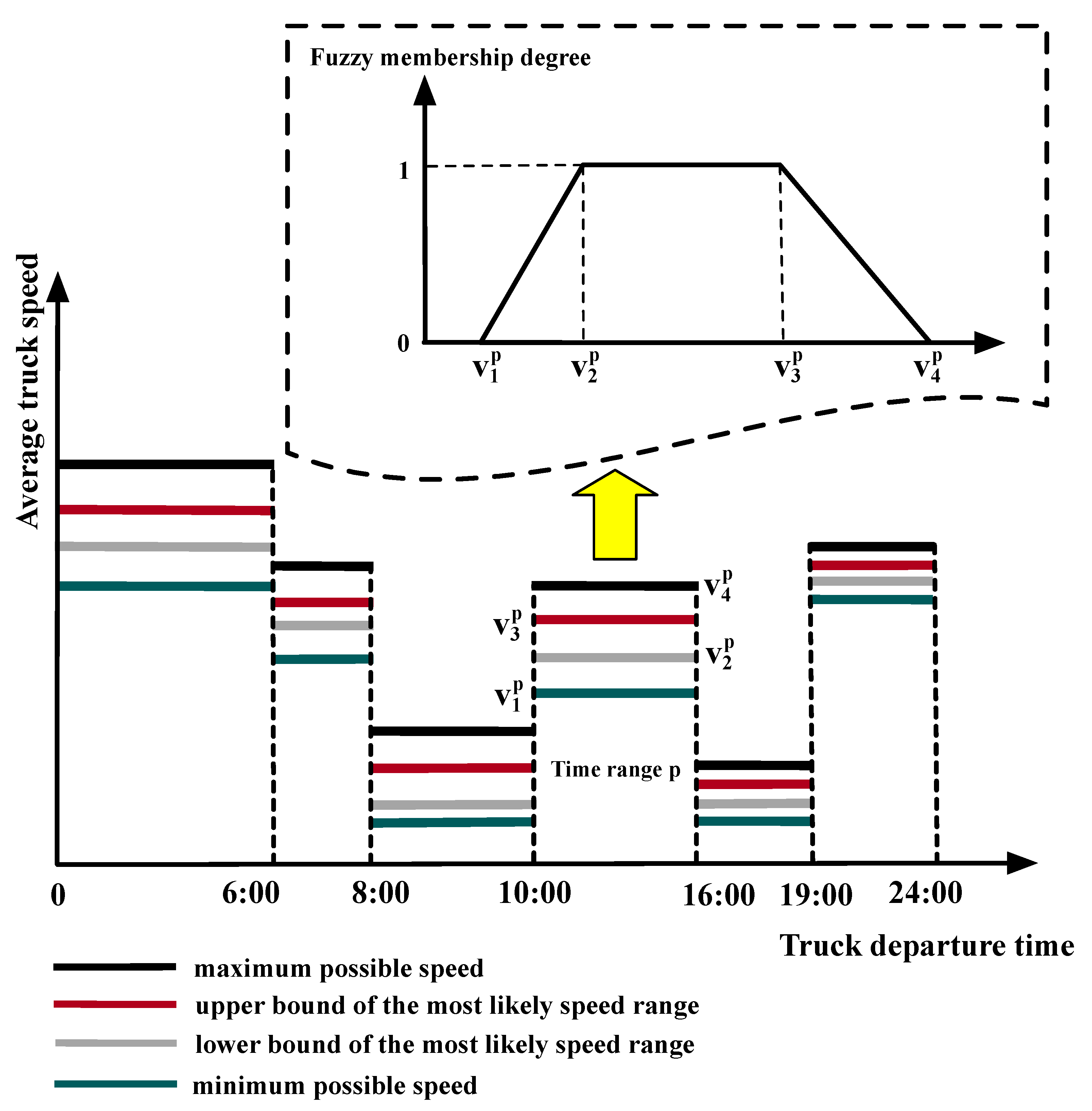
This study defines truck speed as the average speed of the trucks of a road service when carrying out pickup, delivery, or truck-only transportation. It depends on the truck departure time that can be optimized to enhance the optimization of the RRIRP. It should be noted that the determination of the average truck speed has considered the truck drivers’ rest en route that is requested to avoid fatigue driving. As claimed in Section 1, the truck speed has the characteristics of both time dependency and fuzziness. In this study, we use the staircase function to formulate the variation of the truck speed concerning the time ranges that the truck departure time falls into. Then, the speed in each time range is considered fuzzy. Trapezoidal fuzzy numbers are employed to formulate the fuzziness of the speed due to the higher flexibility of trapezoidal fuzzy numbers than the widely used triangular ones in modeling uncertain phenomena [36]. Therefore, the time-dependent and fuzzy truck speed is demonstrated in Figure 2.
As indicated by Figure 2, the fuzzy truck speed for road service in time range p can be expressed by a trapezoidal fuzzy number v 1 p ,   v 2 p ,   v 3 p ,   v 4 p where v 4 p v 3 p v 2 p v 1 p . v 1 p is the minimum possible truck speed in time range p and reflects the worst traffic condition of this time range. v 2 p ,   v 3 p is the most likely truck speed range in time range p representing the truck speeds in most cases of this time range, and when v 2 p = v 3 p , we can have a triangular fuzzy speed. v 4 p is the maximum possible truck speed in time range p and shows its best traffic condition. By using v 1 p ,   v 2 p ,   v 3 p ,   v 4 p , we can fully cover all the conditions that road service faces in a specific time range. Similarly, the fuzzy rail capacities can be described by the same type of fuzzy numbers, i.e., ϖ 1 ,   ϖ 2 ,   ϖ 3 ,   ϖ 4 where ϖ 1 is the minimum possible capacity of rail service, ϖ 2 ,   ϖ 3 is its most likely capacity range, ϖ 4 is the maximum possible capacity, and ϖ 4 ϖ 3 ϖ 2 ϖ 1 .
The truck speed of the road has limits. Wang et al. [57] stress that the average truck speed on the road in intermodal transportation is 47.5 km/hr. Li et al. [58] set the truck speed as 70 km/hr in intermodal transportation. Yang et al. [59] reveal that in intermodal transportation from China to the Indian Ocean, the average truck speed on the road from Shanghai to Kunming is 33.4 km/hr in a distance of 3207 km and that from Shenzhen to Kunming is 23.7 km/hr in a distance of 1706 km. Wang et al. [10] and Zhang et al. [28] analyze the real-world distribution of the speed of trucks in a day for the VRP and find that the truck speed falls into the range of [24, 68] km/hr and [20, 40] km/hr, respectively. Therefore, with reference to the above literature, this study considers a limit of [20, 70] km/hr for the average truck speeds of road services, i.e., v 1 p 20 km/hr and v 4 p 70 km/hr for p .

3.2.2. Modeling of the Induced System Fuzziness Resulting from Fuzzy Truck Speed

Modeling of the Speed-Dependent and Fuzzy CO2 Emissions of Road

CO2 emissions from roads are significantly influenced by truck speed [23]. Modeling the speed-dependent emissions enables the truck departure time and speed matching problem to consider the improvement of carbon efficiency as its objective. We adopt the methodology for calculating transport emissions and energy consumption (MEET) [60] to determine speed-dependent emission rates. The feasibility of MEET in carbon-efficient transportation planning has already been verified by various research articles, e.g., [6,23,61]. Based on MEET, we have Equation (1) for a deterministic emission rate in kg/TEU/km for heavy-duty trucks loaded with TEU (twenty-foot equivalent unit) containers when departing from the node in the time range p :
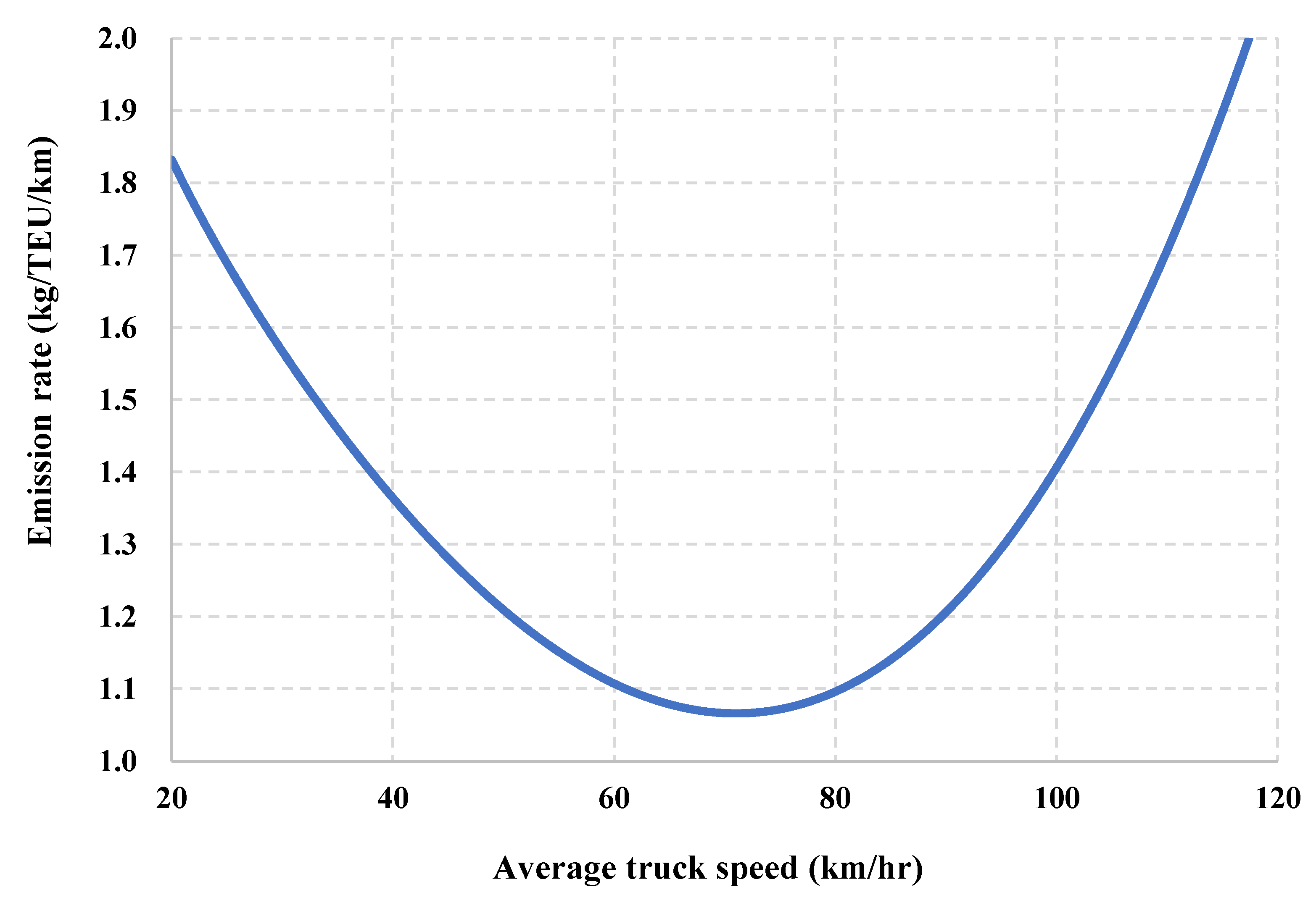
e r o a d p v p = 1576 17.6 · v p + 0.00117 · v p 3 + 36,067 v p 2 · 1.43 0.916 v p · 10 3
where v p > 0 is the truck speed in km/hr in the time range p . Equation (1) is a U-shaped function whose curve is shown in Figure 3. The value of e r o a d p reaches the minimum when v p = 71.02 km/hr. According to Figure 3, the increase of the truck speed within the speed limit of [20, 70] km/hr decreases the emission rate of road service.
The fuzzy truck speed leads to the fuzziness of the speed-dependent rate of CO2 emissions of roads. When the road service yields fuzzy truck speed v 1 p ,   v 2 p ,   v 3 p ,   v 4 p in time range p , the prominent points of its corresponding fuzzy emission rate are based on fuzzy arithmetic operations as in Equation (2):
e ~ r o a d p = e r o a d p v 4 p ,   e r o a d p v 3 p ,   e r o a d p v 2 p ,   e r o a d p v 1 p
The activity-based method [62] is then used to calculate the emissions of the two transportation modes. In this method, the activity intensity of a transportation service is obtained by multiplying its travel distance and the volume of containers it carries. Emissions are then estimated by multiplying the activity intensity and the emission rate of the transportation service.

Modeling of the Fuzziness of the Transfer Process from Road to Rail

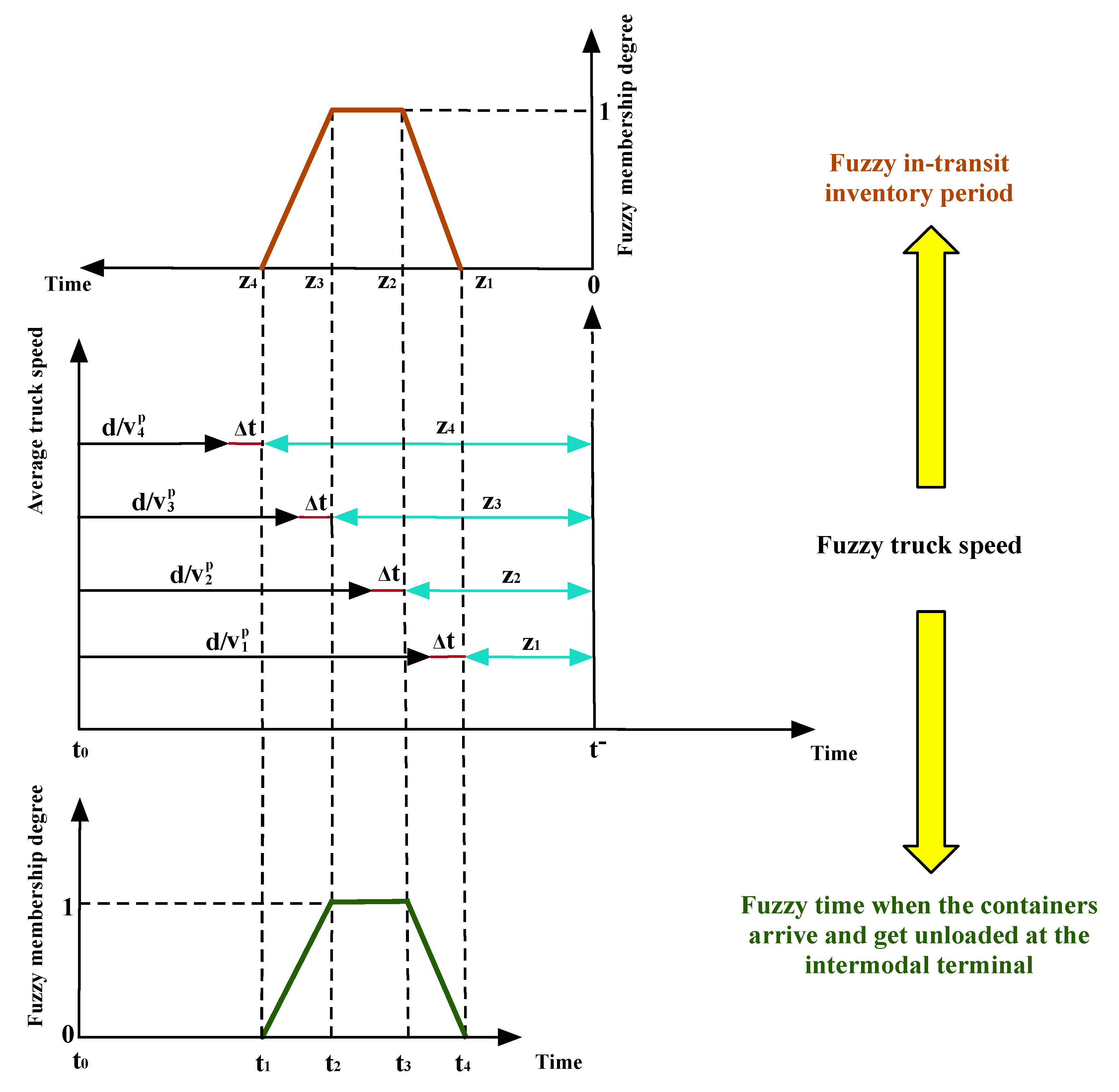
Furthermore, the fuzzy truck speed results in the fuzzy travel time of road service and makes the fuzziness of the time when the containers arrive and get unloaded at the intermodal terminal. As shown in Figure 4, the in-transit inventory period in the transfer from road to rail is also fuzzy when a fixed loading operation start time is regulated by the timetable of rail service.
In Figure 4, t 0 is the truck departure time, d is the travel distance, Δ t is the unloading time of road service, t is the lower bound of the fixed loading operation time window of the train, t 1 ,   t 2 ,   t 3 ,   t 4 shows the time when the containers arrive at the intermodal terminal and get unloaded, and z 1 ,   z 2 ,   z 3 ,   z 4 is the fuzzy in-transit inventory period. As illustrated by Figure 4, when the values of v 1 p , v 2 p , v 3 p , and v 4 p gradually increase in the same degree, the values of z 1 , z 2 , z 3 , and z 4 decrease to 0 successively, and when t = t 1 , the fuzzy in-transit inventory period is 0 ,   0 ,   0 ,   0 [37]. To capture such a variation, the maximum function can be used to model the prominent points of the fuzzy in-transit inventory period [37], i.e., z 1,2 , 3,4 = max t t 4,3 , 2,1 ,   0 . Additionally, if there is an inventory period denoted by π that is free of charge, fuzzy charged in-transit inventory period m 1 ,   m 2 ,   m 3 ,   m 4 can be determined by m 1,2 , 3,4 = max z 1,2 , 3,4 π ,   0 . The successive arrival, unloading, in-transit inventory, and loading operations determine the time when the transfer from road to rail is accomplished.

Modeling of the Soft Delivery Time Window in a Fuzzy Environment

Finally, the fuzzy truck speed leads to the delivery accomplishment time fuzziness. For a certain transportation order, suppose the delivery for its containers is accomplished at t d 1 ,   t d 2 ,   t d 3 ,   t d 4 and its soft delivery time window is b ,   b + . It is possible that t d 1 ,   t d 2 ,   t d 3 ,   t d 4 violates the lower bound, upper bound, or even the two bounds (e.g., t d 1 < b and t d 4 > b + ). Moreover, there are also cases where t d 1 ,   t d 2 ,   t d 3 ,   t d 4 satisfies the two bounds (e.g., t d 1 b and t d 4 b + ). Consequently, there are three situations regarding the lower bound of the soft delivery time window [36]:
(1)
When t d 4 < b , it is definite that the entire fuzzy delivery accomplishment time violates the lower bound of the time window, and the resulting fuzzy time window violation can be represented by b t d 4 ,   b t d 3 , b t d 2 , b t d 1 .
(2)
When t d 1 > b , the fuzzy delivery accomplishment time satisfies the lower bound, and the fuzzy time window violation is 0 ,   0 ,   0 ,   0 .
(3)
When the fuzzy delivery accomplishment time is between the above two situations (i.e., t d 1 b and t d 4 b ), part of the fuzzy delivery accomplishment time violates the lower bound, and the corresponding fuzzy time window violation can be formulated as η ~ = max b t d 4 ,   0 , max b t d 3 ,   0 , max b t d 2 , 0 , max b t d 1 ,   0 , which also includes the first two situations.
Similarly, the violation of the upper bound of the soft delivery time window can be expressed by μ ~ = max t d 1 b + ,   0 , max t d 2 b + ,   0 , max t d 3 b + , 0 , max t d 4 b + ,   0 .
Since there are situations where the lower and upper bounds of the time window are both violated or satisfied, the fuzzy time window violation of the soft delivery time window that is penalized and added into the objective function can be generally formulated as η ~ + μ ~ to integrate all the situations mentioned above.
However, the pickup start time is planned by the intermodal operator and thus a deterministic variable. Therefore, the soft pickup time window is in a deterministic environment. When the pickup of containers starts at w and the soft pickup time window is a ,   a + , violation δ of w concerning a ,   a + is deterministic and can be formulated by the traditional piecewise linear function: δ = a w if w < a ; δ = w a + if w > a + ; and δ = 0 if a w a + .

3.3. Problem Formulation

Above all, in this study, we consider a carbon-efficient RRIRP. The objective of the problem is to minimize the total costs for accomplishing all transportation orders that consist of transportation costs, carbon emission costs, and penalty costs regarding the soft pickup and delivery time windows. Therefore, the objective reflects an integration of economy, carbon efficiency, and timeliness of transportation.
Considering the time flexibility of the road and its time-dependent truck speed, we formulate a truck departure time and speed matching problem taking the following objectives into account:
(1)
Enhancing the transfer efficiency between road and rail by reducing the in-transit inventory.
(2)
Lowering the CO2 emissions of road services selected for transportation orders to improve the carbon efficiency of the road sector.
(3)
Improving the timeliness of transportation by minimizing the time window violation of both pickup and delivery services.
(4)
Ensuring the smooth transfer from road to rail in a fuzzy environment to achieve reliable transportation.
The truck departure time and speed matching problem has the same optimization objectives as the RRIRP. Therefore, we model the RRIRP as a combination of the transportation path planning problem and the truck departure time and speed matching problem. The transportation path planning problem is a foundational decision of the RRIRP. It refers to selecting transportation services to connect the origins and destinations of the transportation orders. The truck departure time and speed matching problem is an extension of transportation path planning and aims to optimize the operations of road services on the planned paths. The two subproblems can be synchronously optimized in the RRIRP to balance the economy, carbon efficiency, timeliness, and reliability of transportation. Finally, we aim to achieve the optimum routing decision with the best comprehensive level on the above goals to meet customer demands.

4. Fuzzy Nonlinear Optimization Model

A fuzzy mixed integer nonlinear programming model is established for the proposed RRIRP. The sets, indices, parameters, and variables in the optimization model are defined in Table 1.

4.1. Optimization Objective

M i n i m i z e k K   ( i , j ) A   s Π i j   ( c rail 1 + c rail 2 d i j s ) q k x i j s k + k K ( i , j ) A ( i τ k j τ k + ) s Γ i j c r o a d 1 d i j s q k x i j s k + ( i , j ) A ( i = τ k j = τ k + ) s Γ i j c r o a d 2 d i j s q k x i j s k + k K i N h N i r S h i c r q k x h i r k + j N i + s S i j c s q k x i j s k + c store k K ( i , j ) A s Π i j m ~ i j s k q k + s Γ i j ϑ i j s k q k + c emission k K ( i , j ) A s Π i j e i j s q k d i j s x i j s k + s Γ i j p P i j s e ~ i j s p q k d i j s u i j s p k + c penalty k K ( δ k + η ~ k + μ ~ k ) q k
Equation (3) is the objective function that minimizes the total costs of accomplishing all transportation orders. In this equation, the first item refers to the travel costs of rail services. The second item calculates the travel costs of road services that implement pickups, deliveries, and truck-only transportation. The combination of the first two items is the travel costs of the RRIRP (denoted by F 1 ).
The third item means the loading/unloading operation costs in the RRIRP used to accomplish the pickup, delivery, and truck-only transportation services and transfer between road and rail (denoted by F 2 ).
The fourth item represents the in-transit inventory costs in the RRIRP caused by the containers’ waiting for the loading operation in the transfer between road and rail at intermodal terminals (denoted by F ~ 3 ). F 1 + F 2 + F ~ 3 calculates the transportation costs for accomplishing transportation activities.
The fifth item shows the CO2 emission costs under the carbon tax policy in the RRIRP (denoted by F ~ 4 ). In this item, the emission rate of a road service in a time range (i.e., e ~ i j s p ) is a fuzzy parameter since the truck speed of the road service is considered fuzzy. Based on the MEET and fuzzy arithmetic operations, e ~ i j s p is determined by Equations (4) and (5).
e i j s p θ = 1576 17.6 · v i j s p 5 θ + 0.00117 · v i j s p 5 θ 3 + 36067 v i j s p 5 θ 2 · 1.43 0.916 v i j s p 5 θ · 10 3 i ,   j A s Γ i j p P i j s θ 1 ,   2 ,   3 ,   4
e ~ i j s p = e i j s p 1 ,   e i j s p 2 ,   e i j s p 3 ,   e i j s p 4 i ,   j A s Γ i j p P i j s

4.2. Constraint Set

h N i s S h i x h i r k j N i + s S i j x i j s k = 1 i = τ k 0 i N \ τ k ,   τ k + 1 i = τ k + k K
Equation (6) is the container flow equilibrium constraint. It ensures that for each transportation order, only the outbound container flow exists at its origin node, and its destination node only has the inbound container flow. This equation also balances the inbound and outbound container flows at intermodal terminals that conduct transfer between road and rail.
s S i j x i j s k 1 k K i ,   j A
Equation (7) ensures that each transportation order is unsplittable during the movement by transportation services on the arcs.
δ k = a k w k ,     i f   w k < a k 0 ,     i f   a k w k a k + w k a k + ,     i f   w k > a k + k K
As a piecewise linear function, Equation (8) calculates the violation of the pickup start time of each transportation order regarding the soft pickup time window.
g τ k k = w k k K
Equation (9) assumes that the planned start time of loading containers of each transportation order on trucks at the origin node equals the transportation order’s pickup start time.
g i k h N i r Π h i l i s + q k · t i r · x h i r k k K i N τ k + \ τ k
Equation (10) ensures that loading containers of each transportation order on trucks at an intermodal terminal should be started after or immediately at the time when the containers get unloaded from the rail service.
p P i j s u i j s p k = x i j s k k K i ,   j A s S i j
Equation (11) regulates the relationship between the transportation service selection variable and the time range selection variable. It means that when a road service is selected to move the containers of a transportation order, a time range should first be determined to plan its truck departure time before moving containers.
n i j s k = f l o o r g i k + q k · t i s + 24 24 k K i ,   j A s Γ i j
Equation (12) uses the floor function, which is a staircase function, to determine the day when the trucks of a road service carrying the containers of a transportation order depart from the predecessor node of an arc.
g i k + q k · t i s 24 · n i j s k 1 o i j s p + ξ · u i j s p k 1 k K i ,   j A s Γ i j p P i j s
g i k + q k · t i s 24 · n i j s k 1 < o i j s p + + ξ · 1 u i j s p k k K i ,   j A s Γ i j p P i j s
Equations (13) and (14) convert the truck departure time into the corresponding clock time (i.e., a time ranging from 0 to 24 by its left-hand formula) and ensures that the converted truck departure time of a road service moving the containers of a transportation order should fall into the selected time range.
g h k + q k · t i r + p P i j s d h i r v h i r p 5 θ · u h i r p k + q k · t i r y i k θ · x h i r k = 0 k K h ,   i A r Γ h i θ 1 ,   2 ,   3 ,   4
y ~ j k = y i k 1 , y i k 2 ,   y i k 3 , y i k 4 k K i N τ k + τ k +
Equation (15) calculates the prominent points of the trapezoidal fuzzy time when the containers of a transportation order arrive at a node and get unloaded from trucks. Equation (16) shows the representation of the trapezoidal fuzzy time.
z i j s k θ max l i s y i k 5 θ ,   0 · x i j s k = 0 k K i ,   j A s Π i j θ 1 ,   2 ,   3 ,   4
z ~ i j s k = z i j s k 1 , z i j s k 2 ,   z i j s k 3 , z i j s k 4 k K i ,   j A s Π i j
Equation (17) calculates the four prominent points of the trapezoidal fuzzy in-transit inventory period of the containers of a transportation order in the transfer from road to rail. Equation (18) shows the representation of this trapezoidal fuzzy variable.
m ijsk θ = max z i j s k θ π ,   0 k K i ,   j A s Π i j θ 1 ,   2 ,   3 ,   4
m ~ i j s k = m i j s k 1 , m i j s k 2 ,   m i j s k 3 , m i j s k 4 k K i ,   j A s Π i j
Equations (19) and (20) determine the trapezoidal fuzzy charged in-transit inventory period of the containers of a transportation order in the transfer from road to rail.
ϑ i j s k max g i k h N i r Π h i l i s + q k · t i r · x h i r k π ,   0 · x h i r k = 0 k K i N τ k + \ τ k i ,   j A s Γ i j
ϑ i j s k = 0 k K i τ k i ,   j A s Γ i j
Equation (21) calculates the deterministic charged in-transit inventory period of the containers of a transportation order in the transfer from rail to road. Equation (22) means that there is no in-transit inventory at the origin nodes of transportation orders since the origin nodes are associated with soft pickup time windows and penalty costs.
y ~ i k + z ~ i j s k + q k · t i s l i s + · x i j s k + ξ · 1 x i j s k k K i ,   j A s Π i j
Equation (23) is a fuzzy constraint since it contains fuzzy variables. It indicates a fuzzy event that the transfer of the containers of a transportation order from road to rail should be accomplished no later than the upper bound of its fixed operation time window (i.e., its fixed loading cutoff time).
k K q k · x i j s k ϖ ~ i j s i ,   j A s Π i j
Similar to Equation (23), Equation (24) is also a fuzzy constraint and represents a fuzzy event that all containers loaded on a rail service should not exceed the capacity.
η k θ = max b k y τ k + k 5 θ ,   0 k K θ 1 ,   2 ,   3 ,   4
η ~ k = η k 1 ,   η k 2 ,   η k 3 ,   η k 4 k K
μ k θ = max y τ k + k θ b k + ,   0 k K θ 1 ,   2 ,   3 ,   4
μ ~ k = μ k 1 ,   μ k 2 ,   μ k 3 ,   μ k 4 k K
Equations (25) and (26) give the trapezoidal fuzzy violation of the delivery accomplishment time of a transportation order regarding the lower bound of its soft delivery time window. Similarly, Equations (27) and (28) present the trapezoidal fuzzy violation regarding the upper bound of the transportation order’s soft delivery time window.
x i j s k 0 ,   1 k K i ,   j A s S i j
u i j s p k 0 ,   1 k K i ,   j A s Γ i j p P i j s
w k 0 k K
g i k 0 k K i N τ k +
n i j s k 0   a n d   i n t e g e r k K i ,   j A s Γ i j
ϑ i j s k 0 k K i ,   j A s Γ i j
δ k 0 k K
y i k 4 y i k 3 y i k 2 y i k 1 0 k K i N τ k + τ k +
z i j s k 4 z i j s k 3 z i j s k 2 z i j s k 1 0 k K i ,   j A s Π i j
m i j s k 4 m i j s k 3 m i j s k 2 m i j s k 1 0 k K i ,   j A s Π i j
η k 4 η k 3 η k 2 η k 1 0 k K
μ k 4 μ k 3 μ k 2 μ k 1 0 k K
Equations (29)~(40) are the variable domain constraints.

5. Solution Approach

The optimization model established as Equations (3)~(40) is fuzzy and nonlinear. The fuzziness of the mode makes it unsolvable and further leads to the issue that crisp solutions to the problem are unattainable for the intermodal operator to plan the transportation scheme. Furthermore, the nonlinearity of the model considerably increases its computational complexity [63]. In this case, this study designs a solution approach based on defuzzification and linearization to process the proposed model to obtain an equivalent reformulation that is both crisp and linear. After processing, the problem becomes solvable and the efficiency of finding the optimal solutions to the problem can be simultaneously enhanced.

5.1. Chance-Constrained Programming with General Fuzzy Measure

CCP is the most extensively used approach that handles fuzzy data or linguistic terms in the fuzzy optimization model and can provide decision-makers with the chances of attainment of the fuzzy objective(s) and fuzzy constraint(s) [64]. The first step of the CCP is to select a fuzzy measure. Then, based on the fuzzy measure, this approach uses the expected value operator and the chance-constrained operator to address the fuzzy objective(s) and fuzzy constraint(s) [65].
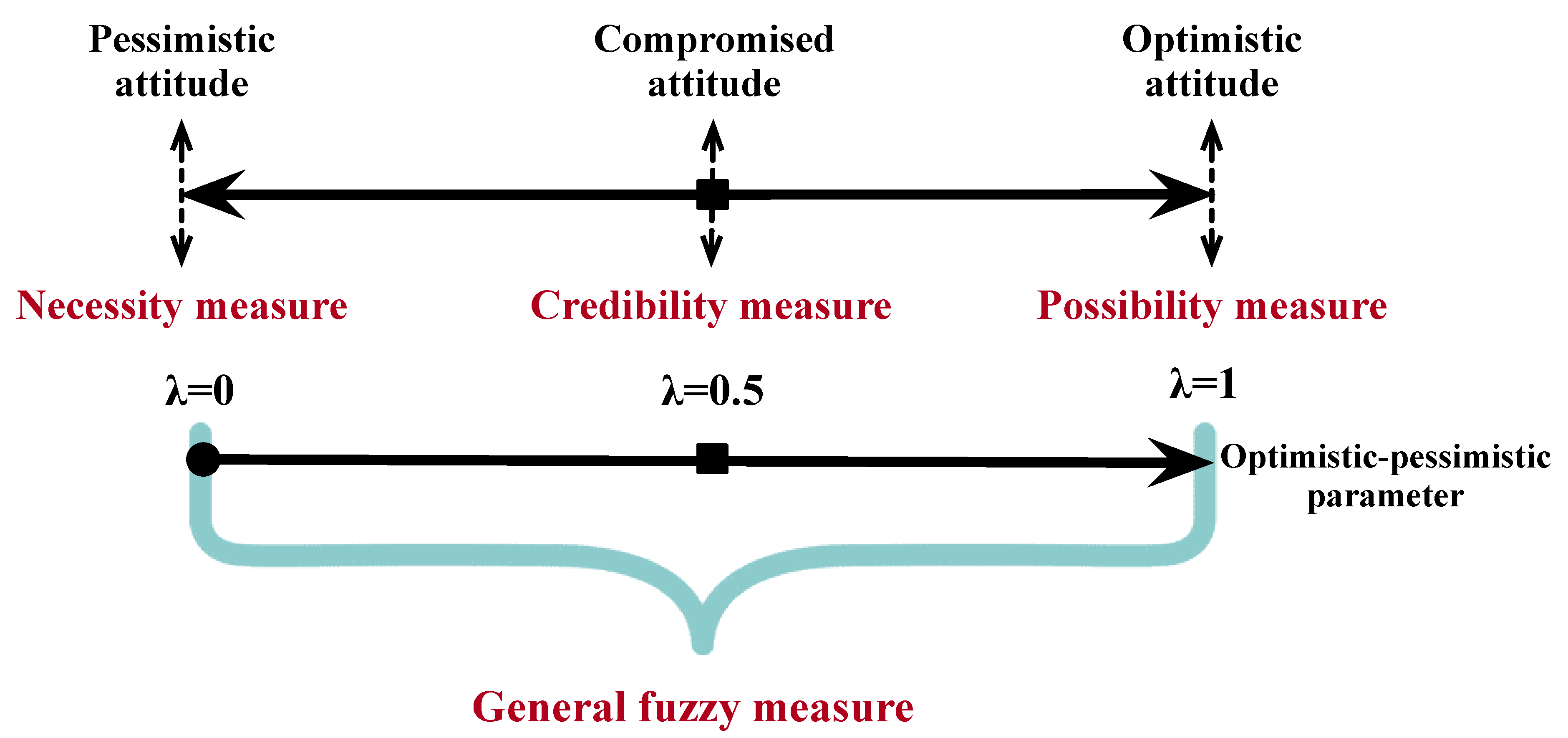
Among the fuzzy measures, possibility and necessity measures are the earliest [66]. Let Θ ,   P Θ ,   P o s denote a possibility space where Θ is a non-empty set and P Θ is the power set of Θ . For a fuzzy event H P Θ , P o s H and N e c H are the possibility and necessity of H , respectively [67], and N e c H = 1 P o s H C , where H C is the complement of H [68]. Possibility and necessity are two extreme measures representing decision-makers’ optimistic and pessimistic viewpoints [69].
However, in practical decision-making, decision-makers’ attitudes usually fluctuate between the two extreme viewpoints. Zhang and Liu [70] propose the credibility measure that is defined by C r H = 0.5 P o s H + N e c H and emphasize that the credibility measure is self-dual compared with possibility and necessity measures: fuzzy event H must hold if C r H = 1 , while it fails if C r H = 0 . Then, Xu and Zhou [69] define general fuzzy measure M e H by Equation (41):
M e H = N e c H + λ P o s H N e c H
where λ 0 ,   1 is the optimistic–pessimistic parameter to determine the combined attitude of a decision-maker.
For general fuzzy measure M e , we have M e H = P o s H when λ = 1 . This case reflects the maximum chance that H holds. We also have M e H = N e c H when λ = 0 . In this case, H holds with minimal chance. When λ = 0 , we obtain M e H = C r H , which expresses the compromised attitudes of decision-makers. Consequently, the fuzzy general measure fully covers the other three measures, which can be seen in Figure 5. It also enables decision-makers to determine the level between optimism and pessimism regarding their preference by modifying the value of λ [71], which makes decision-making more flexible and avoids excessive tendencies to optimistic or pessimistic solutions [72]. As a result, this study adopts the general fuzzy measure to reformulate the fuzzy optimization model of the proposed RRIRP.

5.1.1. Establishing the Expected Objective

Suppose a trapezoidal fuzzy number φ ~ = φ 1 ,   φ 2 ,   φ 3 ,   φ 4 where φ 4 φ 3 φ 2 φ 1 0 . According to Xu and Zhou [69], its expected value is as shown in Equation (42).
E φ ~ = 1 λ 2 φ 1 + φ 2 + λ 2 φ 3 + φ 4
As for the fuzzy objective indicated by Equation (42), its expected value is E F 1 + F 2 + F ~ 3 + F ~ 4 + F ~ 5 . Considering the linearity property of the expected value operator [73], the crisp objective is formulated as Equation (43), where E F ~ 3 , E F ~ 4 , and E F ~ 5 are expressed as Equations (44)–(46), successively. Equation (43) minimizes the expected total costs for accomplishing all transportation orders. The expected objective removes the fuzziness of the initial objective.
M i n i m i z e   F 1 + F 2 + E F ~ 3 + E F ~ 4 + E F ~ 5
E F ~ 3 = c s t o r e · k K i ,   j A s Π i j 1 λ 2 m i j s k 1 + m i j s k 2 + λ 2 m i j s k 3 + m i j s k 4 · q k + s Γ i j ξ i j s k · q k
E F ~ 4 = c e m i s s i o n · k K i ,   j A s Π i j e i j s · q k · d i j s · x i j s k + s Γ i j p P i j s 1 λ 2 e i j s p 1 + e i j s p 2 + λ 2 e i j s p 3 + e i j s p 4 · q k · d i j s · u i j s p k
E F ~ 5 = c p e n a l t y · k K δ k + 1 λ 2 η k 1 + η k 2 + λ 2 η k 3 + η k 4 + 1 λ 2 μ k 1 + μ k 2 + λ 2 μ k 3 + μ k 4 · q k

5.1.2. Establishing the Chance Constraints

Suppose β is a deterministic number and β 0 . Let φ ~ β and φ ~ β represent two fuzzy events. Based on Xu and Zhou [69], the fuzzy general measures of the two events are presented as Equations (47) and (48).
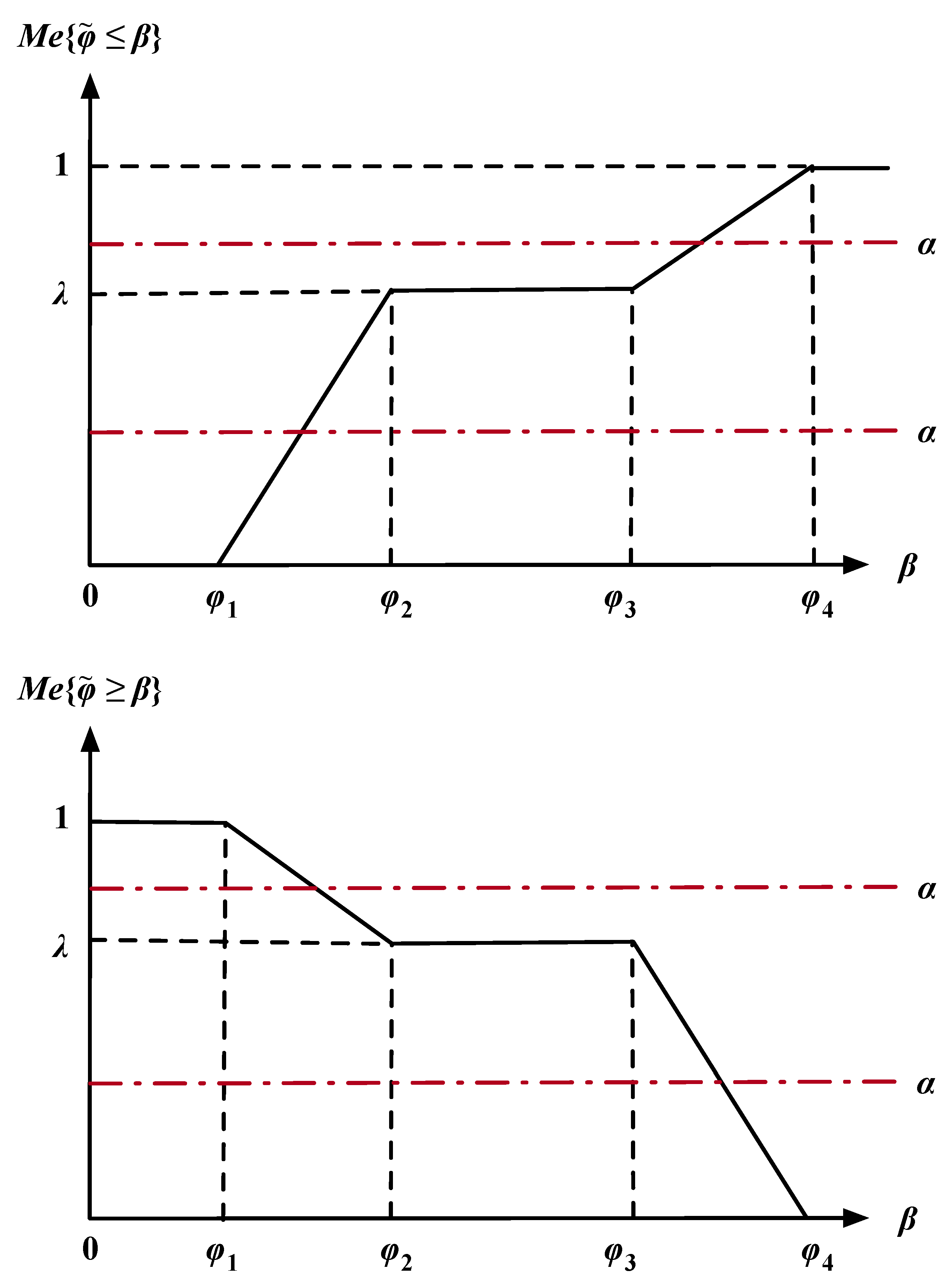
M e φ ~ β = 0 ,     i f   β φ 1 λ β φ 1 φ 2 φ 1 ,     i f   φ 1 β φ 2 λ ,     i f   φ 2 β φ 3 λ + 1 λ β φ 3 φ 4 φ 3 ,     i f   φ 3 β φ 4 1 ,     i f   β φ 4
M e φ ~ β = 1 ,     i f   β φ 1 λ + 1 λ φ 2 β φ 2 φ 1 ,     i f   φ 1 β φ 2 λ ,     i f   φ 2 β φ 3 λ φ 4 β φ 4 φ 3 ,     i f   φ 3 β φ 4 0 ,     i f   β φ 4
The distributions of M e φ ~ β and M e φ ~ β concerning β are illustrated in Figure 6. Figure 6 indicates that M e φ ~ β and M e φ ~ β are both piecewise linear functions concerning β .
Let α 0 ,   1 be the minimum acceptable confidence level that the fuzzy event holds. We have M e φ ~ β α and M e φ ~ β α , which means that the general fuzzy measure of a fuzzy event should be no less than a given confidence level. According to Figure 6, the crisp formulations of M e φ ~ β α and M e φ ~ β α depend on the comparison between the values of λ and α . Using M e φ ~ β α as an example, when α λ , M e φ ~ β α can be rewritten as λ β φ 1 / φ 2 φ 1 α . However, when α > λ , M e φ ~ β α equals to λ + 1 λ β φ 3 / φ 4 φ 3 α . Finally, we can obtain Equation (49) to substitute M e φ ~ β α .
M e φ ~ β α λ α λ φ 1 + α λ φ 2 β ,     i f   α λ 1 α 1 λ φ 3 + α λ 1 λ φ 4 β ,     i f   α > λ
Similarly, we can have Equation (50) to substitute M e φ ~ β α .
M e φ ~ β α α λ φ 3 + λ α λ φ 4 β ,     i f   α λ α λ 1 λ φ 1 + 1 α 1 λ φ 2 β ,     i f   α > λ
Based on the chance-constrained programming that employs the general fuzzy measure, the chance constraint reformulations of the fuzzy constraints, i.e., Equations (23) and (24), are Equations (51) and (52), respectively.
M e y ~ i k + z ~ i j s k + q k · t i s l i s + · x i j s k + ξ · 1 x i j s k α k K i ,   j A s Π i j
M e k K q k · x i j s k ϖ ~ i j s α i ,   j A s Π i j
The above two equations can be further rewritten as Equations (53) and (54) that remove the fuzziness of the initial constraints, respectively. Although realizing the crisp reformulation, the two equations are piecewise and thus nonlinear.
λ α λ y i k 1 + z i j s k 1 + q k · t i s + α λ y i k 2 + z i j s k 2 + q k · t i s l i s + · x i j s k + ξ · 1 x i j s k ,     i f   α λ 1 α 1 λ y i k 3 + z i j s k 3 + q k · t i s + α λ 1 λ y i k 4 + z i j s k 4 + q k · t i s l i s + · x i j s k + ξ · 1 x i j s k ,     i f   α > λ k K i ,   j A s Π i j
α λ ϖ i j s 3 + λ α λ ϖ i j s 4 k K q k · x i j s k ,     i f   α λ α λ 1 λ ϖ i j s 1 + 1 α 1 λ ϖ i j s 2 k K q k · x i j s k ,     i f   α > λ i ,   j A s Π i j
After handling the fuzzy nonlinear optimization model by the CCP, we generate an equivalent crisp reformulation as shown below that eliminates the fuzzy information and is thus solvable.
O b j e c t i v e   f u n c t i o n : E q u a t i o n 43 e x p l a i n e d   b y   E q u a t i o n s 44 ~ 46 C o n s t r a i n t   s e t : E q u a t i o n s 4 , 6 ~ 15 , 17 , 19 , 21 ~ 22 , 25 , 27 , 29 ~ 40 , 53 ~ ( 54 )

5.2. Model Linearization

The CCP model is nonlinear due to the existence of the multiplication of variables and piecewise functions containing variables in various constraints. This study linearizes all the nonlinear constraints as follows to reduce the computational complexity resulting from the nonlinearity of the model and improve the efficiency of problem-solving.
As a piecewise linear function, Equation (8) can be linearized as Equation (55) by adding two non-negative auxiliary variables δ k 1 and δ k 2 that use Equations (56)~(59) to regulate their lower bounds and take the minimization of the two variables with the help of the objective to control their upper bounds.
δ k = δ k 1 + δ k 2 k K
δ k 1 a k w k k K
δ k 2 w k a k + k K
δ k 1 0 k K
δ k 2 0 k K
Proof: 
When w k < a k , the lower bound of the pickup time window is violated. Based on Equation (8), δ k = a k w k . We have δ k 1 a k w k and δ k 2 0 based on Equations (56)~(59). The minimization of δ k resulting from Equation (43) minimizes both δ k 1 and δ k 2 and further leads to that δ k 1 = a k w k and δ k 2 = 0 . Consequently, δ k = δ k 1 + δ k 2 = a k w k . □
When w k > a k + , the upper bound of the pickup time window is violated. Based on Equation (8), δ k = w k a k + . Similarly, we have δ k 1 0 and δ k 2 w k a k + based on Equations (56)~(59). The minimization of both δ k 1 and δ k 2 then results in that δ k 1 = 0 and δ k 2 = w k a k + . Finally, there is δ k = δ k 1 + δ k 2 = w k a k + .
However, when a k w k a k + , the pickup time window is satisfied and δ k = 0 according to Equation (8). We have δ k 1 0 and δ k 2 0 based on Equations (56)~(59) and accordingly have δ k 1 = δ k 2 = 0 and δ k = δ k 1 + δ k 2 = 0 .
Above all, the equivalence of Equations (56)~(59) to Equation (8) is proven.
As a staircase function, Equation (12) can be converted into two inequality constraints as Equations (60) and (61) to regulate the integer variable’s upper and lower bounds. The detailed proof of this linearization can be found in the authors’ previous study [6].
n i j s k g i k + q k · t i s + 24 24 k K i ,   j A s Γ i j
n i j s k > g i k + q k · t i s 24 k K i ,   j A s Γ i j
As a nonlinear equality constraint, Equation (15) equals the two inequality constraints as Equations (61) and (62) based on the linearization method previously designed by the authors [36]. The two linear equations separately regulate the upper and lower bounds of the time when the containers of a transportation order arrive by road and get unloaded at a node.
y j k θ g i k + q k · t i s + p P i j s d i j s v i j s p 5 θ · u i j s p k + q k · t j s + ξ · 1 x i j s k k K i ,   j A s Γ i j θ 1 ,   2 ,   3 ,   4
y j k θ g i k + q k · t i s + p P i j s d i j s v i j s p 5 θ · u i j s p k + q k · t j s + ξ · x i j s k 1 k K i ,   j A s Γ i j θ 1 ,   2 ,   3 ,   4
To linearize Equations (17), (19), (21), (25), and (27), which are the equality constraints associated with the maximum function, we have Equations (64)~(68) together with the domain constraints to regulate the lower bounds of the relevant variables and use the minimization of these variables with the help of the objective to regulate their upper bounds. The detailed proof on the equivalence can be found in the authors’ work [37].
z i j s k θ l i s y i k 5 θ + ξ · x i j s k 1 k K i ,   j A s Π i j θ 1 ,   2 ,   3 ,   4
m ijsk θ z i j s k θ π k K i ,   j A s Π i j θ 1 ,   2 ,   3 ,   4
ϑ i j s k g i k h N i r Π h i l i s + q k · t i r · x h i r k π + ξ · x i j s k 1 k K i N τ k + \ τ k i ,   j A s Γ i j
η k θ b k y τ k + k 5 θ k K θ 1 ,   2 ,   3 ,   4
μ k θ y τ k + k θ b k + k K θ 1 ,   2 ,   3 ,   4
To linearize Equations (53) and (54) that are the piecewise chance constraints, we first define a 0–1 binary variable ϵ : ϵ = 1 means that α > λ ; ϵ = 0 otherwise. ϵ is constrained by Equations (69)~(71) according to its definition. Then, using this auxiliary variable, we can linearize Equation (53) as Equations (72) and (73) and Equation (54) as Equations (74) and (75).
α λ + ξ · ϵ
α > λ ξ · 1 ϵ
ϵ 0 ,   1
λ α λ y i k 1 + z i j s k 1 + q k · t i s + α λ y i k 2 + z i j s k 2 + q k · t i s l i s + · x i j s k + ξ · 1 x i j s k + ξ · ϵ k K i ,   j A s Π i j
1 α 1 λ y i k 3 + z i j s k 3 + q k · t i s + α λ 1 λ y i k 4 + z i j s k 4 + q k · t i s l i s + · x i j s k + ξ · 1 x i j s k + ξ · 1 ϵ k K i ,   j A s Π i j
α λ ϖ i j s 3 + λ α λ ϖ i j s 4 k K q k · x i j s k ξ · ϵ i ,   j A s Π i j
α λ 1 λ ϖ i j s 1 + 1 α 1 λ ϖ i j s 2 k K q k · x i j s k + ξ · ϵ 1 i ,   j A s Π i j
Proof: 
When α > λ , Equation (69) ensures that ϵ is bigger than a sufficient small positive number, while Equation (70) holds under any circumstances. In this case, considering Equation (71), ϵ = 1 , which makes the values of the right-hand formulas of Equations (72) and (74) equal + and , respectively, and ξ · 1 ϵ in Equations (73) and (75) equal 0. Therefore, the solutions to the model are not influenced by Equations (72) and (74) that always hold. In this case, Equations (72)~(75) are equivalent to the parts of Equations (53) and (54) corresponding to α > λ . □
However, when α λ , Equation (69) holds in any case, while Equations (70) and (71) result in that ϵ = 0 . Contrary to the situation where α > λ , ϵ = 0 enables that Equations (73) and (75) always hold, and only Equations (72) and (74), in which ξ · ϵ equals 0, work to influence the solutions to the optimization model. In this case, Equations (72)~(75) are equivalent to the parts of Equations (53) and (54) corresponding to α λ .
Consequently, the equivalence of Equations (53) and (54) to Equations (69)~(75) is proven.
Finally, we obtain an equivalent linear optimization model for the proposed RRIRP whose objective function and constraint set are as shown below. Compared with the nonlinear optimization model, the computational complexity of solving the RRIRP using the linear optimization model has been significantly reduced.
O b j e c t i v e   f u n c t i o n : E q u a t i o n 43 e x p l a i n e d   b y   E q u a t i o n s 44 ~ 46 C o n s t r a i n t   s e t : E q u a t i o n s 4 , 6 ~ 7 , 9 ~ 11 , 13 ~ 14 , 22 , 29 ~ 40 , 55 ~ ( 75 )
Based on the linear optimization model, we can efficiently obtain the optimal solutions to the proposed RRIRP by using mathematical programming software (e.g., LINGO, GAMS, and CPLEX) to implement exact solution algorithms (e.g., branch-and-bound algorithm and simplex algorithm). It should be noted that the linear optimization model is parametric. The values of the optimistic–pessimistic parameter (i.e., λ ) and the confidence level (i.e., α ) in the CCP model should be predetermined by the decision-makers before solving the problem.

6. Empirical Case Study

In this section, we provide an empirical case based on the authors’ previous study [37] to demonstrate the effectiveness of the proposed model and the designed solution algorithm. Furthermore, the case analysis is carried out to draw some conclusions and managerial insights that help the intermodal operator to efficiently organize the RRIT by improving the quality of service and carbon efficiency of the transportation.

6.1. Case Description

In the empirical case, the intermodal operator manages 10 transportation orders whose containers need to be transported from Lanzhou, a northwestern inland city in Gansu Province, China, to Lianyungang, an eastern seaport in Jiangsu Province, China, in the weekly planning horizon. The transportation orders are listed in Table 2. In this table, the time windows of the transportation orders are represented by real numbers by using formula t + 24 · ( n 1 ) to convert clock time t in day n into a real number.
To accomplish the transportation orders, the intermodal operator needs to cooperate with drayage operators, terminal operators, and network operators to construct a RRIT network. Based on Sun et al.’s work [37], a RRIT network shown in Figure S1 in the supplementary file can be used to serve the transportation orders in which there are 12 intermodal terminals handling the transfer between road and rail, 10 rail services (container block trains) that are running periodically, and 13 road services that include 1 conducting the truck-only transportation.
The timetables, emission factors, and fuzzy capacities of the rail services are given in Table S1 in the Supplementary File. All time parameters of the timetables are converted into real numbers using the above formula. The time of a day that a road service arranges the departure time of its trucks is divided into six time ranges: [0:00, 6:00), [6:00, 8:00), [8:00, 10:00), [10:00, 16:00), [16:00, 19:00), and [19:00, 24:00). All road services are subject to this profile. The time-dependent and fuzzy average speeds of the road services and their travel distances are presented in Table S2 in the Supplementary File. Finally, the values of the rest cost/time-related parameters are given in Table 3.
This study uses a ThinkPad Laptop with Intel Core i5-5200U 2.20 GHz CPU and 8 GB RAM to run the mathematical programming software LINGO version 12 to do the computations in which the branch-and-bound algorithm embedded in the software is used to solve the equivalent crisp linear optimization model. The scale of the empirical case is given in Table 4.

6.2. Case Analysis

6.2.1. Sensitivity of the Optimization Results Concerning the Carbon Tax Rate

This section tests the sensitivity of the RRIRP concerning the carbon tax rate to analyze the influence of the carbon tax regulation on the optimization results. We change the carbon tax rate from 10 CNY/t to 100 CNY/t with a step of 10 and present the optimization results under each carbon tax rate in Table 5. The time window violation degree in Table 5 is defined as the multiplication of the time window violation and the demands of containers. It should be noted that 100 CNY/t is the carbon tax rate recommended in the Chinese practice in the year 2030 [74].
In Table 5, the CO2 emissions reflect the carbon efficiency (i.e., environmental objective) of the proposed RRIRP. The time window violation degrees determine its timeliness objective. As we can see from Table 5, when the carbon tax rate varies in an actually feasible range of [0.01, 0.10] CNY/kg, the following conclusions can be drawn:
(1)
The increase of the carbon tax rate leads to a constant rise of the total costs of the RRIRP. However, the travel costs and loading/unloading operation costs of the RRIRP remain unchanged, which clarifies that the transportation paths for the transportation orders are insensitive to the carbon tax rate.
(2)
The increase of the carbon tax rate cannot guarantee lowering the CO2 emissions of the RRIRP. In some cases, increasing the carbon tax rate (e.g., from 0.04 to 0.05 or from 0.06 to 0.07) leads to increased costs and emissions.
(3)
The decrease (increase) of the CO2 emissions increases (decreases) the time window violation degrees. The carbon efficiency and timeliness of the RRIRP cannot reach their respective optimum simultaneously under a feasible carbon tax rate range.
(4)
The change of CO2 emissions concerning the carbon tax rate is caused by the truck departure time and speed matching that makes tradeoffs among lowering costs, reducing emissions, and improving timeliness, which is reflected by the change of the in-transit inventory costs (i.e., E F ~ 3 ) and the time window violation degrees.
Based on the above analysis, we can conclude that the carbon tax regulation is not definitely feasible in all cases in helping the intermodal operator to handle the carbon-efficient RRIRP. Moreover, we find that truck departure time and speed matching plays an essential role in balancing the economy, timeliness, and carbon efficiency of the RRIRP under carbon tax regulation.

6.2.2. Multi-Objective Optimization Analysis Considering the Minimization of Emissions

In the case that λ = 0.8 and α = 0.7 , this study finds that using carbon tax regulation is not feasible for the intermodal operator when its rate falls into a feasible range. Under this situation, the multi-objective optimization that takes the minimization of CO2 emissions as an independent objective can be an alternative for the intermodal operator to balance the economy and carbon efficiency of the RRIRP. In multi-objective optimization, the two objectives are Equations (76) and (77). Then, we adopt the interactive fuzzy programming approach with the bounded objective function [37] to obtain the Pareto solutions to the problem.
Economic   objective :   Ψ 1 = m i n i m i z e   F 1 + F 2 + E F ~ 3 + E F ~ 5
Environmental   objective :   Ψ 2 = m i n i m i z e   E F ~ 4
When taking Ψ 1 as the single objective of the RRIRP, we can obtain Ψ 1 m i n , which is the minimum value of Ψ 1 . Under this situation, the corresponding value of Ψ 2 reaches its maximum value, which is Ψ 2 m a x . On the contrary, when it comes to Ψ 2 as the single objective of the RRIRP, we can find its minimum value Ψ 2 m i n and obtain Ψ 1 ’s maximum value Ψ 1 m a x . Using the above maximum and minimum values of the objectives as the negative ideal solutions and positive ideal solutions, Ψ 1 and Ψ 2 can be converted into Equations (78) and (79) that represent their satisfaction degrees.
μ Ψ 1 = 1 ,   i f   Ψ 1 Ψ 1 m i n Ψ 1 m a x Ψ 1 / Ψ 1 m a x Ψ 1 m i n , i f   Ψ 1 m i n Ψ 1 Ψ 1 m a x 0 , i f   Ψ 1 Ψ 1 m a x
μ Ψ 2 = 1 ,   i f   Ψ 2 Ψ 2 m i n Ψ 2 m a x Ψ 2 / Ψ 2 m a x Ψ 2 m i n , i f   Ψ 2 m i n Ψ 2 Ψ 2 m a x 0 , i f   Ψ 2 Ψ 2 m a x
Employing the bounded objective function to convert μ Ψ 2 into a constraint that the satisfaction degree of the carbon efficiency of the RRIRP should not be lower than a given bound denoted by that falls into the range of [0, 1], we can build the interactive fuzzy programming model. The objective of the model is Equation (80) explained by Equations (44)~(46), and its constraint set includes Equations (4), (6)~(7), (9)~(11), (13)~(14), (22), (29)~(40), (55)~(75), and (81).
M a x i m i z e   μ Ψ 1
μ Ψ 2
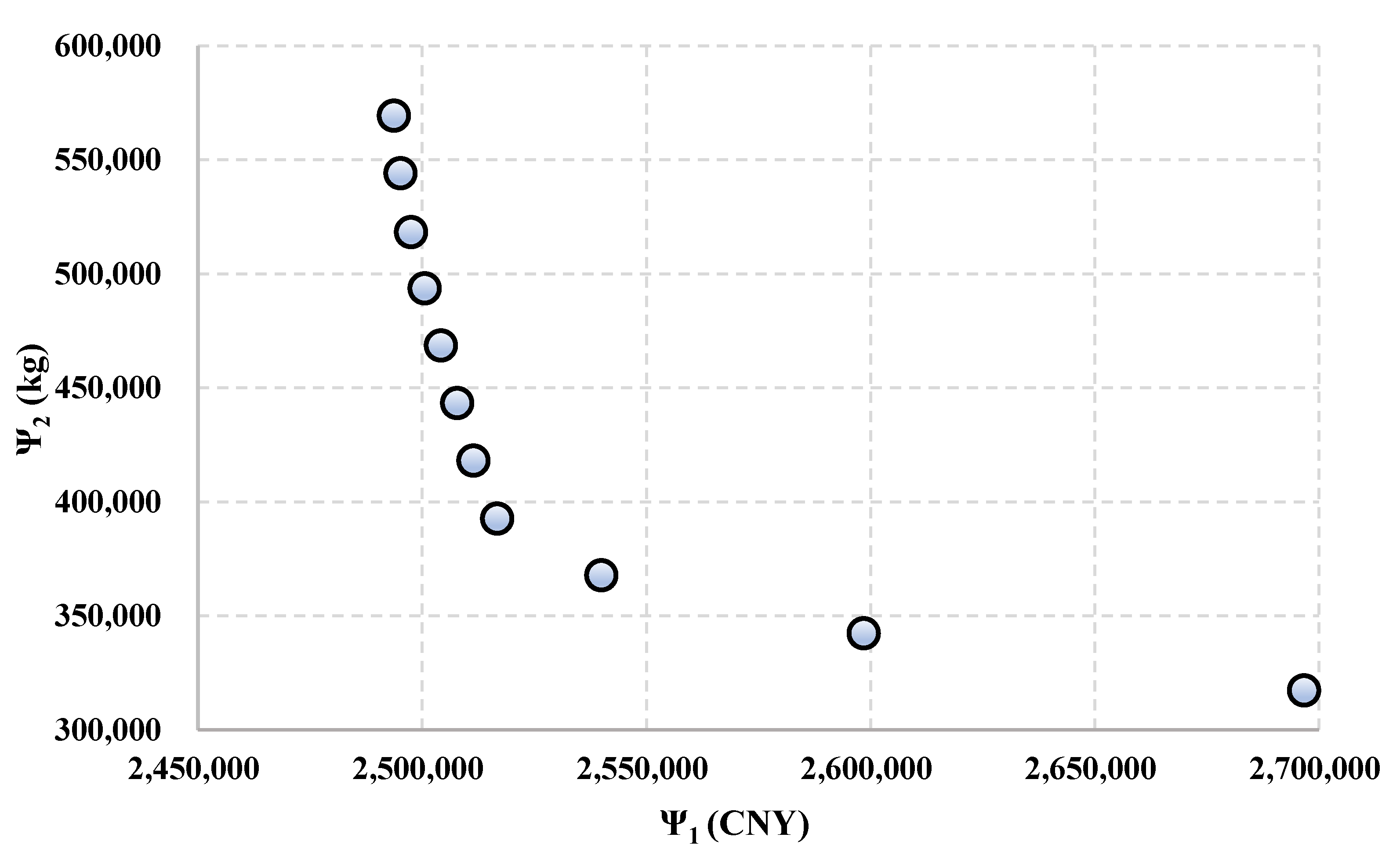
The Pareto solutions to the multi-objective RRIRP can be obtained by modifying the value of from 0 to 1.0 with a step of 0.1 and solving the interactive fuzzy programming model under different values of . The results are shown in Figure 7.
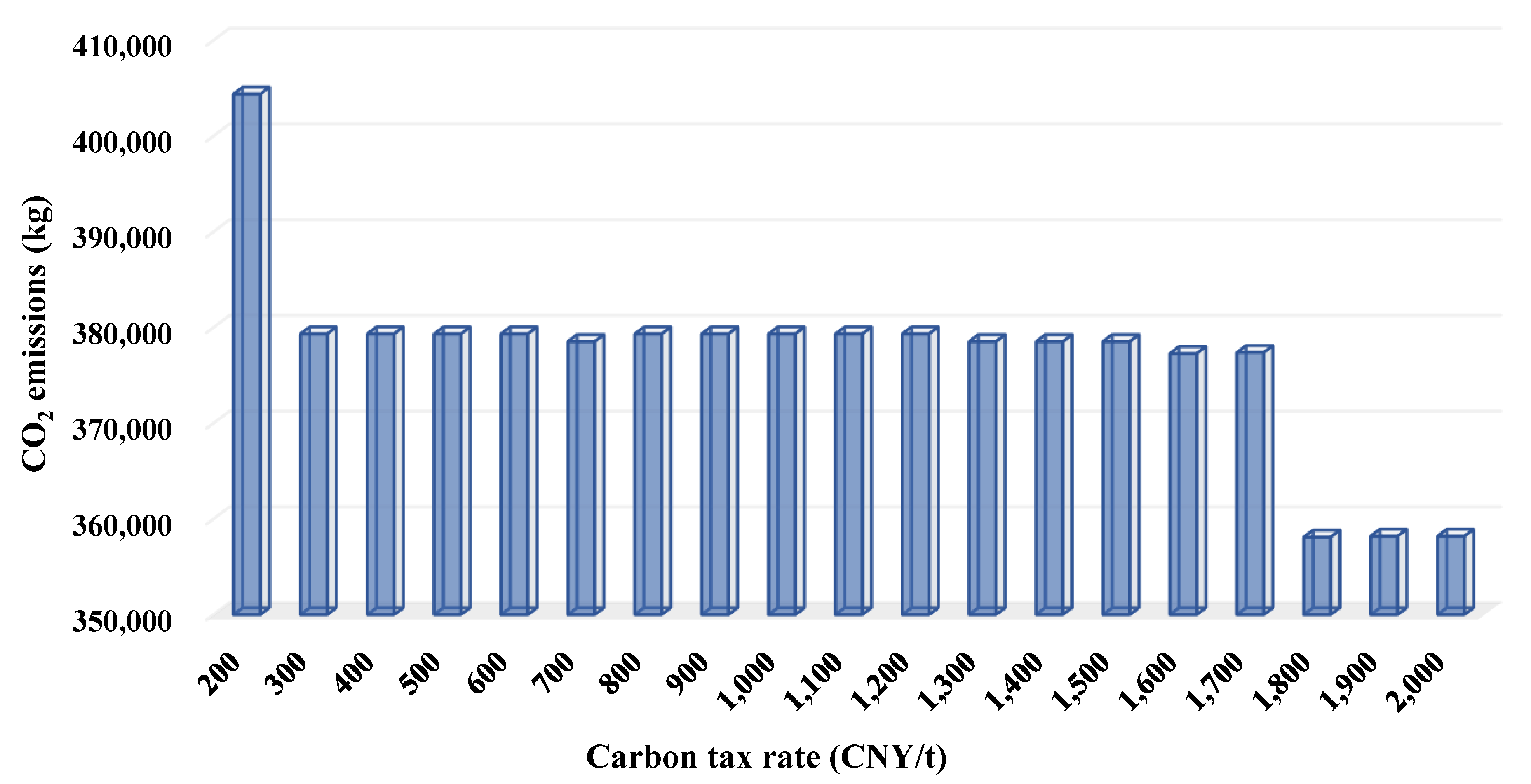
Figure 7 reveals that the economic and environmental objectives are in conflict with each other, and they cannot reach their respective optimum simultaneously. Improving one objective worsens the other. By comparing Table 5 and Figure 7, we find that the carbon tax regulation only finds a considerably limited portion of the emission range covered by the Pareto solutions to the problem. Under this situation, the carbon tax rate should be extensively raised as shown in Figure 8, so that the carbon tax regulation can achieve a similar emission reduction performance to the multi-objective optimization. However, even though the carbon tax rate has been raised to 2000 CNY/t, which is two times higher than the Swedish carbon tax rate (the highest one in the world), the optimization of the RRIRP under carbon tax regulation cannot reach up to the results of the multi-objective optimization.
As a result, the multi-objective optimization is more effective than the carbon tax regulation when balancing the economy and carbon efficiency of the RRIRP. The intermodal operator can select a suitable solution based on the Pareto solutions and customers’ preferences to organize the RRIT for the transportation orders. However, carbon tax regulation can also be used to obtain Pareto solutions in which the carbon tax rate can be treated as the weight assigned to environmental objective Ψ 2 . In this case, the carbon tax regulation is more like the weighted sum method for multi-objective optimization. Moreover, the Pareto solution Ψ 1 ,   Ψ 2 shown in Figure 7 can be easily converted to the solution whose values are Ψ 1 + Ψ 2 · t a x   r a t e   m a d e   b y   t h e   g o v e r n m e n t in case the carbon tax is required by the government and must be paid.
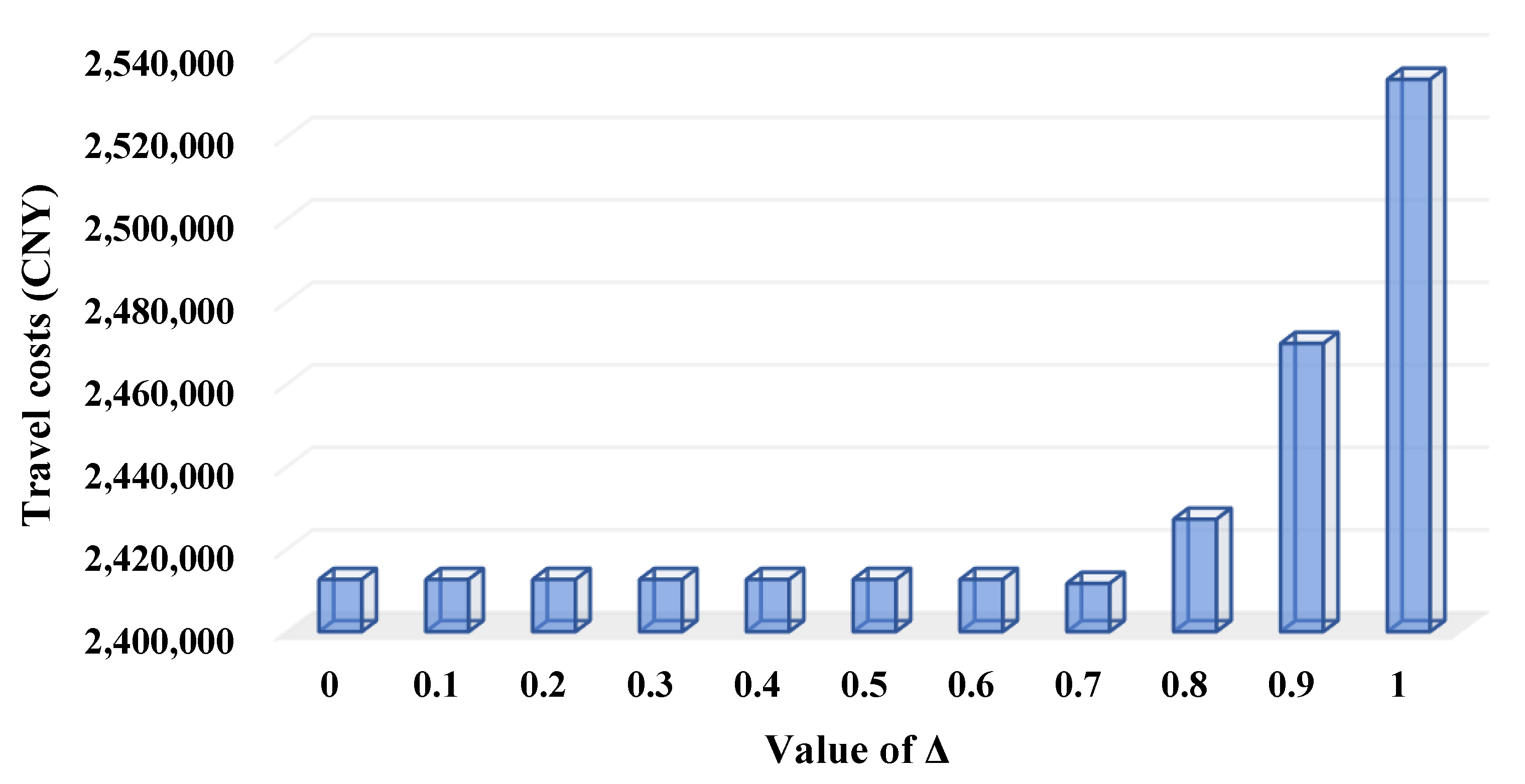
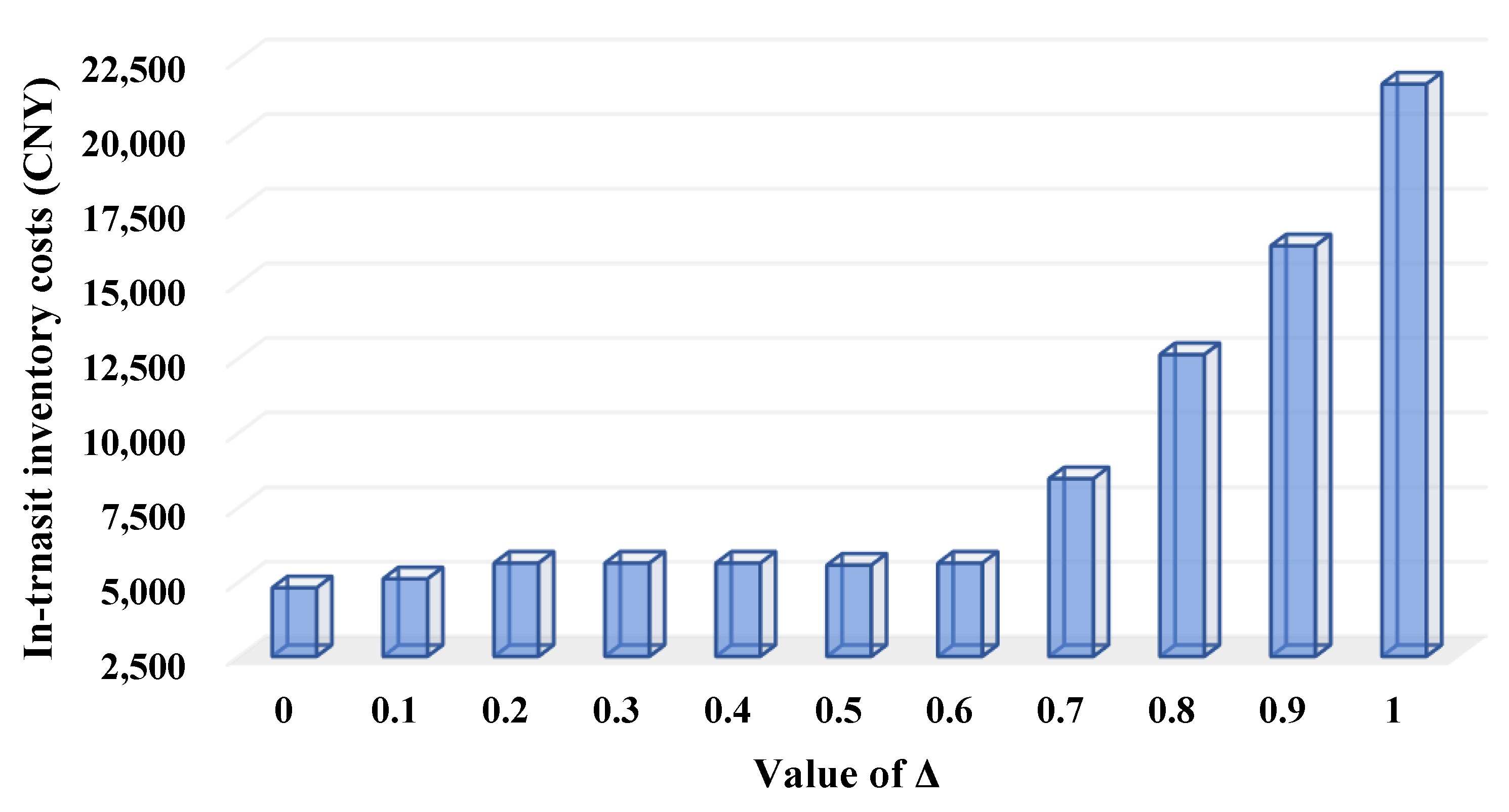
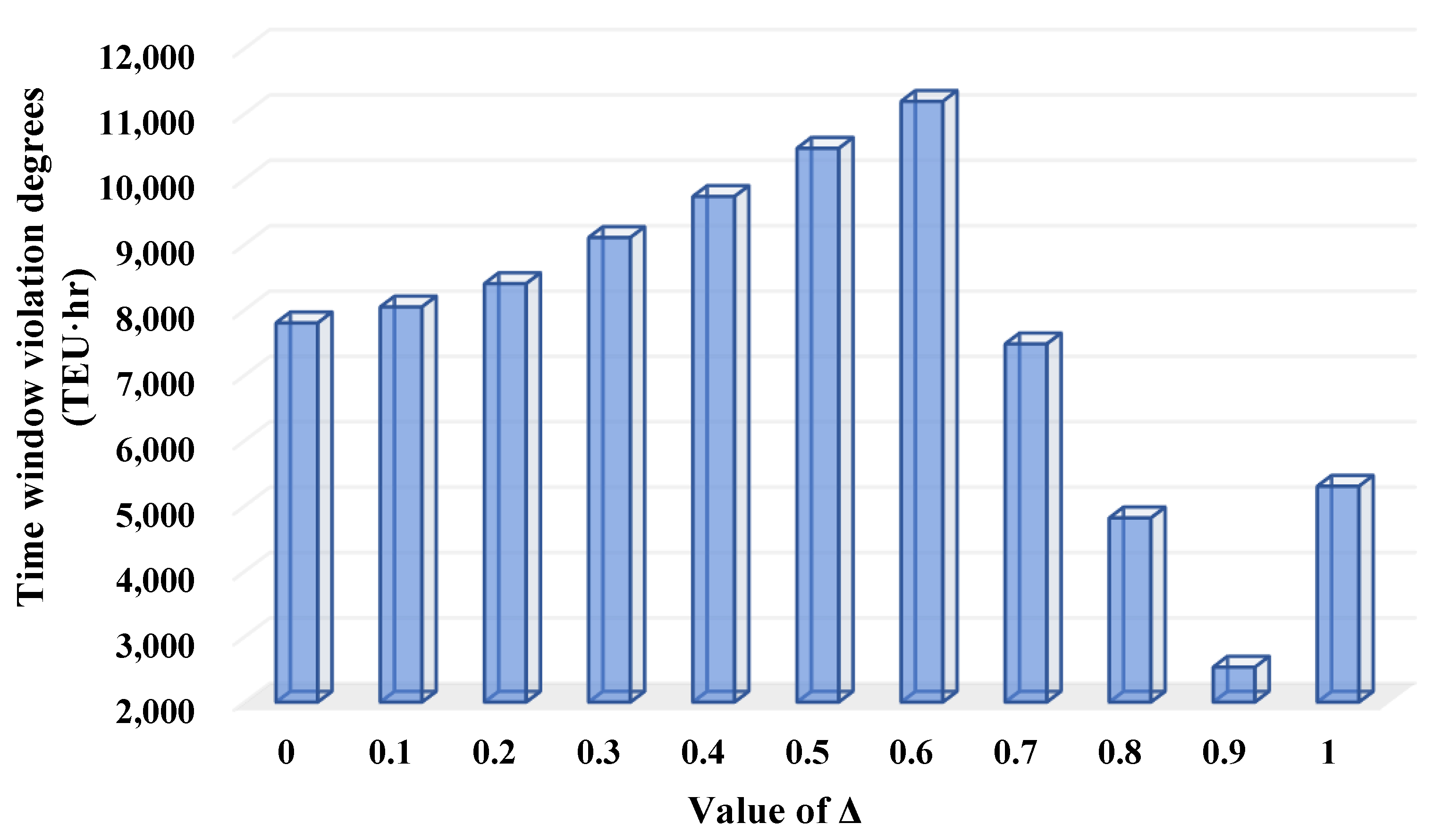
In the multi-objective optimization, the variations of the travel costs, in-transit inventory costs, and the time window violation degrees of the Pareto solutions concerning are illustrated in Figure 9, Figure 10 and Figure 11. Based on Figure 9, Figure 10 and Figure 11, we can summarize the following conclusions:
(1)
When the satisfaction degrees of the environmental objective are low (i.e., 0 0.6 ), the transportation path planning does not contribute to the emission reduction resulting from the increase of since the unchanged travel costs (see Figure 9) of the RRIRP indicates the transportation paths remain unchanged during the emission reduction. In this case, reducing the CO2 emissions depends on the truck departure time and speed matching reflected by the changing in-transit inventory costs and time window violation degrees (see Figure 10 and Figure 11). The truck departure time and speed matching contributes to reducing CO2 emissions by 25.56% when compared with the maximum emissions that are 569,546 kg.
(2)
In the cases where there are lower satisfaction degrees of the environmental objective, reducing the CO2 emissions makes the time window violations increase (see Figure 11), which means the carbon efficiency and timeliness of the RRIRP are in conflict with each other in this case.
(3)
When the satisfaction degrees of the environmental objective are high (i.e., 0.6 1.0 ), the transportation path planning and truck departure time and speed matching both contribute to the emission reduction, which is reflected by the significant change of travel costs, in-transit inventory costs, and time window violation degrees (see Figure 9, Figure 10 and Figure 11). The combination of transportation path planning and truck departure time and speed matching by RRIRP efficiently decreases CO2 emissions by 44.26% compared with the maximum emissions.
(4)
In the cases where there are higher satisfaction degrees of the environmental objective, the time window violation degrees tend to decrease when the CO2 emissions are reduced, except for the variation of from 0.9 to 1.0 that increases the violations (see Figure 11).
Above all, transportation path planning that lowers travel costs enhances the economic objective of RRIRP when it is the dominant consideration of the intermodal operator and the customers. Under this situation, the truck departure time and speed matching helps to improve the carbon efficiency of the RRIRP by scarifying the timeliness. When the environmental objective is more important than the economic objective in the optimization, it needs both transportation path planning and truck departure time and speed matching to work together to remarkably reduce the CO2 emissions of the RRIRP at the expense of scarifying the economy.

6.2.3. Sensitivity of the Optimization Results Concerning λ and α

In this section, we set the carbon tax rate as 1000 CNY/t, which is considered feasible by the literature to realize green transportation [75,76]. Moreover, we consider optimistic–pessimistic parameter λ = 0.3, 0.4, 0.5, 0.6, and 0.7 to represent the decision-makers’ attitudes tending to optimism and pessimism and compromised attitudes. In the sensitivity analysis, α varies from 0.5 to 1.0 with a step of 0.1. We can obtain the optimization results under each combination of λ and α , which is given in Table S3 in the Supplementary File.
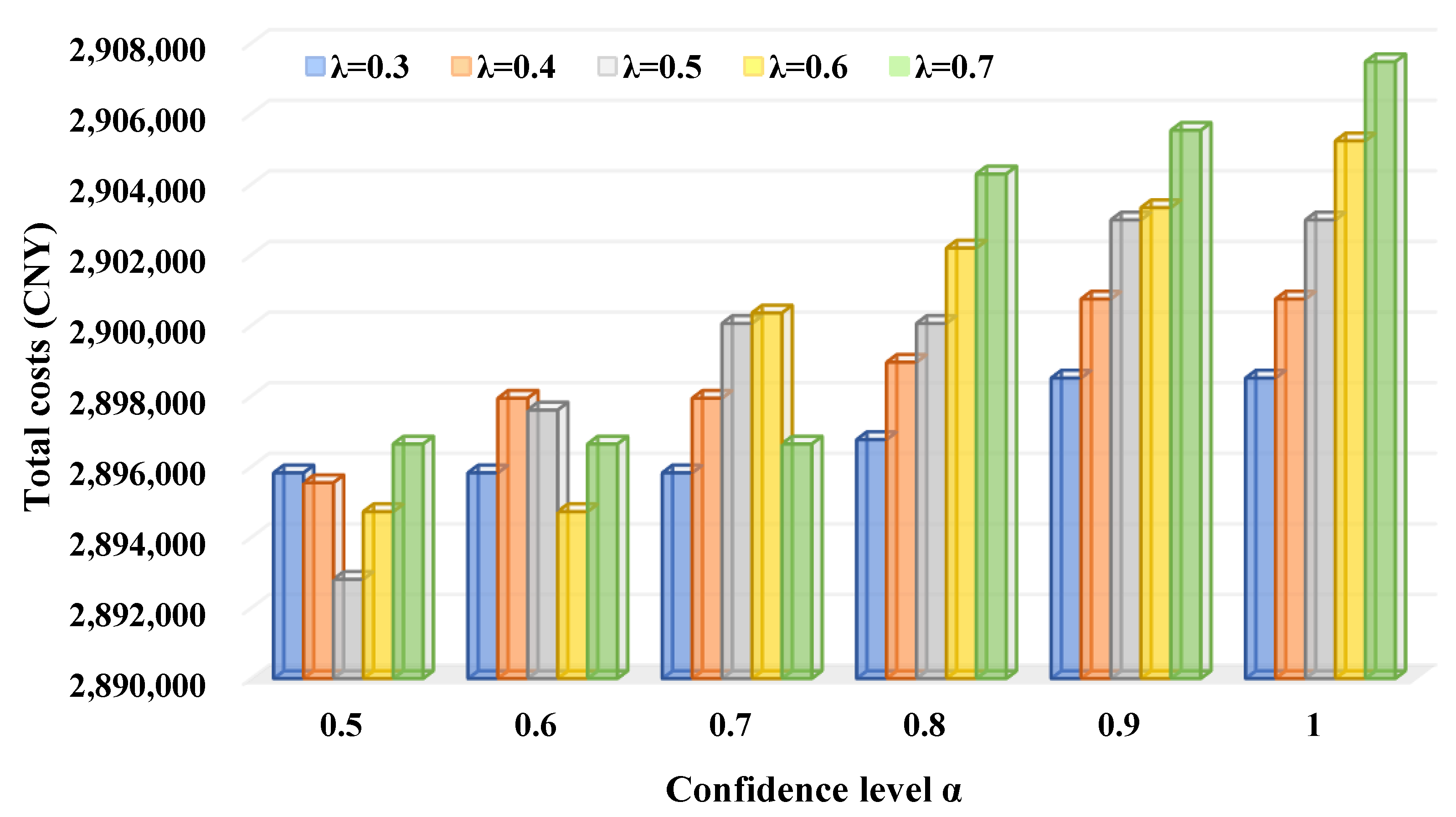
As indicated by Table S3, different solutions to the RRIRP are obtained for different values of the optimistic–pessimistic parameter λ and confidence level α . Therefore, the r RRIRP is sensitive to λ and α . Figure 12 shows the variation of the total costs concerning λ and α and helps to summarize the following conclusions:
(1)
For each value of λ , the increase of α leads to higher total costs that are a combinational reflection of transportation costs, carbon efficiency, and timeliness of the RRIRP since increasing α compresses the feasible solution space of the RRIRP and worsens the solutions found in a smaller space.
(2)
Confidence level α reflects the reliability that the optimization results of the RRIRP are applicable in the actual transportation by selecting the rail services with sufficient capacities and arranging a smooth transfer from road to rail for the transportation orders. Figure 12 demonstrates that the reliability of the RRIRP is conflicting with its total costs. Customers should pay more total costs to the intermodal operator for their transportation orders if they are very cautious on the capacity constraint and fixed operation time window constraint and prefer reliable transportation,
(3)
With the increase of λ , the sensitivity of the total costs of the RRIRP concerning α becomes more significant. Especially, if the customers hold cautious attitudes on the constraints and prefer a higher confidence level to ensure reliable transportation of their containers (i.e., α 0.6 ), the increase of λ raises the total costs when λ < α .
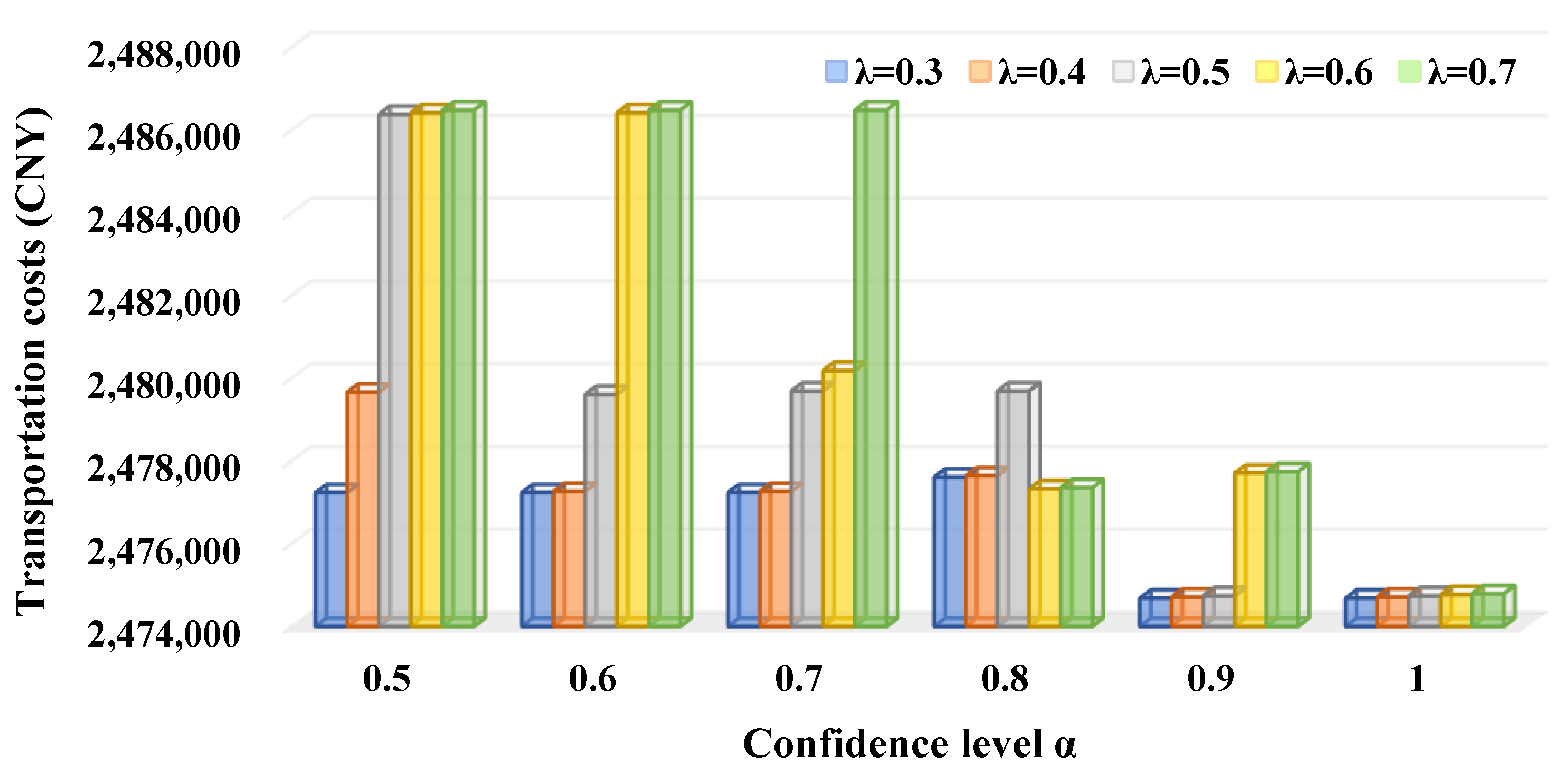
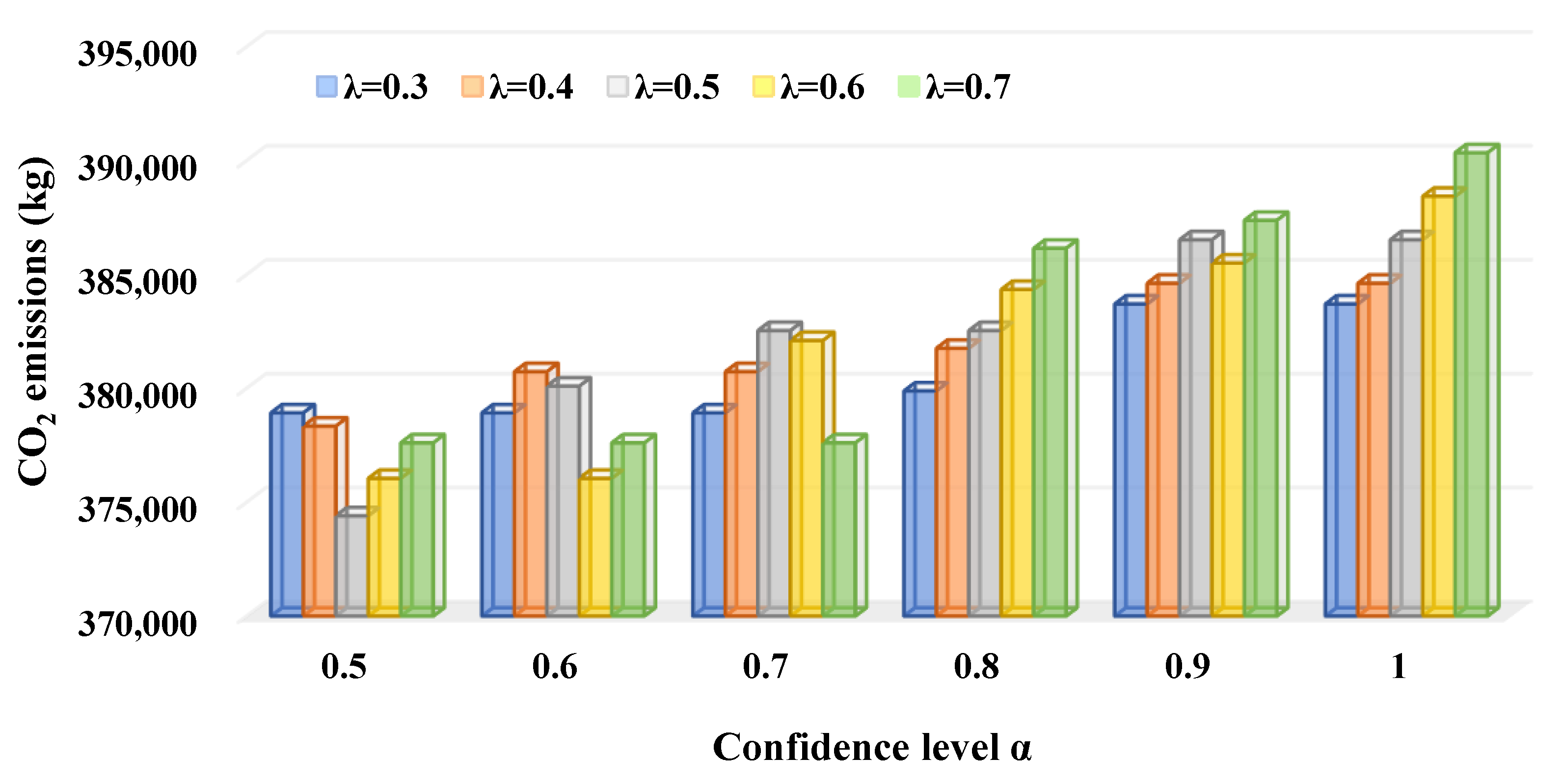
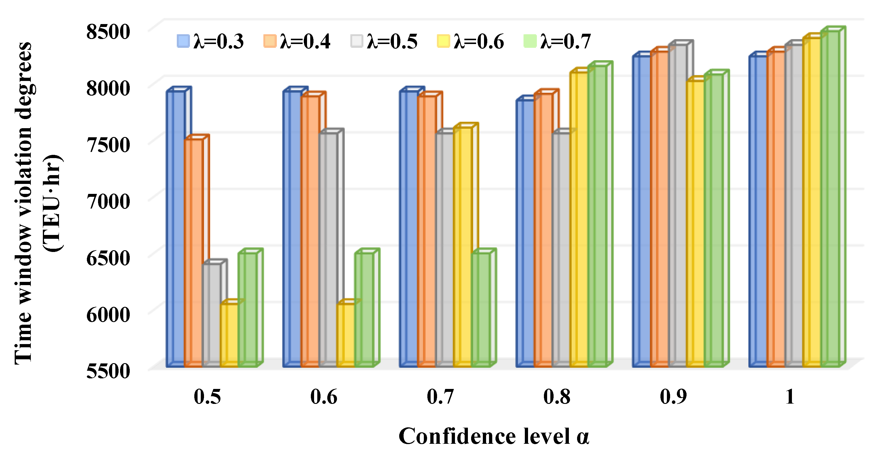
Moreover, we use Figure 13, Figure 14 and Figure 15 to illustrate the sensitivity of the transportation costs, CO2 emissions (carbon efficiency), and time window violation degrees (timeliness) in the total costs concerning λ and α .
Based on the sensitivity shown in Figure 13, Figure 14 and Figure 15, the three components that formulate the total costs of the RRIRP are sensitive to   α and λ . Figure 13, Figure 14 and Figure 15 indicate the following:
(1)
With the increase of α , the transportation costs of the RRIRP tend to decrease. However, the CO2 emissions and the time window violation degrees tend to increase. The increase of the carbon tax and penalty costs are more significant than the decrease of the transportation costs, which leads to the increase of the total costs illustrated by Figure 12.
(2)
The optimization of the RRIRP balances the three components included in the total costs that are treated as the RRIRP objective. As α increases to improve reliability, transportation costs are saved at the expense of scarifying the carbon efficiency and timeliness of the RRIRP. In this case, improving the economy and reliability of the RRIRP worsens its timeliness and carbon efficiency.
(3)
The change of λ fluctuates the transportation costs, CO2 emissions, and time window violation degrees of the RRIRP. As λ increases, it is more sensitive to α .
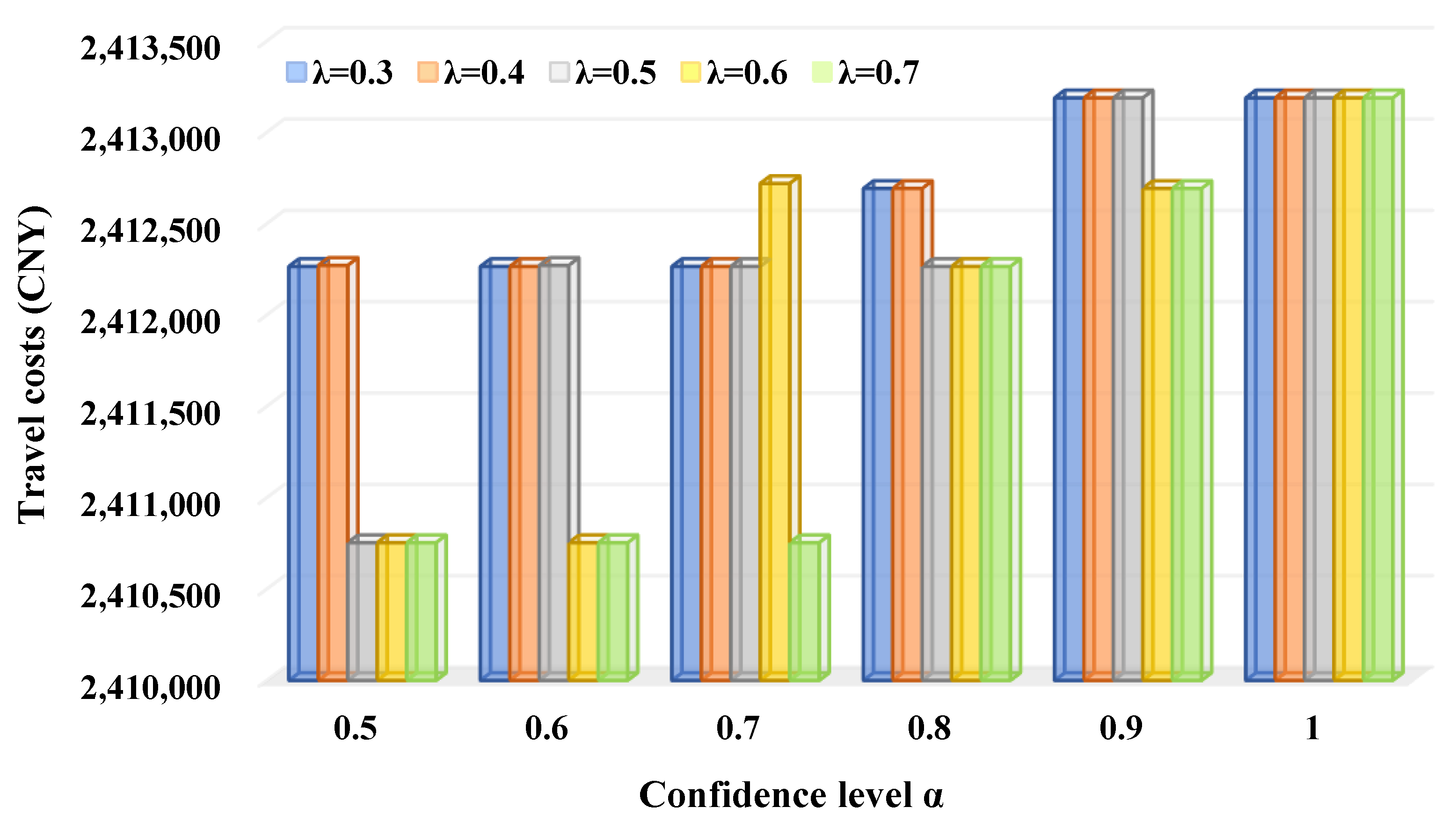
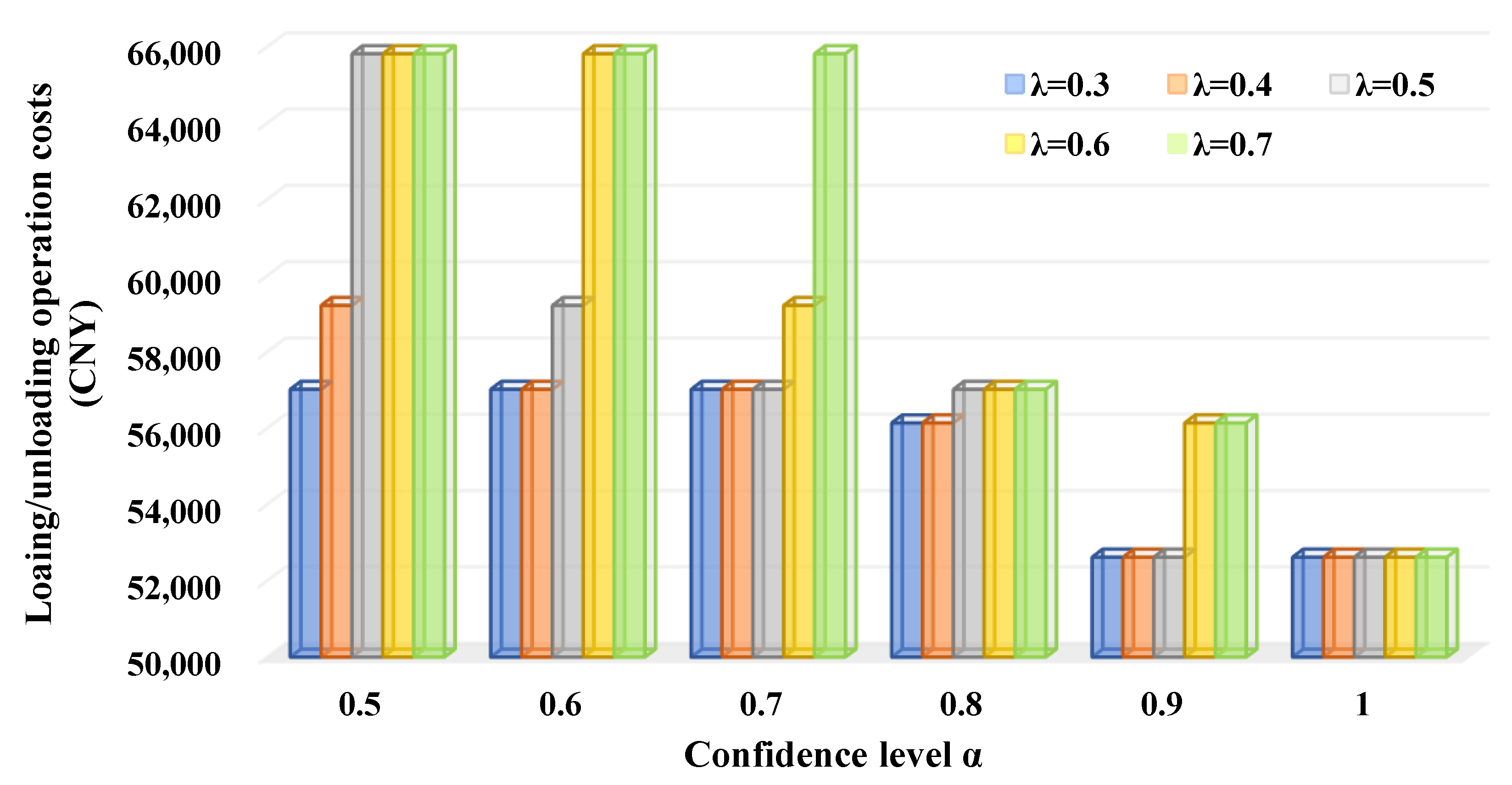
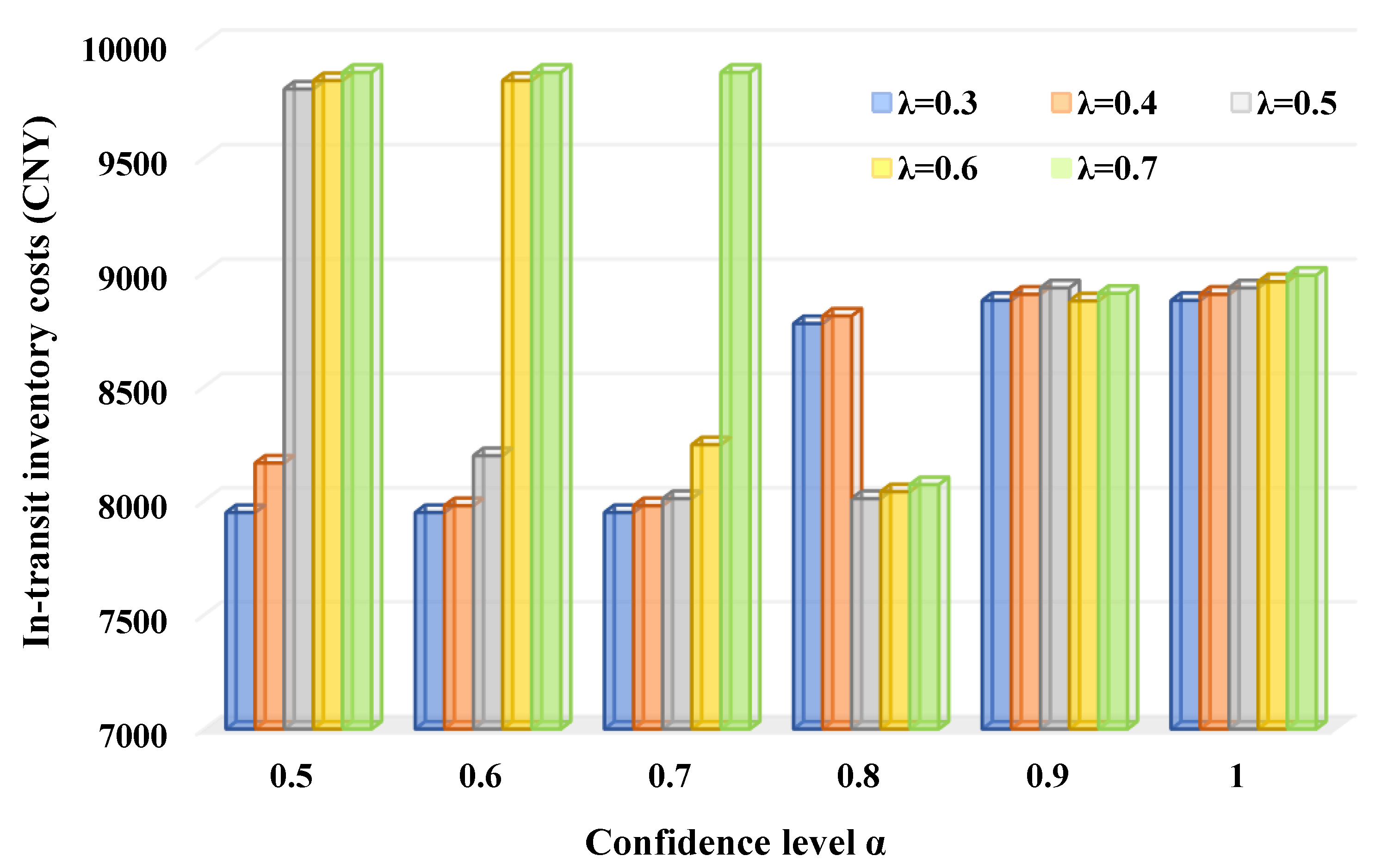
To reveal the performance of transportation path planning and truck departure time and speed matching in sensitivity, we also give the variations of travel costs, loading/unloading operation costs, and in-transit inventory concerning λ and α , which are illustrated in Figure 16, Figure 17 and Figure 18.
As we can see from Figure 16, Figure 17 and Figure 18, the three components that formulate the transportation costs of the RRIRP are sensitive to λ and α . The above sensitivity indicates the following:
(1)
The increase of α results in the change of the travel costs, loading/unloading operation costs, and in-transit inventory costs, which shows that the transportation path is modified and the rematch of truck departure times and speeds occurs.
(2)
With the increase of α , the decrease of the loading/unloading operation costs proves that more transportation orders are accomplished by truck-only transportation where the intermodal transfer that causes loading/unloading operation costs does not exist.
(3)
Although saving loading/unloading operation costs, the use of truck-only transportation tends to increase travel costs (see Figure 16) and make the transportation of containers emit more CO2 (see Figure 14).
(4)
However, truck-only transportation can avoid the risk associated with the fuzzy constraints that the capacities are insufficient and disrupt the intermodal transfer. Therefore, truck-only transportation enhances the reliability of the RRIRP and is realized by transportation path planning. Consequently, the RRIT system established in our study (see Figure 1) is more reliable than the hub-and-spoke system.
(5)
When high confidence levels are needed (i.e., α 0.8 ), the increasing use of truck-only transportation should reduce the in-transit inventory costs that only exist in the intermodal transfer. However, as indicated by Figure 18, the in-transit inventory costs still increase, which means that truck departure times and speeds are rematched to enable an early arrival of trucks at the intermodal terminals to ensure that the transfer from road to rail can be accomplished smoothly.
However, in the above sensitivity analysis, we cannot identify regular changes in the transportation costs (including travel costs, loading/unloading operation costs, and in-transit inventory costs), CO2 emissions, and time window violation degrees concerning λ . Furthermore, it is difficult to determine which value of λ is the best for RRIRP since it refers to the optimistic–pessimistic attitudes of decision-makers (intermodal operator and customers) that are subjective and might be changed in different decision-making conditions.
In summary, the proposed model can effectively incorporate the decision-makers’ optimistic–pessimistic attitudes and confidence levels into the RRIRP in a fuzzy environment and present solutions that can fully express the two degrees. If the decision-makers yield optimistic (pessimistic) attitudes on the problem, they can set a bigger (smaller) value of the optimistic–pessimistic parameter λ . A higher confidence level α can be employed if the decision-makers hold cautious attitudes on the constraints. As indicated by Table S3, by using the proposed model, the decision-makers can obtain the best solution that satisfies their requirements on the objective and constraints to organize the RRIT to accomplish the transportation orders, which shows the advantages of the proposed model.

7. Conclusions

In this study, we present a carbon-efficient RRIRP with soft time windows and truck departure time and speed matching in a time-dependent and fuzzy environment. The proposed RRIRP is formulated as a combination of a transportation path planning problem and a truck departure time and speed matching problem. Therefore, under carbon tax regulation, reducing CO2 emissions is driven by the synchronous optimization of the two subproblems in the optimization problem. The truck speed fuzziness and rail capacity fuzziness are simultaneously modeled in the proposed RRIRP to improve the reliability of capacity assignment and intermodal transfer arrangement in the RRIRP to provide customers with reliable transportation in which the induced fuzziness of emission rates of roads, the transfer from road to rail, and the violation of the soft delivery time windows are comprehensively modeled. Based on the above considerations, this study proposes a CCP model with general fuzzy measure to deal with the proposed RRIRP.
From the empirical case study, we can draw the following conclusions that can help the intermodal operator to organize efficient RRIT:
(1)
When the carbon tax rate is in a reasonable range, carbon tax regulation depends on the truck departure time and speed matching to drive the reduction of CO2 emissions. Furthermore, carbon tax regulation depends on a relatively high tax rate to realize the emission reduction of the RRIRP, which might cause its infeasibility in some cases.
(2)
Multi-objective optimization provides an effective option for the intermodal operator to balance the economy and carbon efficiency of the RRIRP. It also reveals that lowering the transportation and penalty costs are conflicting with reducing CO2 emissions. The intermodal operator can make effective tradeoffs between them using the Pareto solutions.
(3)
Transportation path planning dominates the RRIRP when improving carbon efficiency is paid less attention, in which transportation services with lower travel costs are selected to form the transportation paths. However, a significant improvement in carbon efficiency resulting from the requirement for environmental protection requires cooperation between transportation path planning and truck departure time and speed matching.
(4)
Customers’ attitudes toward the objective and constraints considerably influence the RRIRP. Especially when customers are cautious about the constraints and prefer reliable transportation, they need to pay more costs for their transportation orders. In this case, the cost objective that combines transportation costs, CO2 emissions, and violation of soft time windows reaches a balanced state where transportation costs are saved at the expense of scarifying the carbon efficiency and timeliness of the RRIRP.
(5)
The RRIT system indicated by Figure 1 is more reliable than the hub-and-spoke system and should be attached to great importance in practical transportation. Both transportation path planning that motivates the use of truck-only transportation and truck departure time and speed matching that ensures the early arrival of trucks at intermodal terminals contribute to improving the reliability of the RRIRP.
(6)
Using the proposed CCP model, the intermodal operator can always find an optimum solution as the transportation scheme to organize the RRIT to meet the customers’ preferences and accomplish the transportation orders with the best service.
In this study, the hub congestion in the hub-and-spoke network is not considered by the problem model when formulating the transfer between road and rail in the intermodal terminals. Hub congestion causes the queuing of the containers and also leads to the uncertainty of loading and unloading operations, which influences the efficiency and reliability of the transfer process in the intermodality. Therefore, in our future study, we will model the congestion of the intermodal terminals that serve as hubs in the road–rail intermodal routing problem. A queuing system under uncertainty may be established and integrated into the routing.
The current study discusses the effect of the optimistic–pessimistic parameter and confidence level on the optimization results of the CCP model based on general fuzzy measures using sensitivity analysis. Although the two interactive parameters are determined by decision-makers subjectively, our future work would like to study if there are methods that can help decision-makers efficiently select the suitable values of the parameters during the routing decision-making.
Last but not least, we will design a heuristic algorithm to solve the large-scale problem considering the hardness of its NP. The challenge of the algorithm design for the proposed problem is how to represent the solutions with both 0–1 binary and non-negative continuous variables, generating feasible initial solutions and updating them. If a heuristic algorithm can be developed, its accuracy and efficiency can be verified by comparing it with the exact solution approach proposed in this study.

Supplementary Materials

The following supporting information can be downloaded at https://www.mdpi.com/article/10.3390/systems11080403/s1. Figure S1: Distribution of origin, destination, and intermodal terminals in the road–rail intermodal transportation network. Table S1: Rail services for long-haul transportation in the empirical case. Table S2: Road services for pickups, deliveries, and truck-only transportation in the empirical case. Table S3: Sensitivity of the optimization results concerning λ and α.

Author Contributions

Conceptualization: Y.S., G.S. and B.H.; data curation: Y.S.; formal analysis: Y.S., G.S., B.H. and J.G.; funding acquisition: Y.S.; investigation: Y.S., G.S., B.H. and J.G.; methodology: Y.S., G.S., B.H. and J.G.; resources: Y.S. and G.S.; software: Y.S. and G.S.; supervision: Y.S.; validation: Y.S., B.H. and J.G.; writing—original draft: Y.S., G.S. and J.G.; writing—review and editing: Y.S. and B.H. All authors have read and agreed to the published version of the manuscript.

Funding

This study was funded by the Shandong Provincial Natural Science Foundation of China under Grant Nos. ZR2023MG020 and ZR2021MG053 and the University-Industry Collaborative Education Program of the Ministry of Education of China under Grant No. 220601369102256.

Data Availability Statement

All data generated or analyzed during this study are included in this paper and its Supplementary File.

Conflicts of Interest

The authors declare no conflict of interest.

References

  1. Lu, Q.; Chai, J.; Wang, S.; Zhang, Z.G.; Sun, X.C. Potential energy conservation and CO2 emissions reduction related to China’s road transportation. J. Clean. Prod. 2020, 245, 118892. [Google Scholar] [CrossRef]
  2. Feng, Y.; Ning, M.; Lei, Y.; Sun, Y.; Liu, W.; Wang, J. Defending blue sky in China: Effectiveness of the “Air Pollution Prevention and Control Action Plan” on air quality improvements from 2013 to 2017. J. Environ. Manag. 2019, 252, 109603. [Google Scholar] [CrossRef] [PubMed]
  3. Tong, H.; Peng, J.; Zhang, Y.; Fang, T.; Zhang, J.; Men, Z.; Liu, Y.; Wu, L.; Wang, T.; Ren, F.; et al. Environmental benefit analysis of “road-to-rail” policy in China based on a railway tunnel measurement. J. Clean. Prod. 2021, 316, 128227. [Google Scholar]
  4. Tamannaei, M.; Zarei, H.; Rasti-Barzoki, M. A game theoretic approach to sustainable freight transportation: Competition between road and intermodal road-rail systems with government intervention. Transp. Res. Part B Methodol. 2021, 153, 272–295. [Google Scholar] [CrossRef]
  5. Wang, R.; Yang, K.; Yang, L.; Gao, Z. Modeling and optimization of a poport system under uncertain information. Eng. Appl. Artif. Intell. 2018, 72, 423–436. [Google Scholar] [CrossRef]
  6. Sun, Y. A robust possibilistic programming approach for a road-rail intermodal routing problem with multiple time windows and truck operations optimization under carbon cap-and-trade policy and uncertainty. Systems 2022, 10, 156. [Google Scholar] [CrossRef]
  7. Heggen, H.; Molenbruch, Y.; Caris, A.; Braekers, K. Intermodal container routing: Integrating long-haul routing and local drayage decisions. Sustainability 2019, 11, 1634. [Google Scholar] [CrossRef]
  8. Chen, X.; Zuo, T.; Lang, M.; Li, S.; Li, S. Integrated optimization of transfer station selection and train timetables for road-rail intermodal transport network. Comput. Ind. Eng. 2022, 165, 107929. [Google Scholar] [CrossRef]
  9. Zhang, Y.; Guo, W.; Negenborn, R.R.; Atasoy, B. Synchromodal transport planning with flexible services: Mathematical model and heuristic algorithm. Transp. Res. Part C Emerg. Technol. 2022, 140, 103711. [Google Scholar] [CrossRef]
  10. Wang, Y.; Assogba, K.; Fan, J.; Xu, M.; Liu, Y.; Wang, H. Multi-depot green vehicle routing problem with shared transportation resource: Integration of time-dependent speed and piecewise penalty cost. J. Clean. Prod. 2019, 232, 12–29. [Google Scholar] [CrossRef]
  11. Jabali, O.; Van Woensel, T.; De Kok, A.G. Analysis of travel times and CO2 emissions in time-dependent vehicle routing. Prod. Oper. Manag. 2012, 21, 1060–1074. [Google Scholar] [CrossRef]
  12. Nasri, M.I.; Bektaş, T.; Laporte, G. Route and speed optimization for autonomous trucks. Comput. Oper. Res. 2018, 100, 89–101. [Google Scholar] [CrossRef]
  13. Sun, Y.; Li, X.; Liang, X.; Zhang, C. A bi-objective fuzzy credibilistic chance-constrained programming approach for the hazardous materials road-rail multimodal routing problem under uncertainty and sustainability. Sustainability 2019, 11, 2577. [Google Scholar] [CrossRef]
  14. Foroozesh, N.; Karimi, B.; Mousavi, S.M. Green-resilient supply chain network design for perishable products considering route risk and horizontal collaboration under robust interval-valued type-2 fuzzy uncertainty: A case study in food industry. J. Environ. Manag. 2022, 307, 114470. [Google Scholar] [CrossRef]
  15. Fazayeli, S.; Eydi, A.; Kamalabadi, I.N. Location-routing problem in multimodal transportation network with time windows and fuzzy demands: Presenting a two-part genetic algorithm. Comput. Ind. Eng. 2018, 119, 233–246. [Google Scholar] [CrossRef]
  16. Delbart, T.; Molenbruch, Y.; Braekers, K.; Caris, A. Uncertainty in intermodal and synchromodal transport: Review and future research directions. Sustainability 2021, 13, 3980. [Google Scholar] [CrossRef]
  17. Chang, Y.T.; Lee, P.T.W.; Kim, H.J.; Shin, S.H. Optimization model for transportation of container cargoes considering short sea shipping and external cost: South Korean case. Transp. Res. Rec. 2010, 2166, 99–108. [Google Scholar] [CrossRef]
  18. Zhang, J.; Ding, H.W.; Wang, X.Q.; Yin, W.J.; Zhao, T.Z.; Dong, J. Mode choice for the intermodal transportation considering carbon emissions. In Proceedings of the 2011 IEEE International Conference on Service Operations, Logistics and Informatics, Beijing, China, 10–12 July 2011; pp. 297–301. [Google Scholar]
  19. Guo, W.; Atasoy, B.; Beelaerts van Blokland, W.; Negenborn, R.R. A global intermodal shipment matching problem under travel time uncertainty. In Lecture Notes in Computer Science, Proceedings of the Computational Logistics: 11th International Conference, ICCL 2020, Enschede, The Netherlands, 28–30 September 2020; Proceedings 11; Springer International Publishing: Cham, Switzerland, 2020; pp. 553–568. [Google Scholar]
  20. Duan, X.; Heragu, S. Carbon Emission Tax Policy in an Intermodal Transportation Network. In Proceedings of the IIE Annual Conference. Proceedings, Nashville, TN, USA, 30 May–2 June 2015; Institute of Industrial and Systems Engineers (IISE): Peachtree Corners, GA, USA, 2015; p. 566. [Google Scholar]
  21. Zhang, D.; He, R.; Li, S.; Wang, Z. A multimodal logistics service network design with time windows and environmental concerns. PLoS ONE 2017, 12, e0185001. [Google Scholar] [CrossRef]
  22. Cheng, X.Q.; Jin, C.; Wang, C.; Mamatok, Y. Impacts of different low-carbon policies on route decisions in intermodal freight transportation: The case of the west river region in China. In Proceedings of the International Forum on Shipping, Ports and Airports (IFSPA), Hong Kong, China, 20–24 May 2019. [Google Scholar]
  23. Demir, E.; Bektaş, T.; Laporte, G. A comparative analysis of several vehicle emission models for road freight transportation. Transp. Res. Part D Transp. Environ. 2011, 16, 347–357. [Google Scholar] [CrossRef]
  24. Ji, H.; Wu, P. Sailing route and speed optimization for green intermodal transportation. In Proceedings of the 2020 IEEE 5th International Conference on Intelligent Transportation Engineering (ICITE), Beijing, China, 11–13 September 2020; pp. 18–22. [Google Scholar]
  25. Resat, H.G.; Turkay, M. Design and operation of intermodal transportation network in the Marmara region of Turkey. Transp. Res. Part E Logist. Transp. Rev. 2015, 83, 16–33. [Google Scholar] [CrossRef]
  26. Kontovas, C.; Psaraftis, H.N. Reduction of emissions along the maritime intermodal container chain: Operational models and policies. Marit. Policy Manag. 2011, 38, 451–469. [Google Scholar] [CrossRef]
  27. Fan, Q.; Jin, Y.; Wang, W.; Yan, X. A performance-driven multi-algorithm selection strategy for energy consumption optimization of sea-rail intermodal transportation. Swarm Evol. Comput. 2019, 44, 1–17. [Google Scholar] [CrossRef]
  28. Zhang, D.; Wang, X.; Li, S.; Ni, N.; Zhang, Z. Joint optimization of green vehicle scheduling and routing problem with time-varying speeds. PLoS ONE 2018, 13, e0192000. [Google Scholar] [CrossRef]
  29. Qian, J.; Eglese, R. Fuel emissions optimization in vehicle routing problems with time-varying speeds. Eur. J. Oper. Res. 2016, 248, 840–848. [Google Scholar] [CrossRef]
  30. Ehmke, J.F.; Campbell, A.M.; Thomas, B.W. Vehicle routing to minimize time-dependent emissions in urban areas. Eur. J. Oper. Res. 2016, 251, 478–494. [Google Scholar] [CrossRef]
  31. Braekers, K.; Caris, A.; Janssens, G.K. Time-Dependent Routing of Drayage Operations in the Service Area of Intermodal Terminals; DIME Università di Genova: Genova, Italy, 2012. [Google Scholar]
  32. Sun, Y.; Hrušovský, M.; Zhang, C.; Lang, M. A time-dependent fuzzy programming approach for the green multimodal routing problem with rail service capacity uncertainty and road traffic congestion. Complexity 2018, 2018, 8645793. [Google Scholar] [CrossRef]
  33. Guo, W.; Atasoy, B.; van Blokland, W.B.; Negenborn, R.R. A dynamic shipment matching problem in hinterland synchromodal transportation. Decis. Support Syst. 2020, 134, 113289. [Google Scholar]
  34. Teng, W.; Chen, B.Y.; Lam, W.H.; Gong, W.; Shi, C.; Tam, M.L. Bi-objective reliable eco-routing considering uncertainties of travel time and fuel consumption. Transp. B Transp. Dyn. 2023, 11, 1071–1091. [Google Scholar] [CrossRef]
  35. Sandamali, G.G.N.; Su, R.; Zhang, Y. Flight routing and scheduling under departure and en route speed uncertainty. IEEE Trans. Intell. Transp. Syst. 2019, 21, 1915–1928. [Google Scholar]
  36. Sun, Y. Fuzzy approaches and simulation-based reliability modeling to solve a road-rail intermodal routing problem with soft delivery time windows when demand and capacity are uncertain. Int. J. Fuzzy Syst. 2020, 22, 2119–2148. [Google Scholar] [CrossRef]
  37. Sun, Y.; Yu, N.; Huang, B. Green road-rail intermodal routing problem with improved pickup and delivery services integrating truck departure time planning under uncertainty: An interactive fuzzy programming approach. Complex Intell. Syst. 2022, 8, 1459–1486. [Google Scholar] [CrossRef]
  38. Lu, Y.; Lang, M.; Sun, Y.; Li, S. A fuzzy intercontinental road-rail multimodal routing model with time and train capacity uncertainty and fuzzy programming approaches. IEEE Access 2020, 8, 27532–27548. [Google Scholar] [CrossRef]
  39. Uddin, M.; Huynh, N. Reliable routing of road-rail intermodal freight under uncertainty. Netw. Spat. Econ. 2019, 19, 929–952. [Google Scholar] [CrossRef]
  40. Elbert, R.; Müller, J.P.; Rentschler, J. Tactical network planning and design in multimodal transportation–A systematic literature review. Res. Transp. Bus. Manag. 2020, 35, 100462. [Google Scholar] [CrossRef]
  41. Lu, K.; Liao, H.; Zavadskas, E.K. An overview of fuzzy techniques in supply chain management: Bibliometrics, methodologies, applications and future directions. Technol. Econ. Dev. Econ. 2021, 27, 402–458. [Google Scholar] [CrossRef]
  42. Chang, T.S. Best routes selection in international intermodal networks. Comput. Oper. Res. 2008, 35, 2877–2891. [Google Scholar] [CrossRef]
  43. Xiong, G.; Wang, Y. Best routes selection in multimodal networks using multi-objective genetic algorithm. J. Comb. Optim. 2014, 28, 655–673. [Google Scholar] [CrossRef]
  44. Xie, Y.; Lu, W.; Wang, W.; Quadrifoglio, L. A multimodal location and routing model for hazardous materials transportation. J. Hazard. Mater. 2012, 227, 135–141. [Google Scholar] [CrossRef]
  45. Fang, Y.; Jia, X. Hazmat route optimization by road-rail intermodal transport in the silk road economic zone. Sci. Technol. Eng. 2023, 23, 6614–6622. [Google Scholar]
  46. Winebrake, J.J.; Corbett, J.J.; Falzarano, A.; Hawker, J.S.; Korfmacher, K.; Ketha, S.; Zilora, S. Assessing energy, environmental, and economic tradeoffs in intermodal freight transportation. J. Air Waste Manag. Assoc. 2008, 58, 1004–1013. [Google Scholar] [CrossRef]
  47. Zhou, J.M.; Wei, H.X.; Zhao, Y.Z.; Ma, Y.J. China-Europe container multimodal transport path selection based on multi-objective optimization. Mechatron. Intell. Transp. Syst. 2023, 2, 72–88. [Google Scholar] [CrossRef]
  48. Heinold, A.; Meisel, F. Emission oriented vs. time oriented routing in the European intermodal rail/road freight transportation network. Lect. Notes Logist. 2019, 2019, 188–202. [Google Scholar]
  49. Peng, Y.; Xiao, Y.; Zhou, X.; Liu, S. Optimization on the multimodal transport routing problem with time window and timetable. China Sci. Pap. 2021, 16, 211–216. [Google Scholar]
  50. Ayar, B.; Yaman, H. An intermodal multicommodity routing problem with scheduled services. Comput. Optim. Appl. 2012, 53, 131–153. [Google Scholar] [CrossRef]
  51. Moccia, L.; Cordeau, J.F.; Laporte, G.; Ropke, S.; Valentini, M.P. Modeling and solving a multimodal transportation problem with flexible-time and scheduled services. Networks 2011, 57, 53–68. [Google Scholar] [CrossRef]
  52. Sun, Y.; Lang, M. Modeling the multicommodity multimodal routing problem with schedule-based services and carbon dioxide emission costs. Math. Probl. Eng. 2015, 2015, 406218. [Google Scholar] [CrossRef]
  53. Chen, D.; Zhang, Y.; Gao, L.; Thompson, R.G. Optimizing multimodal transportation routes considering container use. Sustainability 2019, 11, 5320. [Google Scholar] [CrossRef]
  54. Boussedjra, M.; Bloch, C.; El Moudni, A. An exact method to find the intermodal shortest path (ISP). In Proceedings of the IEEE International Conference on Networking, Sensing and Control, Taipei, Taiwan, 21–23 March 2004; Volume 2, pp. 1075–1080. [Google Scholar]
  55. Bierwirth, C.; Kirschstein, T.; Meisel, F. On transport service selection in intermodal rail/road distribution networks. Bus. Res. 2012, 5, 198–219. [Google Scholar] [CrossRef]
  56. Janic, M. Modelling the full costs of an intermodal and road freight transport network. Transp. Res. Part D Transp. Environ. 2007, 12, 33–44. [Google Scholar] [CrossRef]
  57. Wang, Q.Z.; Chen, J.M.; Tseng, M.L.; Luan, H.M.; Ali, M.H. Modelling green multimodal transport route performance with witness simulation software. J. Clean. Prod. 2020, 248, 119245. [Google Scholar] [CrossRef]
  58. Li, Z.; Liu, Y.; Yang, Z. An effective kernel search and dynamic programming hybrid heuristic for a multimodal transportation planning problem with order consolidation. Transp. Res. Part E Logist. Transp. Rev. 2021, 152, 102408. [Google Scholar] [CrossRef]
  59. Yang, X.; Low, J.M.; Tang, L.C. Analysis of intermodal freight from China to Indian Ocean: A goal programming approach. J. Transp. Geogr. 2011, 19, 515–527. [Google Scholar] [CrossRef]
  60. Hickman, J.; Hassel, D.; Joumard, R.; Samaras, Z.; Sorenson, S. Methodology for Calculating Transport Emissions and Energy Consumption; The National Academies of Sciences, Engineering, and Medicine: Washington, DA, USA, 1999. [Google Scholar]
  61. Sung, I.; Nielsen, P. Speed optimization algorithm with routing to minimize fuel consumption under time-dependent travel conditions. Prod. Manuf. Res. 2020, 8, 1–19. [Google Scholar] [CrossRef]
  62. Liao, C.H.; Tseng, P.H.; Lu, C.S. Comparing carbon dioxide emissions of trucking and intermodal container transport in Taiwan. Transp. Res. Part D Transp. Environ. 2009, 14, 493–496. [Google Scholar] [CrossRef]
  63. Resat, H.G.; Turkay, M. A discrete-continuous optimization approach for the design and operation of synchromodal transportation networks. Comput. Ind. Eng. 2019, 130, 512–525. [Google Scholar] [CrossRef]
  64. Peykani, P.; Hosseinzadeh Lotfi, F.; Sadjadi, S.J.; Ebrahimnejad, A.; Mohammadi, E. Fuzzy chance-constrained data envelopment analysis: A structured literature review, current trends, and future directions. Fuzzy Optim. Decis. Mak. 2022, 21, 197–261. [Google Scholar] [CrossRef]
  65. Sun, Y.; Liang, X.; Li, X.; Zhang, C. A fuzzy programming method for modeling demand uncertainty in the capacitated road–rail multimodal routing problem with time windows. Symmetry 2019, 11, 91. [Google Scholar] [CrossRef]
  66. Zadeh, L.A. Fuzzy sets as a basis for a theory of possibility. Fuzzy Sets Syst. 1978, 1, 3–28. [Google Scholar] [CrossRef]
  67. Nahmias, S. Fuzzy variables. Fuzzy Sets Syst. 1978, 1, 97–110. [Google Scholar] [CrossRef]
  68. Dubois, D.; Prade, H. Operations on fuzzy numbers. Int. J. Syst. Sci. 1978, 9, 613–626. [Google Scholar] [CrossRef]
  69. Xu, J.; Zhou, X. Approximation based fuzzy multi-objective models with expected objectives and chance constraints: Application to earth-rock work allocation. Inf. Sci. 2013, 238, 75–95. [Google Scholar] [CrossRef]
  70. Zheng, Y.; Liu, B. Fuzzy vehicle routing model with credibility measure and its hybrid intelligent algorithm. Appl. Math. Comput. 2006, 176, 673–683. [Google Scholar] [CrossRef]
  71. Shiri, M.; Ahmadizar, F.; Thiruvady, D.; Farvaresh, H. A sustainable and efficient home health care network design model under uncertainty. Expert Syst. Appl. 2023, 211, 118185. [Google Scholar] [CrossRef]
  72. Roshan, M.; Tavakkoli-Moghaddam, R.; Rahimi, Y. A two-stage approach to agile pharmaceutical supply chain management with product substitutability in crises. Comput. Chem. Eng. 2019, 127, 200–217. [Google Scholar] [CrossRef]
  73. Kundu, P.; Kar, S.; Maiti, M. Multi-objective multi-item solid transportation problem in fuzzy environment. Appl. Math. Model. 2013, 37, 2028–2038. [Google Scholar] [CrossRef]
  74. Wang, J.; Yan, G.; Jiang, K.; Liu, L.; Yang, J.; Ge, C. The study on China’s carbon tax policy to mitigate climate change. China Environ. Sci. 2009, 29, 101–105. [Google Scholar]
  75. Jiang, W.; Lin, Y.; Feng, F. Research on multimodal transport path optimization problem considering carbon tax value changes under fuzzy time. J. Ind. Technol. Econ. 2020, 39, 81–88. [Google Scholar]
  76. Yuan, Y.; Wang, X.; Tong, L.; Yang, R.; Shen, B. Research on multi-objective energy efficiency optimization method of ships considering carbon tax. J. Mar. Sci. Eng. 2023, 11, 82. [Google Scholar] [CrossRef]
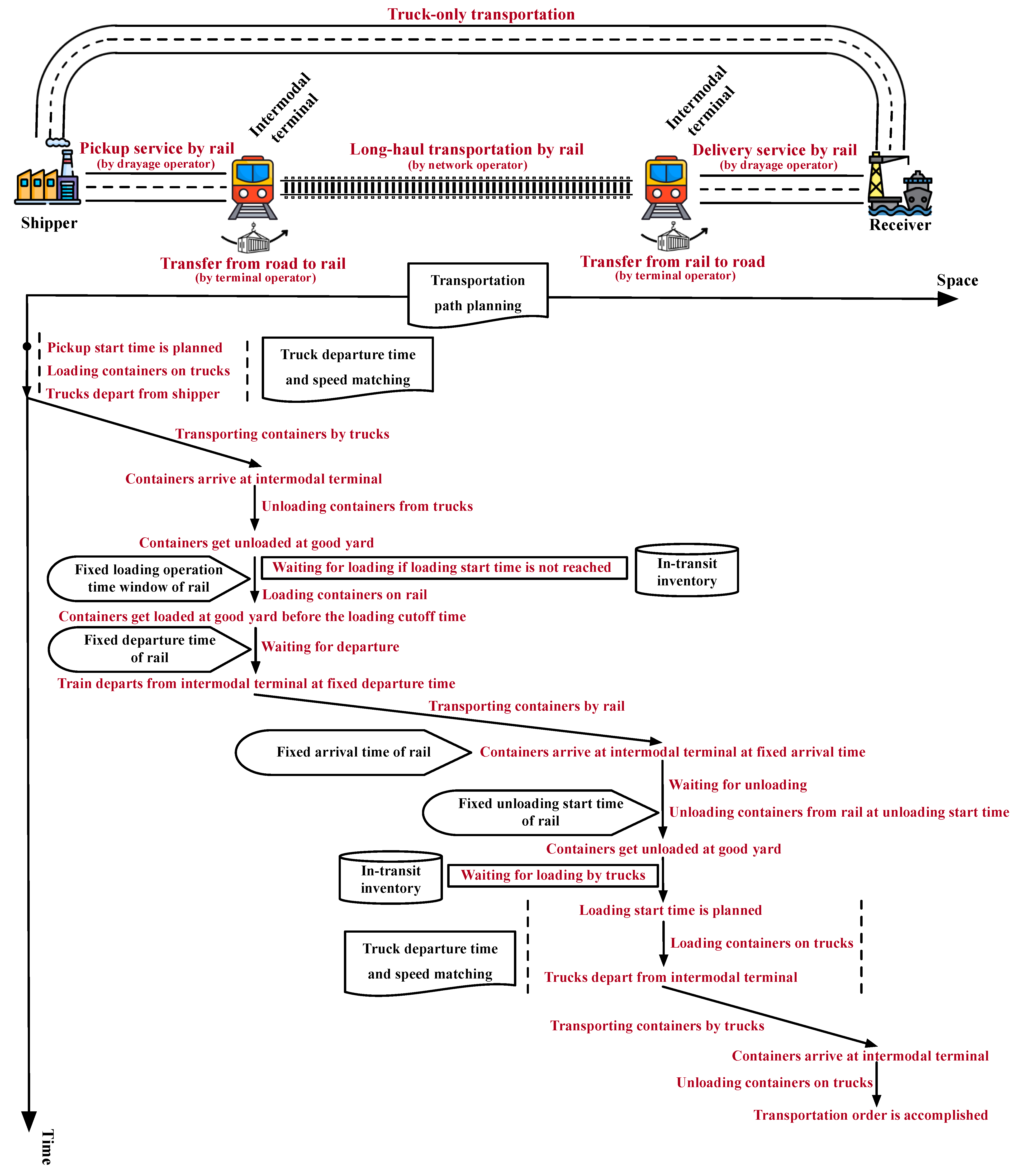
Figure 1. RRIT system.
Systems 11 00403 g001
Figure 2. Time-dependent and fuzzy truck speed.
Systems 11 00403 g002
Figure 3. Emission rate function of the road concerning speed.
Systems 11 00403 g003
Figure 4. The fuzziness of the transfer process from road to rail.
Systems 11 00403 g004
Figure 5. Relationship among different fuzzy measures [50].
Systems 11 00403 g005
Figure 6. The distributions of M e φ ~ β and M e φ ~ β concerning β .
Systems 11 00403 g006
Figure 7. Pareto solutions to the multi-objective RRIRP.
Systems 11 00403 g007
Figure 8. CO2 emissions with extensively raised carbon tax rates.
Systems 11 00403 g008
Figure 9. Travel costs of the Pareto solutions.
Systems 11 00403 g009
Figure 10. In-transit inventory costs of the Pareto solutions.
Systems 11 00403 g010
Figure 11. Time window violation degrees of the Pareto solutions.
Systems 11 00403 g011
Figure 12. Sensitivity of the total costs concerning λ and α .
Systems 11 00403 g012
Figure 13. Sensitivity of the transportation costs concerning λ and α .
Systems 11 00403 g013
Figure 14. Sensitivity of the CO2 emissions concerning λ and α .
Systems 11 00403 g014
Figure 15. Sensitivity of the time window violation degrees concerning λ and α .
Systems 11 00403 g015
Figure 16. Sensitivity of the travel costs concerning λ and α .
Systems 11 00403 g016
Figure 17. Sensitivity of the loading/unloading operation costs concerning λ and α .
Systems 11 00403 g017
Figure 18. Sensitivity of the in-transit inventory costs concerning λ and α .
Systems 11 00403 g018
Table 1. Notations.
Table 1. Notations.
Sets, Indices, and Parameters of the Transportation Orders
K Set of transportation orders served by the intermodal operator.
k Index   of   a   transportation   order ,   and   k K .
q k Demand   in   TEU   of   the   containers   of   transportation   order   k .
τ k ,   τ k + Origin - to - destination   pair   of   transportation   order   k   where   τ k   and   τ k + are the origin and destination nodes, respectively.
a k ,   a k + Soft   pickup   time   window   of   the   shipper   of   transportation   order   k .
b k ,   b k + Soft   delivery   time   window   of   the   receiver   of   transportation   order   k .
Sets and indices of the transportation network
N ,   A ,   S A   RRIT   network ,   where   N   is   the   node   set ,   A   is   the   directed   arc   set ,   and   S is the transportation service set.
h ,   i ,   a n d   j Indices   of   nodes ,   and   h ,   i , a n d   j N .
N i Set   of   the   predecessor   nodes   to   node   i ,   and   N i N .
N i + Set   of   the   successor   nodes   to   node   i ,   and   N i + N .
i ,   j A   directed   arc   from   node   i   to   node   j ,   and   i ,   j A .
r   a n d   s Indices   of   transportation   services ,   and   r   a n d   s S .
S i j = Π i j Γ i j Set   of   transportation   services   on   arc   i ,   j ,   and   Π i j   and   Γ i j are the sets of rail services and road services on the arc, respectively.
P i j s Set   of   continuous   time   ranges   for   road   service   s   on   arc   i ,   j .
p Index   of   a   time   range ,   and   p P i j s .
Parameters of the transportation services
d i j s Travel   distance   in   km   of   transportation   service   s   running   from   node   i   to   node   j .
t i s Loading / unloading   operation   time   in   hr / TEU   of   transportation   service   s   at   node   i .
[ l i s , l i s + ] Fixed   loading / unloading   operation   time   window   of   rail   service   s   at   node   i .
ϖ ~ i j s Trapezoidal   fuzzy   capacity   in   TEU   of   rail   service   s   on   arc   i ,   j ,   and   ϖ ~ i j s = ϖ i j s 1 ,   ϖ i j s 2 ,   ϖ i j s 3 ,   ϖ i j s 4 .
o i j s p ,   o i j s p + Interval   of   time   range   p   of   road   service   s   on   arc   i ,   j .
v ~ i j s p Trapezoidal   fuzzy   average   speed   in   km / hr   of   road   service   s   running   from   node   i   to   node   j   when   its   trucks   depart   from   node   i   in   time   range   p ,   and   v ~ i j s p = v i j s p 1 ,   v i j s p 2 ,   v i j s p 3 ,   v i j s p 4 .
e i j s CO 2   emission   rate   in   kg / TEU / km   of   rail   service   s   on   arc   i ,   j .
e ~ i j s p Speed - dependent   and   trapezoidal   fuzzy   CO 2   emission   rate   in   kg / TEU / km   of   road   service   s   on   arc   i ,   j   in   time   range   p ,   and   e ~ i j s p = e i j s p 1 ,   e i j s p 2 ,   e i j s p 3 ,   e i j s p 4 .
Parameters of costs
c r o a d 1 Travel cost rate in CNY (Chinese Yuan)/TEU/km of road services carrying out pickup and delivery services in the intermodal transportation.
c r o a d 2 Travel cost rate in CNY/TEU/km of truck-only transportation service.
c r a i l 1   a n d   c r a i l 2 Travel   cos t   rates   of   rail   services   where   c r a i l 1   is   the   rate   in   CNY / TEU   and   c r a i l 2   is   the   rate   in   CNY / TEU / km .   The   combination   of   c r a i l 1   and   c r a i l 2 determines the travel costs of rail services.
c s Loading / unloading   operation   cos t   rate   in   CNY / TEU   of   transportation   service   s .
c s t o r e Inventory cost rate in CNY/TEU/hr of intermodal terminals.
π An inventory period in hr that is free of charge at intermodal terminals.
c p e n a l t y Penalty cost rate in CNY/TEU/hr for violating the soft pickup or delivery time windows.
c e m i s s i o n Carbon tax rate in CNY/kg.
Auxiliary parameter and index
ξ A sufficient big number.
θ Index   of   a   prominent   point   of   a   trapezoidal   fuzzy   number ,   and   θ 1 ,   2 ,   3 ,   4 .
Deterministic variables
x i j s k 0 1   binary   variable   representing   the   use   of   a   specific   transportation   service   by   a   transportation   order .   x i j s k = 1   means   that   transportation   service   s   on   arc   i ,   j   is   used   to   move   the   containers   of   transportation   order   k ;   x i j s k = 0 otherwise.
u i j s p k 0 1   binary   variable   representing   the   use   of   a   specific   road   service   in   a   specific   time   range   by   a   transportation   order .   u i j s p k = 1   means   that   road   service     on   arc   i ,   j   in   time   range   p   is   used   to   move   the   containers   of   transportation   order   k ;   u i j s p k = 0 otherwise.
w k Non - negative   variable   representing   the   pickup   start   time   ( i . e . ,   the   time   when   the   containers   start   to   be   loaded )   of   transportation   order   k   at   its   origin   node   τ k .
g i k Non - negative   variable   representing   the   start   time   of   loading   containers   of   transportation   order   k   on   trucks   at   node   i .
n i j s k Non - negative   integer   variable   representing   the   day   that   road   service   s   departs   from   node   i   when   moving   the   containers   of   transportation   order   k   on   arc   i ,   j .
ϑ i j s k Non - negative   variable   representing   the   charged   in - transit   inventory   period   in   hr   of   the   containers   of   transportation   order   k   at   node   i   before   being   moved   being   moved   from   node   i   to   node   j   by   transportation   service   s .
δ k Non - negative   variable   representing   the   violation   in   hr   of   pickup   start   time   w k   of   transportation   order   k   regarding   a k ,   a k + .
Trapezoidal fuzzy variables
y ~ i k Non - negative   trapezoidal   fuzzy   variable   representing   the   time   when   the   containers   of   transportation   order   k   arrive   and   get   unloaded   at   node   i   using   road ,   and   y ~ i k = y i k 1 , y i k 2 ,   y i k 3 , y i k 4 .
z ~ i j s k Non - negative   trapezoidal   fuzzy   variable   representing   the   in - transit   inventory   period   in   hr   of   the   containers   of   transportation   order   k   at   node   i   before   being   moved   from   node   i   to   node   j   by   rail   service   s ,   and   z ~ i j s k = z i j s k 1 , z i j s k 2 ,   z i j s k 3 , z i j s k 4
m ~ i j s k Non - negative   trapezoidal   fuzzy   variable   representing   the   charged   in - transit   inventory   period   in   hr   of   the   containers   of   transportation   order   k   at   node   i   before   being   moved   from   node   i   to   node   j   by   rail   service   s ,   and   m ~ i j s k = m i j s k 1 , m i j s k 2 ,   m i j s k 3 , m i j s k 4
η ~ k Non - negative   trapezoidal   fuzzy   variable   representing   the   violation   in   hr   of   the   trapezoidal   fuzzy   delivery   accomplishment   time   of   transportation   order   k   regarding   b k ,   and   η ~ k = η k 1 ,   η k 2 ,   η k 3 ,   η k 4 .
μ ~ k Non - negative   trapezoidal   fuzzy   variable   representing   the   violation   in   hr   of   the   trapezoidal   fuzzy   delivery   accomplishment   time   of   transportation   order   k   regarding   b k + ,   and   μ ~ k = μ k 1 ,   μ k 2 ,   μ k 3 ,   μ k 4 .
Table 2. Transportation orders in the empirical case.
Transportation Order No.Demands (TEU)Soft Pickup Time WindowsSoft Delivery Time Windows
122[10, 15][95, 105]
220[20, 28][140, 150]
315[13, 20][130, 139]
417[18, 25][85, 94]
534[28, 35][88, 98]
615[12, 17][110, 120]
723[30, 35][135, 141]
830[36, 41][142, 152]
933[14, 20][104, 112]
1025[22, 30][131, 140]
Table 3. Values of the cost- and time-related parameters in the empirical case.
Cost ParametersValuesData Sources
c r o a d 1 6.0 CNY/km/TEUMinistry of Transport of China and National Development and Reform Commission of China
c r o a d 2 9.256 CNY/km/TEU
c s 25 CNY/TEU for road
195 CNY/TEU for railChina State Railway Group Company
c r a i l 1 440 CNY/TEU
c r a i l 2 3.185 CNY/km/TEU
c s t o r e 3.125 CNY/km/hr
c p e n a l t y 5 CNY/TEU/hrSet by this study
Time parametersValuesData sources
t i s 0.2 CNY/TEU for railResat and Turkay [25]
0.05 CNY/TEU for road
π 6 hrSet by this study
Table 4. Computational scale of the empirical case.
VariablesInteger VariablesConstraints
379912518343
Table 5. Optimization results under different carbon tax rates.
Tax Rates (CNY/t)Total Costs (CNY)Emissions
(kg)
F 1
(CNY)
F 2
(CNY)
E F ~ 3
(CNY)
Time Window violation Degrees
(TEU·hr)
CPU Time
(s)
102,499,379569,5462,412,65537,2204800780267
202,505,075569,5462,412,65537,22048007802101
302,510,770569,5462,412,65537,22048007802111
402,516,994565,6922,412,65537,2205327783369
502,522,161569,5462,412,65537,22048007802298
602,527,741547,0122,412,65537,22051017989137
702,533,712561,2492,412,65537,2205328784583
802,538,630534,9042,412,65537,2205627806773
902,544,777545,3882,412,65537,2205627803840
1002,549,347521,2882,412,65537,2205818830515
Disclaimer/Publisher’s Note: The statements, opinions and data contained in all publications are solely those of the individual author(s) and contributor(s) and not of MDPI and/or the editor(s). MDPI and/or the editor(s) disclaim responsibility for any injury to people or property resulting from any ideas, methods, instructions or products referred to in the content.