

Energy-Saving Scheduling for Flexible Job Shop Problem with AGV Transportation Considering Emergencies
by
 , , and
Hongliang Zhang
1,
Chaoqun Qin
1,
Wenhui Zhang
2,
Zhenxing Xu
1,
Gongjie Xu
3,4,* and
Zhenhua Gao
1 1
School of Management Science and Engineering, Anhui University of Technology, Ma’anshan 243002, China
2
Department of Mechanical and Electrical Engineering, Hebei Construction Marterial Vocational and Technical College, Qinhuangdao 066004, China
3
Performance Analysis Center of Production and Operations Systems (PacPos), Northwestern Polytechnical University, Xi’an 710072, China
4
Department of Industrial Engineering, School of Mechanical Engineering, Northwestern Polytechnical University, Xi’an 710072, China
*
Author to whom correspondence should be addressed.
Systems 2023, 11(2), 103; https://doi.org/10.3390/systems11020103
Submission received: 10 January 2023
/
Revised: 31 January 2023
/
Accepted: 7 February 2023
/
Published: 13 February 2023
(This article belongs to the Topic Advances in Renewable Energy Technologies and Systems Solutions)
Abstract
:Emergencies such as machine breakdowns and rush orders greatly affect the production activities of manufacturing enterprises. How to deal with the rescheduling problem after emergencies have high practical value. Meanwhile, under the background of intelligent manufacturing, automatic guided vehicles are gradually emerging in enterprises. To deal with the disturbances in flexible job shop scheduling problem with automatic guided vehicle transportation, a mixed-integer linear programming model is established. According to the traits of this model, an improved NSGA-II is designed, aiming at minimizing makespan, energy consumption and machine workload deviation. To improve solution qualities, the local search operator based on a critical path is designed. In addition, an improved crowding distance calculation method is used to reduce the computation complexity of the algorithm. Finally, the validity of the improvement strategies is tested, and the robustness and superiority of the proposed algorithm are verified by comparing it with NSGA, NSGA-II and SPEA2.
1. Introduction
Flexible job shop scheduling problem (FJSP) has been a hot topic in recent years. Compared with traditional job shops, flexible job shops embody production flexibility [1]. For the actual production environment to be dynamic, it is essential to consider the impact of dynamic events when making production scheduling plans. Machine breakdowns and rush orders are common disturbances in manufacturing enterprises. Inappropriate environmental factors, such as dust, temperature, corrosion, climate, as well as improper operation of the machine, may lead to breakdowns. Moreover, rush orders also often occur in enterprises, and the reasons for inserting rush orders mainly include inharmonious coordination among departments and deviations in sales forecast. To obtain the maximum benefits or minimize losses, decision-makers need to make adjustments to the existing production plan in response to the disturbances. In order to alleviate the impact of disturbances on scheduling decisions, the FJSP considering machine breakdowns and rush orders has attracted the attention of scholars.
FJSP has been proven to be an NP hard problem [2]; the FJSP with machine breakdown is more complex. Due to the complexity of the problem, the traditional operational research methods find it difficult to obtain good results, so swarm intelligence optimization algorithms are adopted by scholars in solving this problem. From the perspective of optimization objectives, related studies can be divided into single-objective and multiple-objective optimization problems. For single-objective optimization problems, makespan is the main optimization objective of this problem. Aiming to minimize makespan, Tang et al. [3] considered machine breakdowns and proposed a rescheduling prediction method. Li et al. [4] proposed an adaptive hybrid genetic-brain storm optimization algorithm for FJSP with machine breakdown. With the goal of minimizing the number of delayed jobs, Mokhtari et al. [5] proposed an optimization framework based on simulated annealing and Monte Carlo simulation for FJSP with machine breakdowns. As for multi-objective optimization to this problem, in addition to makespan, the stability and robustness of the model are considered by scholars. Ahmadi et al. [6] proposed an NSGA-II and an NRGA aiming at minimum makespan and maximum stability simultaneously. With the goals of minimizing makespan and maximizing robustness, Yang et al. [7] designed an NSGA-II integrating extreme learning machine for FJSP with machine breakdown. You et al. [8] proposed an NSGA-II with game theory for this problem. Zhang et al. [9] proposed an improved convolutional neural network, aiming at minimizing makespan and robustness for the problem. Jin et al. [10] proposed a rescheduling method integrating simulation, genetic optimization and neural network with the goals of minimizing makespan difference, operation completion time difference and variable cost.
As for FJSP considering rush orders, scholars have proposed metaheuristic optimization algorithms. Gao et al. [11] proposed an improved artificial bee colony algorithm for the FJSP with rush orders considering fuzzy processing time. Zhang et al. [12] proposed a combination of variable neighborhood search and gene expression programming algorithms with four effective neighborhood structures.
The above studies have designed effective methods for the FJSP with machine breakdown or rush order arrival. Considering only single disturbance factors has certain limitations in practice. However, in actual production, both of them may occur at the same time, so it is necessary to integrate these two factors.
Recently, the FJSP integrating machine breakdowns and rush orders have received the attention of scholars. In order to solve the multi-objective dynamic FJSP, Shen et al. [13] proposed a proactive–reactive method based on a multi-objective evolutionary algorithm and designed a dynamic decision-making program to choose the best scheduling scheme. Wang et al. [14] proposed a multi-objective differential evolution algorithm for the dynamic FJSP considering machine breakdowns and rush orders. Baykasoğlu et al. [15] studied the dynamic FJSP under uncertain events, including new order arrivals and machine breakdowns, and designed a constructive algorithm adopting a greedy randomized adaptive search procedure. The above studies studied the FJSP from event disturbance scenarios, but ignored the factors of energy conservation and emission reduction. In order to comply with green and sustainable development, energy consumption should be taken into account.
As for energy-saving FJSP considering a single disturbance, Zhang et al. [16] proposed an improved empire competition algorithm for FJSP with machine breakdowns, aiming at minimizing makespan, energy consumption and total delay time. Considering the impact of machine breakdowns in FJSP, Duan et al. [17] designed an improved NSGA-II based on real number coding with the goals of minimizing makespan and energy consumption. Caldeira et al. [18] designed an improved backtracking search algorithm for FJSP with rush orders, considering minimal makespan, minimal energy consumption and maximal robustness. Moreover, energy-saving FJSP with multiple disturbances also received attention. Li et al. [19] established a model for FJSP considering machine breakdowns and rush orders with the goals of minimizing makespan, total energy consumption and maximizing robustness. Duan et al. [20] proposed a multi-objective PSO algorithm, aiming to minimize total energy consumption, makespan and maximize the comprehensive reusability of the system.
To sum up, the majority of studies on FJSP with disturbances are limited to a single disturbance factor, and the studies considering AGV transportation in FJSP with multiple disturbances are scarce. With the development of intelligent manufacturing, AGVs have been adopted in many industries to implement material transportation, such as home appliance production, microelectronics manufacturing, cigarette, chemical industry and other industries, so the role of AGVs cannot be ignored. Under the background of energy saving and dynamic event disturbance, this article addresses energy-saving scheduling for FJSP with AGV transportation considering the machine breakdown and rush order (FJSP-AMBRO). The major contributions of this article are as follows: (1) considering the disturbances, a mixed-integer linear programming model is established for the FJSP-AMBRO problem; (2) to minimize the makespan, total energy consumption and workload deviation of equipment, an improved NSGA-II (INSGA-II) is designed; (3) due to the complexity of the original crowding distance calculation, a new crowding distance calculation method is proposed to reduce the computational complexity of the algorithm; (4) in order to increase the local search ability and obtain better solutions, a local search strategy based on critical path transformation is adopted in the algorithm.
The rest of the article is organized as follows. In Section 2, the FJSP-AMBRO is formulated in detail and a mixed-integer linear programming model is presented. The improved NSGA-II is illustrated in Section 3. The orthogonal experiment, validity verification of the improvement strategies, comparison experiments and result analysis are described in Section 4. In Section 5, conclusions and future research directions are given.
2. Problem Description
2.1. Introduction of FJSP-AMBRO
In FJSP-AMBRO, there are n jobs J = {, ,…, } and m machines M = {, ,…, }, the job has operations, the process route of each job may be different, and there may be multiple machines available for each operation. Different machines may have different power. g AGVs A = {, ,…, } are used in the workshop to transport the jobs. During the production process, rush orders and machine breakdowns may occur randomly. For instance, an example of parameters (n = 2, m = 2, g = 3, = 3, = 4) represents that there are two machines in the workshop, two jobs need to be processed and the number of operations for two jobs is three and four, respectively, four AGVs are responsible for the transportation of jobs in the workshop. The purpose is to reasonably plan the processing sequence of the jobs, the processing machine and the AGV transportation distribution so that the scheme can achieve the expected goal.
In order to facilitate the establishment of the model, the following assumptions are proposed:
- (1)
- Each machine can only process one job at the same time.
- (2)
- Each job can only be processed on one machine at a time.
- (3)
- All AGVs, jobs and machines are ready at time 0.
- (4)
- The AGV can proceed to the next task only after completing the current task.
- (5)
- An AGV can only carry one job at one time.
- (6)
- Ignore the power of AGVs; all AGVs have the same speed.
- (7)
- The collision of AGVs are ignored.
- (8)
- The maintenance time of the broken machine is known.
- (9)
- The arrival time of rush orders, the job number in rush orders are random and the rush orders have processing priority. The machine breakdown and the rush order occur only once, respectively.
- (10)
- AGVs and raw materials are in the warehouse at time 0, and AGVs will drive to the finished product warehouse after completing the transportation tasks.
There are three situations when a breakdown occurs: (1) there is a job being processed on the faulty machine, which needs to be suspended and then reprocessed until the faulty machine is maintained. The unprocessed operations after the machine breakdown will be rearranged; (2) all machines are in the no-load state, but the jobs are not completed, all unprocessed operations after the breakdown will be rearranged; (3) all jobs are finished, and there is no need to reschedule the scheme.
Similarly, when a rush order arrives, one of the following situations will occur: (1) there is at least one operation being processed at the arrival time of a rush order. The operation being processed will be suspended and then reprocessed after finishing the rush order. The rush order occupies processing priority, and original unprocessed operations will be rescheduled after finishing the rush order; (2) all machines are in the no-load state, and the original order is not completed. The rush order will be carried out directly. After completion of the rush order, the remaining operations of the original order will be rescheduled and processed; (3) the original order has been completed, only the rush order needs to be rescheduled and processed.
Compared with other studies on FJSP considering disturbances, AGV transportation is introduced, and various transportation situations in the workshop of AGVs are considered in this article. During the production with no disturbance, there are two situations: I. if an AGV is assigned a transportation task, and the job that will be transported is being processed when the AGV reaches the job position, the AGV needs to wait until the operation is finished, as shown in Figure 1a. II. an AGV executes two consecutive transportation tasks for the same job. After completing the first transportation task, the job will be unloaded on the corresponding machine for processing, and the AGV will wait for the completion of the operation and then continue to execute the next transportation of this job, as shown in Figure 1b.
When the disturbance events occur, the subsequent production plan is adjusted, and the transportation tasks of AGVs also need to be rearranged. If a machine breaks down, the transportation tasks after the breakdown will be canceled, as shown in Figure 1c. After the AGV arrives at the faulty machine, three situations may occur: I. if the job, which is unloaded from the AGV or has been interrupted on the faulty machine, is replaced with another machine for processing after rearrangement, the AGV will immediately transport the job to the replaced machine, as shown in Figure 1d,e; II. if the job is still processed on the faulty machine after rearrangement, it will be processed after remedying the breakdown; the AGV will leave to execute the next task after unloading the job, as shown in Figure 1f; III. if the job will still be processed on the faulty machine after rearrangement and the next transportation task of the job will be performed by the same AGV, the AGV needs to wait here for the machine breakdown to be cleared and finish the next operation, then transport the job to the next position, as shown in Figure 1g,h.
When the rush order arrives, the subsequent tasks of AGVs will be deleted, as shown in Figure 1i. The AGV will arrive at the next position and abandon the current transportation task, then immediately return to the raw material warehouse to transport the rush order jobs for processing, as shown in Figure 1j.
On the basis of the FJSP problem, the factors of AGV transportation, the machine breakdown and the rush order are considered. In addition to makespan, energy consumption and machine load deviation are set as optimization objectives for the problem. As shown in Figure 2, there are obvious coupling relationships between constraints and goals of the problem, which greatly increase the difficulty of problem solving.
According to the preceding situations, the influence of disturbances is further considered, which makes the coupling relationship of various factors more complex. The occurrence of the machine breakdown directly interrupts the production and changes the AGV transportation start time, machine allocation and the start processing time of each operation, leading to the subsequent production plan no longer adapting to the target requirements, so the task sequence of operations, machines and AGVs must be rearranged. When the rush order arrives, the unfinished operations will be postponed. The arrival of the rush order increases the number of jobs, which, in turn, increases the number of tasks of machines and AGVs. Machines and AGVs need to readjust their tasks. Moreover, the two disturbances will also affect each other. The machine breakdown will limit the processing of jobs and AGV transportation of the rush order. The arrival of the rush order will also disrupt the rescheduling scheme after the machine breakdown. These factors interact with each other, making the FJSP-AMBRO become a high-dimensional and multi-objective optimization problem.
2.2. Symbol Definitions
To facilitate the establishment of the mathematical model, symbols are defined as shown in Table 1:
2.3. Mathematical Model
The mathematical model for FJSP-AMBRO is established as follows:
s.t.
Equations (1)–(3) are objective functions, which represent minimizing the makespan, energy consumption and sum of workload deviation, respectively. Constraint (4) indicates an operation can only be processed after the previous operation of the same job is completed. Constraint (5) indicates an operation can only be processed by one machine. Constraint (6) represents that a machine can only process one job at one time. Constraint (7) indicates a job can only be processed after being transported by the AGV to the corresponding machine. Constraint (8) indicates a job can only be transported after processing. Constraint (9) indicates a job can only be transported by one AGV at the same moment. Constraint (10) means that an AGV can only transport one job at one time. Equation (11) represents the energy consumption of the entire process.
3. Algorithm Design
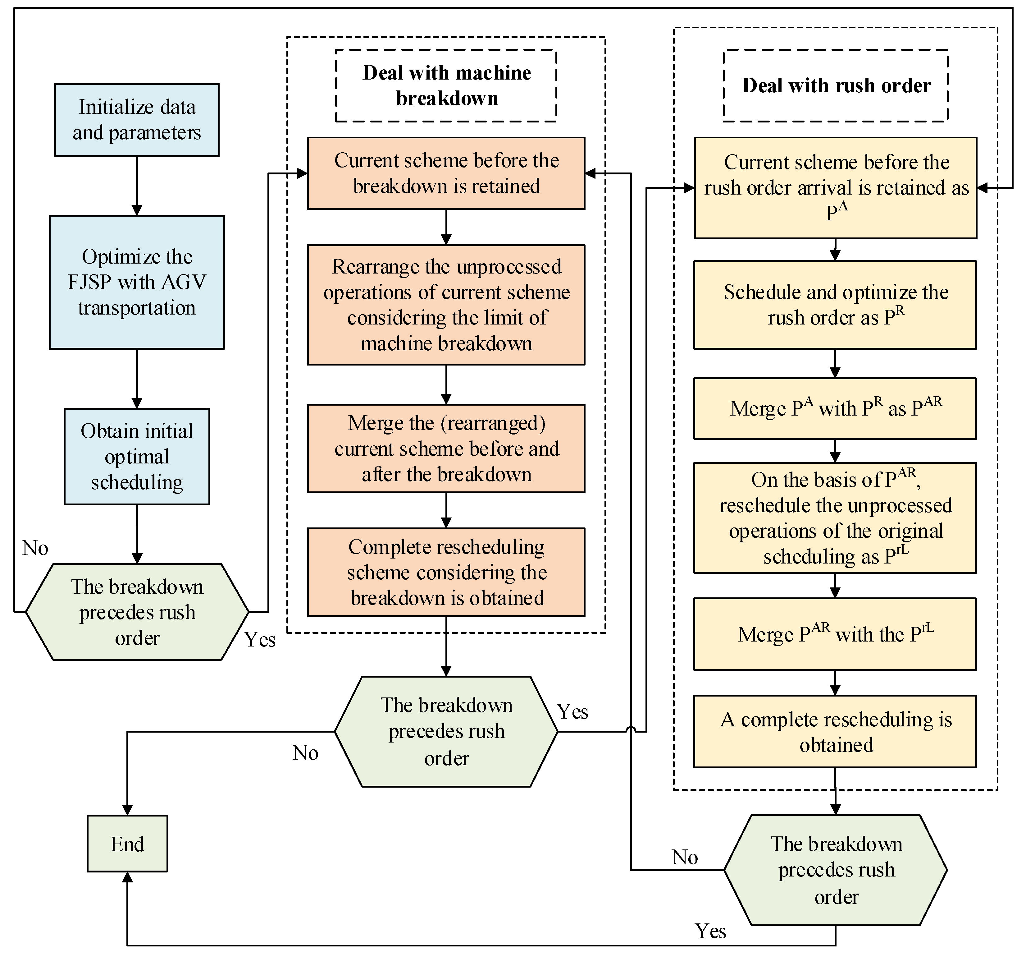
3.1. Emergency Handling Process for FJSP-AMBRO
For FJSP-AMBRO, the emergency handling process is shown by Figure 3. First, the problem model, without considering any disturbance, is optimized to obtain an initial optimal scheme for FJSP with AGV transportation. According to the occurrence sequence of machine breakdowns and rush orders, there are two cases. In case I, the breakdown occurs before or at the same time as the rush order; the processing steps are as follows: (1) the impact of the machine breakdown should be dealt with first. The initial scheme before the breakdown is retained, then the initial optimal scheme, which is at and after the moment of breakdown, is rearranged, and an optimal scheme considering the breakdown is received; (2) deal with the rush order, the current scheme is divided into two parts, before insertion and after insertion. Set the rush order with priority and the optimized rush order scheme as . Integrate and into a scheme . Then, is rearranged as , finally, is combined with to obtain the final scheduling scheme. In case II, the priority to deal with the rush order is higher than that of the machine breakdown.
3.2. Improved NSGA-II
For the advantages of strong robustness and global search ability, NSGA-II is widely applied in different practical multi-objective optimization problems by many researchers [21]. However, it still has the shortcomings of insufficient local search ability, and slow evolution speed [22]. In view of the shortcomings of NSGA-II and the high complexity of FJSP-AMBRO, the INSGA-II with the new crowding distance calculation method and local search strategy is proposed.
3.2.1. Three-Layer Encoding and Decoding
The encoding and decoding methods have a significant impact on the efficiency of the algorithm. For FJSP-AMBRO, a three-layer encoding method is adopted, including operation sequence (OS), machine sequence (MS) and AGV sequence (AS), illustrated in Figure 4. Each gene of OS indicates the job index, and the occurrence number of the job index indicates the index of its operation. The MS indicates the processing machine of the corresponding operation. AS represents the AGV index required to transport the corresponding job. The decoding process converts the encoding into a scheduling scheme.
3.2.2. Selection Operator with Improved Crowding Distance Calculation
To better preserve the excellent solution in the population, the elite retention strategy [23] is adopted in the selection operation. The non-dominated sorting is complex. The selection operation is time-consuming in the algorithm. The traditional crowding distance calculation method has high computation complexity, which may reduce the speed of the algorithm. An improved crowding distance calculation method is proposed in this article, which can reduce the computational complexity and accelerate evolution. The formula of the proposed crowding distance is expressed as Equation (12):
where is the i-dimensional target value of the point, is the center coordinate of all points in the solution space, and m is the dimension of the target. Equation (13) represents the i-dimensional calculation method for the center of gravity.
where N represents the number of solutions and is the i-dimensional target value of the a-th solution.
After improvement, each individual in the population only needs to perform one operation on each target in the selection operator, which greatly simplifies the operation. Specifically, the computational complexity of the traditional crowding degree is O() [24], where m is the number of objects and N is the population size. In this article, a distribution center of a solution set is calculated, and each solution is compared with the distribution center to determine its quality. Compared with the pair-wise comparison of traditional non-dominated sorting, the proposed method reduces the computational complexity to O(mN) in this article.
3.2.3. POX Crossover Operation
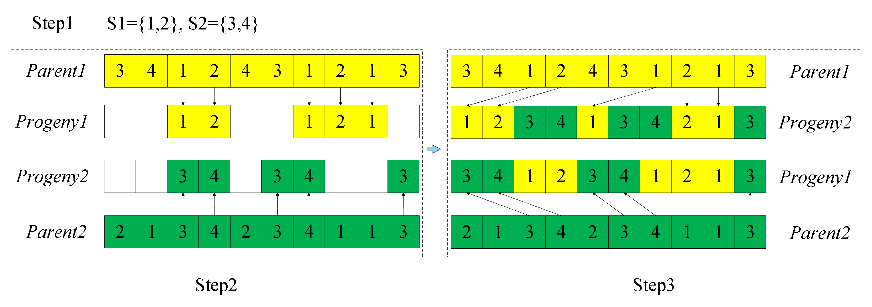
Crossover is one of the most important ways to generate new individuals, which can preserve part of the individual genes and enhance population diversity. According to the characteristics of this problem, POX crossover is adopted in this article. POX crossover [25] is a commonly used crossover method for its high efficiency. The basic steps of POX crossover for OS are shown in Algorithm 1, and the schematic diagram is shown in Figure 5.
| Algorithm 1: Procedure of POX crossover operation |
| 1: Select two parent individuals. 2: classify the jobs into sets S1 and S2. 3: The genes in set S1 of Parent1 are inherited to the same position of Progeny1. 4: The genes in set S2 of Parent2 are inherited to the same position of Progeny2. 5: The rest positions of genes in progenies are temporarily vacant. 6: The remaining genes in Parent1 are filled into the empty positions of Progeny2 in order. 7: The remaining genes in Parent2 are filled into the empty positions of Progeny1 in order. |
3.2.4. Three-Layer Mutation Operator
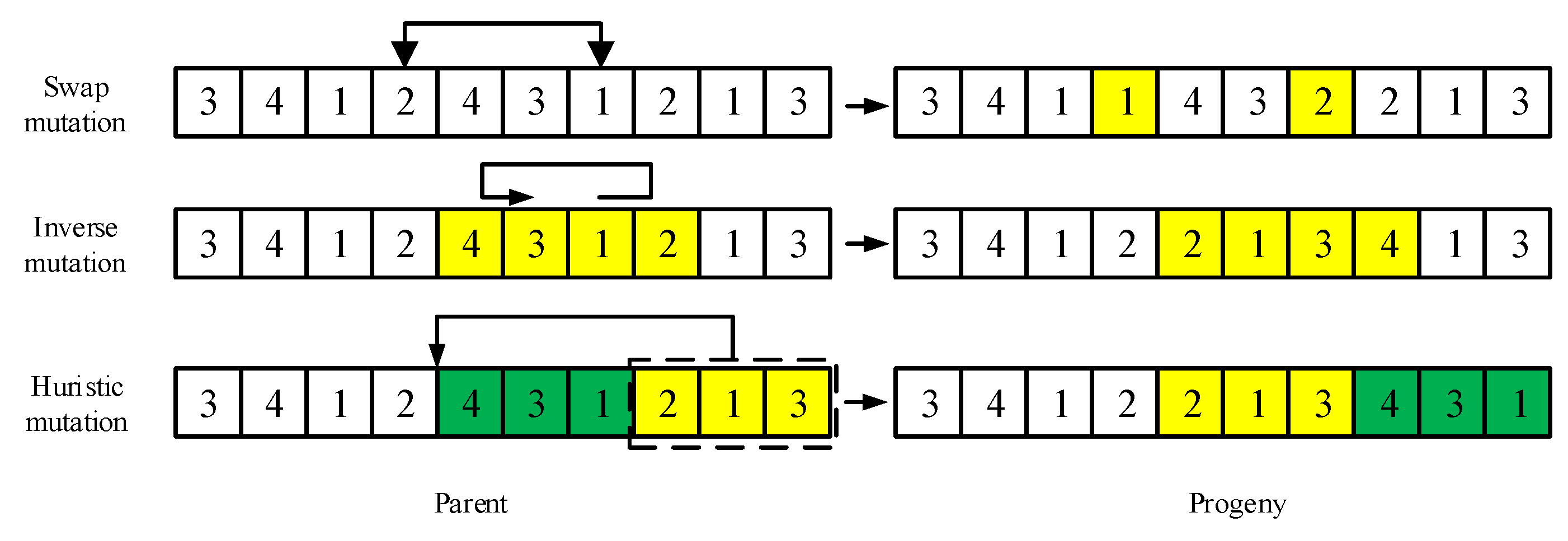
Mutation is an important operation for algorithms to avoid entering local optimization and ensuring evolution from multiple directions, thus promoting global search capabilities. In the three-layer encoding, OS and MS have obvious interaction. Unsuitable MS will lead to an unfeasible solution. As AGVs can transport any job, AS is relatively independent of OS and MS. According to the encoding characteristics, the mutation methods are designed for OS, MS and AS, respectively. The procedure of three-layer mutation operator is shown as Algorithm 2. OS mutation includes swap mutation, inverse mutation and heuristic mutation [26]. Figure 6 shows the three mutation modes of OS.
| Algorithm 2: Procedure of three layer mutation operator |
| 1: Determine the number of mutation individuals mutate_num. 2: for i in range(mutate_num): 3: Generate a random decimal mutate_num_1 ∈ [0,1]. 4: Randomly select an individual Xi. 5: if rand_num_1 <1/3: 6: (Perform OS mutation.) 7: Generate a random decimal mutate_num_2 ∈ [0,1]. 8: if rand_num_2 <1/3: 9: Perform swap mutation on Xi. 10: elif rand_num_2 <2/3: 11: Perform inverse mutation on Xi. 12: else: 13: Perform heuristic mutation on Xi. 14: Regenerated MS to ensure the feasibility of solutions 15: elif rand_num_1 <2/3: 16: (Perform MS mutation.) 17: Generate a random decimal mutate_num_3 ∈ [0,1]. 18: if rand_num_3 <1/2: 19: (Perform directional mutation on Xi.) 20: Randomly select a position in MS of Xi. 21: Reselect an available machine with the shortest processing time. 22: else: 23: (Perform random mutation on Xi.) 24: Randomly select a position in MS of Xi and randomly reselect an available machine. 25: else: 26: (Perform AS mutation.) 27: Randomly select a different AGV to replace the original one of Xi. |
3.2.5. Local Search Based on Critical Path
In order to enhance the local search ability of the algorithm and obtain better solutions, the critical path operation block transformation strategy [27] is adopted in the literature. Combined with the characteristics of this problem, a local search strategy based on the critical path operation block transformation considering AGV transportation is proposed.
On the critical path, if three or more consecutive operations are on the same machine, these consecutive operations are called a critical path operation block. Adjusting the operation sequence in an operation block may shorten the makespan. When in the operation block moves forward, an idle time interval is needed on the processing machine of before the corresponding AGV transportation start time of . For example, as shown in Figure 7, the critical path is the operation path composed of ------. is inserted in front of in the critical path operation block, then with AGV transportation process has an advance-vacancy of time interval t on M1. After transformation, the critical path changed to ---–-- and the idle time between and is reduced. Therefore, makespan is reduced by time interval t, and the transformation is effective.
4. Experimental Analysis
All algorithms in this article are programmed on PyCharm Community Edition 2019.2 software and run on Windows 7 operating system configured with an Intel(R) Core (TM) i7-4790CPU and 3.60 GHz/4GB RAM.
4.1. Example and Performance Metrics
Due to the lack of standard examples for FJSP-AMBRO, the expanded examples are obtained on the basis of Brandimarte’s data set [28]. For each example oinBrandimarte’s data set, the machine breakdown and the rush order occur once. A total of 20–40% jobs of each example are randomly selected in the rush order. The breakdown duration is 20 to 100 s on a random machine.
In this article, inverted generational distance (IGD) [29] and set coverage (C) [30] are used as performance metrics. IGD and C-metric reflect the distribution and convergence of solution sets, respectively. IGD is expressed as Equation (14):
where PF is the Pareto front obtained by the algorithm, and PF* is the real Pareto front. represents the size of PF*. d(,) is the distance between and in solution space. A smaller IGD value means a better PF is obtained by the algorithm.
C-measure can be expressed as Equation (15):
where and are the Pareto fronts obtained by method 1 and method 2, respectively, and is the size of . A larger C-metric value means better Pareto front .
4.2. Parametric Analysis
Parameters are the key factors affecting algorithm performance. The Taguchi experiment is a multi-factor and multi-level experimental design method. When the test involves multiple factors and there may be interactions between them, the Taguchi experiment can achieve results equivalent to a large number of comprehensive tests with a minimum number of tests. Therefore, the Taguchi experiment can quickly determine the reasonable parameter values of the algorithm. The proposed INSGA-II can be divided into two parts: the initial scheduling optimization and rescheduling optimization, so it is necessary to determine the parameters for the two parts. MaxIt1, PC1 and PM1 are the max iteration, crossover probability and mutation probability of initial optimization, respectively, and MaxIt2, PC2 and PM2 are the parameters of the rescheduling optimization. is used as the orthogonal table of experiment and a total of 25 groups of experiments are required. The parameter level settings are shown in Table 2.
The extended example of Mk-08 is used as experimental data in the Taguchi experiment, and IGD is used as the experimental evaluation index. Each experiment is repeated 10 times, and the average value of the 10 results is taken as the performance metric. The results of the Taguchi experiment are shown in Table 3.
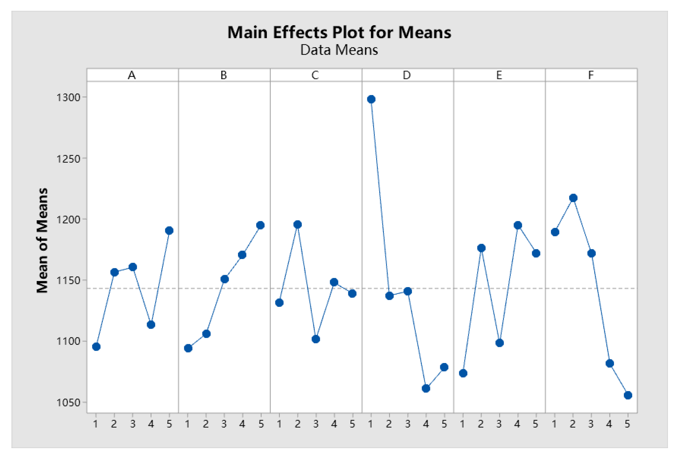
Based on the data in Table 3, the mean value of IGD-main effect response diagram is obtained as shown in Figure 8. From Figure 8, the optimal parameter values are fixed, and it is known that the proposed algorithm performs best when MaxIt1, PC1, PM1, MaxIt2, PC2 and PM2 are 200, 0.40, 0.10, 500, 0.40 and 0.20, respectively.
4.3. Validity Analysis of Improvement Strategies and the Comparison Experiment
To reduce the impact of accidental errors, each algorithm is tested 20 times for each example in Brandimarte’s data set to verify the validities of the strategies and algorithm comparisons.
The validity of improved crowding calculation has been verified in Section 3.2.2. In order to verify the impact of the local search strategy on the solution quality of the algorithm, the experiments are executed by NSGA-II, NSGA-II with local search strategy () and INSGA-II, respectively. The results are shown in Table 4, where the bold values indicate that the results of are better than NSGA-II, and the bold values with down arrows mean the results of INSGA-II are further better than .
It can be seen from Table 4 that, for all 15 examples, the result shows that the IGD value of is smaller than that of NSGA-II. This shows that the local search strategy significantly improves the quality of the solutions. The IGD comparison from and INSGA-II shows the advantage of INSGA-II on performance, which further proves the validity of the local search strategy. The C-metric results reflect that the solution quality of is much better than NSGA-II, and INSGA-II also has certain advantages over in all 15 examples, which illustrates the effectiveness of the proposed strategy. To validate the significance of the difference, a pair-wise t-test with a 95% confidence interval for NSGA-II- and -INSGA-II is implemented, and the “sig.(2-tail)” values are both 0.003, less than 0.05, which confirms there are significant differences between NSGA-II and and and INSGA-II.
In this article, NSGA, NSGA-II and SPEA2 are selected as comparison algorithms. Table 5 lists the IGD values of INSGA-II and the other three comparison algorithms for each example. The real Pareto front PF* is found by synthesizing the Pareto front solutions obtained from all algorithms. It can be seen from Table 5 that compared with NSGA, NSGA-II and SPEA-II, the proposed INSGA-II can acquire better performances for all examples except Mk-02 and Mk-08.
Table 6 lists the C-metric value between INSGA-II and the other three comparison algorithms. It can be seen from Table 6 that the C-metric value of INSGA-II is greater than that of other algorithms in all examples, which shows that the optimization performance of INSGA-II is better.
In order to test whether the difference between the experimental results in Table 5 and Table 6 is statistically significant, this article conducts a t-test with a 95% confidence interval for the results obtained by INSGA-II and the other three algorithms. The results of the t-test are shown in Table 7, and it can be seen from this table that when the “Sig.(2-tailed)” value is less than 0.05, the result for each pair of algorithms in the corresponding row is significantly different. This reveals that INSGA-II is significantly superior to NSGA, NSGA-II and SPEA2.
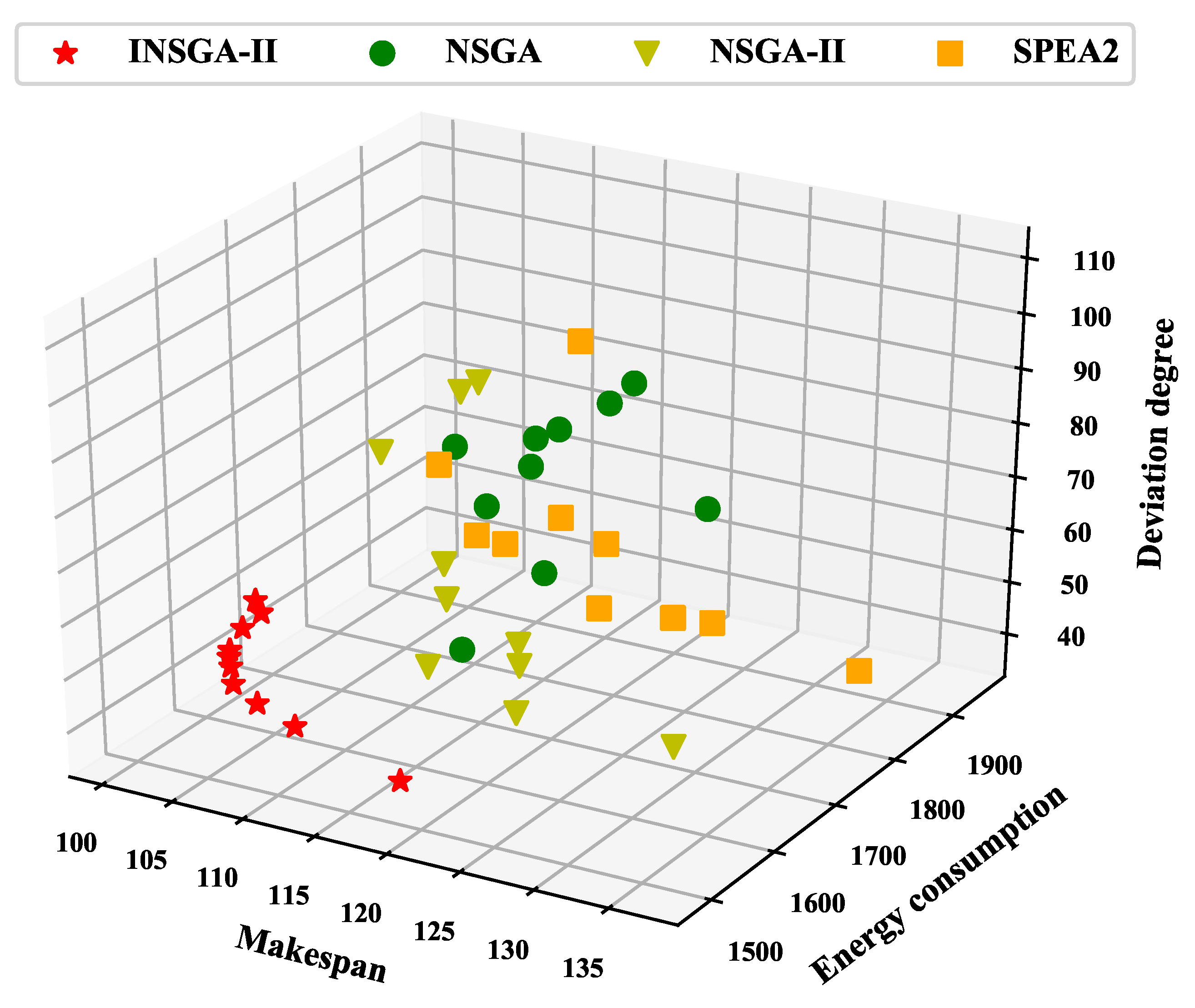
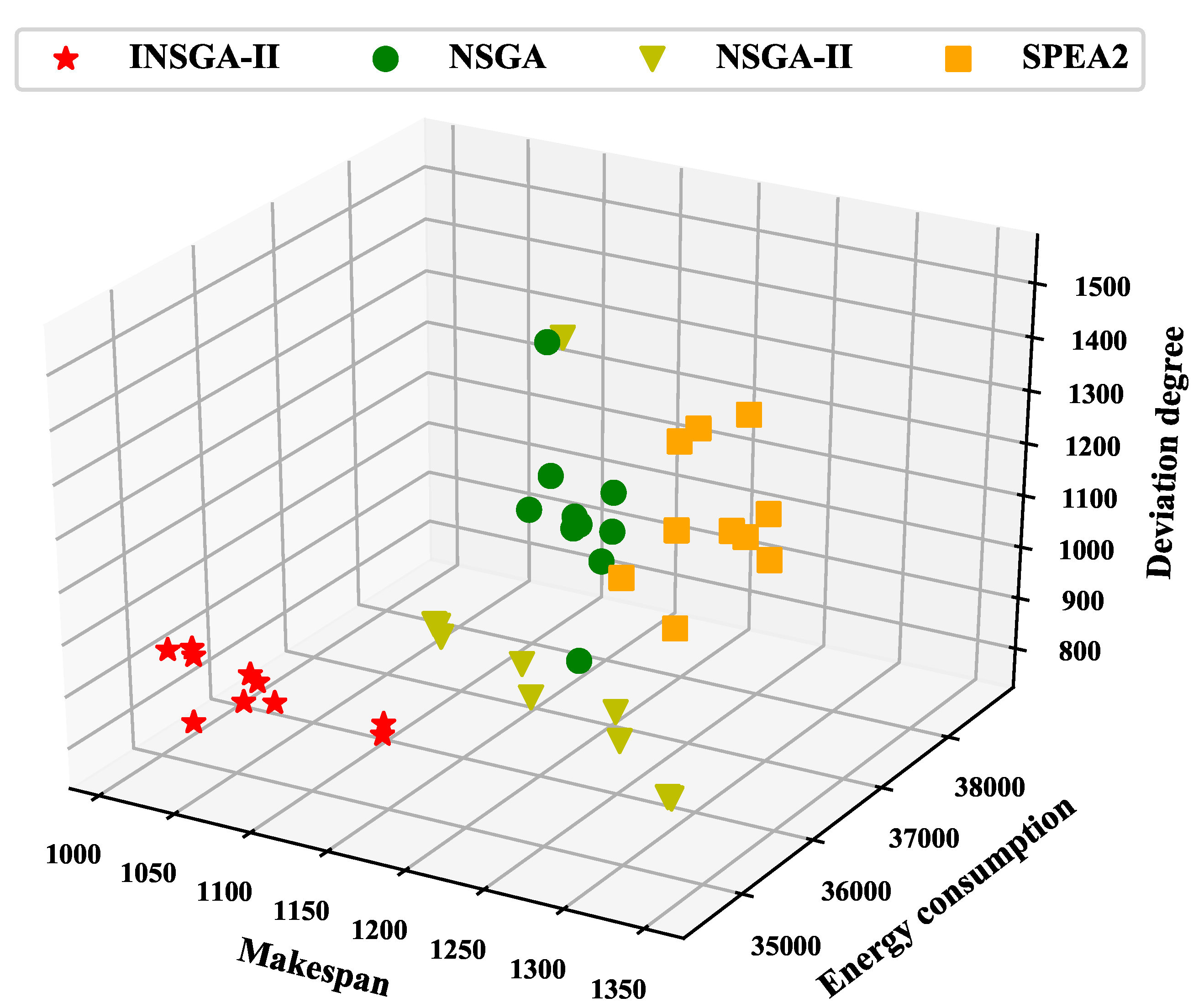
To observe the Pareto front distribution of each algorithm more intuitively, the distribution diagrams of solution sets obtained by four algorithms on Mk-01, Mk-05, Mk-10 and Mk-15, which represent examples with different scales, are drawn. As shown in Figure 9, Figure 10, Figure 11 and Figure 12, the solution set obtained by INSGA-II is significantly better than the other three comparison algorithms. The solutions of INSGA-II are closer to the origin in three dimensions of makespan, energy consumption and deviation, illustrating the superiority of INSGA-II.
From the above analysis, it can be seen that INSGA-II shows significant advantages in performance on most examples of Brandimarte’s data set. From the perspectives of IGD and C-metric, it is known that INSGA-II has a better performance than other algorithms.
From the above analysis, it is clear that the improved strategies enhance the performance of the proposed algorithm. The reasons leading to this result mainly include the following aspects. First, the selection operation integrating an elite retention strategy retains the high-quality solutions generated in the process of evolution. Secondly, the mutation with two directions avoids premature evolution. Thirdly, the local search strategy further searches for better solutions around the solution space of the high-quality solutions. Based on the local search of the operation block transformation, the idle time on machines in the workshop is reduced as much as possible by changing the operation sequence on the critical path so as to reduce the idle ratio and shorten the production cycle.
5. Conclusions
This article addresses the FJSP considering AGV transportation, in which the random machine breakdown and rush order are considered integrally. The goal is to minimize makespan, energy consumption and the sum of workload deviation of machines. In this article, a mixed-integer linear programming model is established for the FJSP-AMBRO problem. In the proposed algorithm, in order to search for better solutions and reduce the complexity of the algorithm, the following improvements have been designed. In the selection operator, a new crowding distance calculation method is designed to simplify the computational complexity of the algorithm. To enhance the local search ability of the algorithm, a local search strategy is adopted to perform operation block transformation to promote the search ability of the algorithm. To verify the performance of the proposed algorithm, the proposed INSGA-II is compared with NSGA, NSGA-II and SPEA2 through 15 extended examples of Brandimarte’s data set, and the results validate the superiority of the proposed algorithm.
In future research, more practical uncertain factors need to be considered, such as fuzzy processing time, order cancellation, order change and so forth. In addition, more efficient strategies should be designed to deal with the workshop scheduling problem with disturbance events.
Author Contributions
Data curation, G.X.; Formal analysis, H.Z. and C.Q.; Funding acquisition, H.Z. and Z.G.; Methodology, H.Z., C.Q. and Z.X.; Validation, H.Z. and Z.G.; Visualization, H.Z.; Writing—original draft, C.Q.; Writing—review and editing, H.Z., C.Q., W.Z. and Z.G. All authors have read and agreed to the published version of the manuscript.
Funding
This work is supported by the General Program of Anhui Natural Science Foundation [grant number 2208085MG181], the Open Fund of Key Laboratory of Anhui Higher Education Institutes [grant number CS2021-ZD01], the Science Research Project of Anhui Higher Education Institutes [No.2022AH040050] and the Nature Science Research Project of Anhui Province [No.2008085QG335].
Data Availability Statement
The instances can be found on the website at https://pan.baidu.com/s/16SodJagesDG8qzr9YJ2AWw?pwd=1212 (accessed on 2 November 2022).
Conflicts of Interest
No potential conflict of interest was reported by the authors.
References
- Zhang, J.; He, Z.; Chan, W.; Chow, C. Deep reinforcement learning with multi-agent graphs for flexible job shop scheduling. Knowl.-Based Syst. 2022, 259, 110083. [Google Scholar] [CrossRef]
- Sun, W.; Pan, Y.; Lu, X.H.; Ma, Q.Y. Research on flexible job-shop scheduling problem based on a modified genetic algorithm. J. Mech. Sci. Technol. 2010, 24, 2119–2125. [Google Scholar] [CrossRef]
- Tang, Q.H.; Chen, S.J.; Zhao, M.; Zhang, L.P. Prediction of optimal rescheduling mode under machine failures within job shops. China Mech. Eng. 2019, 30, 188–195. [Google Scholar] [CrossRef]
- Li, Z.; Zhou, S.N. Research on dynamic flexible job shop scheduling problem based on GABSO algorithm. Syst. Eng. 2021, 40, 143–151. [Google Scholar]
- Mokhtari, H.; Mehrdad, D. Scheduling optimization of a stochastic flexible job-shop system with time-varying machine failure rate. Comput. Oper. Res. 2015, 61, 31–45. [Google Scholar] [CrossRef]
- Ahmadi, E.; Most, Z.; Mojtaba, F.; Seyed, M.E. A multi objective optimization approach for flexible job shop scheduling problem under random machine breakdown by evolutionary algorithms. Comput. Oper. Res. 2016, 73, 56–59. [Google Scholar] [CrossRef]
- Yang, Y.; Huang, M.; Wang, Z.Y.; Zhu, Q.B. Robust scheduling based on extreme learning machine for bi-objective flexible job-shop problems with machine breakdowns. Eepert Syst. Appl. 2020, 158, 113545. [Google Scholar] [CrossRef]
- You, Y.C.; Wang, Y.; Jin, Z.C. Research on flexible job-shop dynamic scheduling based on game theory. J. Syst. Simul. 2021, 33, 2579–2588. [Google Scholar] [CrossRef]
- Zhang, G.H.; Lu, X.X.; Liu, X.; Zhang, L.T.; Wei, S.W.; Zhang, W.Q. An effective two-stage algorithm based on convolutional neural network for the bi-objective flexible job shop scheduling problem with machine breakdown. Expert Syst. Appl. 2022, 203, 117460. [Google Scholar] [CrossRef]
- Jin, P.B.; Tang, Q.H.; Cheng, L.X.; Zhang, L.P. Decision-making model of production rescheduling mode for flexible job shops under machine failures. Comput. Int. Manuf. Syst. 2021, 1–13. Available online: http://kns.cnki.net/kcms/detail/11.5946.tp.20211006.0811.002.html (accessed on 6 February 2023).
- Gao, K.Z.; Ponnuthurai, N.S.; Pan, Q.K.; Mehmet, F.T.; Ali, S. Artificial bee colony algorithm for scheduling and rescheduling fuzzy flexible job shop problem with new job insertion. Knowl.-Based Syst. 2016, 109, 1–16. [Google Scholar] [CrossRef]
- Zhang, C.J.; Zhou, Y.; Peng, K.K.; Li, X.Y.; Lian, K.L.; Zhang, S.Y. Dynamic flexible job shop scheduling method based on improved gene expression programming. Meas. Control 2022, 54, 1136–1146. [Google Scholar] [CrossRef]
- Shen, X.N.; Yao, X. Mathematical modeling and multi-objective evolutionary algorithms applied to dynamic flexible job shop scheduling problems. Inform. Sci. 2015, 298, 198–224. [Google Scholar] [CrossRef]
- Wang, Y.; Ding, Y. Optimal scheduling and decision making method for dynamic flexible job shop. J. Syst. Simul. 2020, 32, 2073–2083. [Google Scholar] [CrossRef]
- Baykasoğlu, A.; Fatma, S.M.; Alper, H. Greedy randomized adaptive search for dynamic flexible job-shop scheduling. J. Manuf. Syst. 2020, 56, 425–451. [Google Scholar] [CrossRef]
- Zhang, G.H.; Lu, X.X.; Hu, Y.F.; Sun, J.H. Machine breakdown rescheduling of flexible job shop based on improved imperialist competitive algorithm. J. Comput. Appl. 2021, 41, 2242–2248. [Google Scholar] [CrossRef]
- Duan, J.G.; Wang, J.H. Energy-efficient scheduling for a flexible job shop with machine breakdowns considering machine idle time arrangement and machine speed level selection. Comput. Ind. Eng. 2021, 161, 107677. [Google Scholar] [CrossRef]
- Caldeira, R.H.; Gnanavelbabu, A.; Vaidyanathan, T. An effective backtracking search algorithm for multi-objective flexible job shop scheduling considering new job arrivals and energy consumption. Comput. Ind. Eng. 2020, 148, 106863. [Google Scholar] [CrossRef]
- Li, C.B.; Kou, Y.; Lei, Y.F.; Xiao, Q.G.; Li, L.L. Flexible job shop rescheduling optimization method for energy-saving based on dynamic events. Comput. Int. Manuf. Syst. 2020, 26, 288–299. [Google Scholar] [CrossRef]
- Duan, J.G.; Wang, J.H. Robust scheduling for flexible machining job shop subject to machine breakdowns and new job arrivals considering system reusability and task recurrence. Expert Syst. Appl. 2022, 203, 117489. [Google Scholar] [CrossRef]
- Yan, H.; Zhang, X.B. Design and optimization of a novel supersonic rocket with small caliber. J. Ind. Manag. Optim. 2022, 19, 3794–3818. [Google Scholar] [CrossRef]
- Li, J.H.; Yan, H.S.; Yang, B.X.; Zhou, Q.H. Improved genetic-harmony search algorithm for solving the workshop scheduling problem of marine equipment. Comput. Int. Manuf. Syst. 2022, 28, 3923. [Google Scholar]
- Li, D.; Xiang, F.H.; Mao, J.L. Many-objective flexible job shop scheduling optimization based on NSGA-II. J. Chongqing Univ. Posts Telecommun. 2022, 34, 341–348. [Google Scholar] [CrossRef]
- Deb, K.; Pratap, A.; Agarwal, S.; Meyarivan, T. A fast and elitist multiobjective genetic algorithm: NSGA-II. IEEE Trans. Evol. Comput. 2002, 6, 182–197. [Google Scholar] [CrossRef]
- Zhang, G.H.; Hu, Y.F.; Sun, J.H.; Zhang, W.Q. An improved genetic algorithm for the flexible job shop scheduling problem with multiple time constraints. Swarm Evol. Comput. 2020, 54, 100664. [Google Scholar] [CrossRef]
- Zhang, P.L.; Wang, J.Q.; Tian, Z.W.; Sun, S.Z.; Li, J.T.; Yang, J.N. A genetic algorithm with jumping gene and heuristic operators for traveling salesman problem. Appl. Soft. Comput. 2022, 127, 109339. [Google Scholar] [CrossRef]
- Wang, J.H.; Li, Y.L.; Liu, Z.W.; Liu, J.S. Evolutionary algorithm with precise neighborhood strcture for flexible workshop scheduling. J. Tongji Univ. Nat. Sci. 2021, 49, 440–448. [Google Scholar] [CrossRef]
- Brandimarte, P. Routing and scheduling in a flexible job shop by tabu search. Ann. Oper. Res. 1993, 41, 157–183. [Google Scholar] [CrossRef]
- Tian, Y.; Cheng, R.; Zhang, X.Y.; Jin, Y.C. PlatEMO: A matlab platform for evolutionary multi-objective optimization. IEEE Comput. Intell. Mag. 2017, 12, 73–87. [Google Scholar] [CrossRef]
- Gong, G.L.; Deng, Q.W.; Gong, X.R.; Liu, W.; Ren, Q.H. A new double flexible job-shop scheduling problem integrating processing time, green production, and human factor indicators. J. Clean. Prod. 2018, 174, 560–576. [Google Scholar] [CrossRef]
Figure 1.
AGV transportation scenarios.
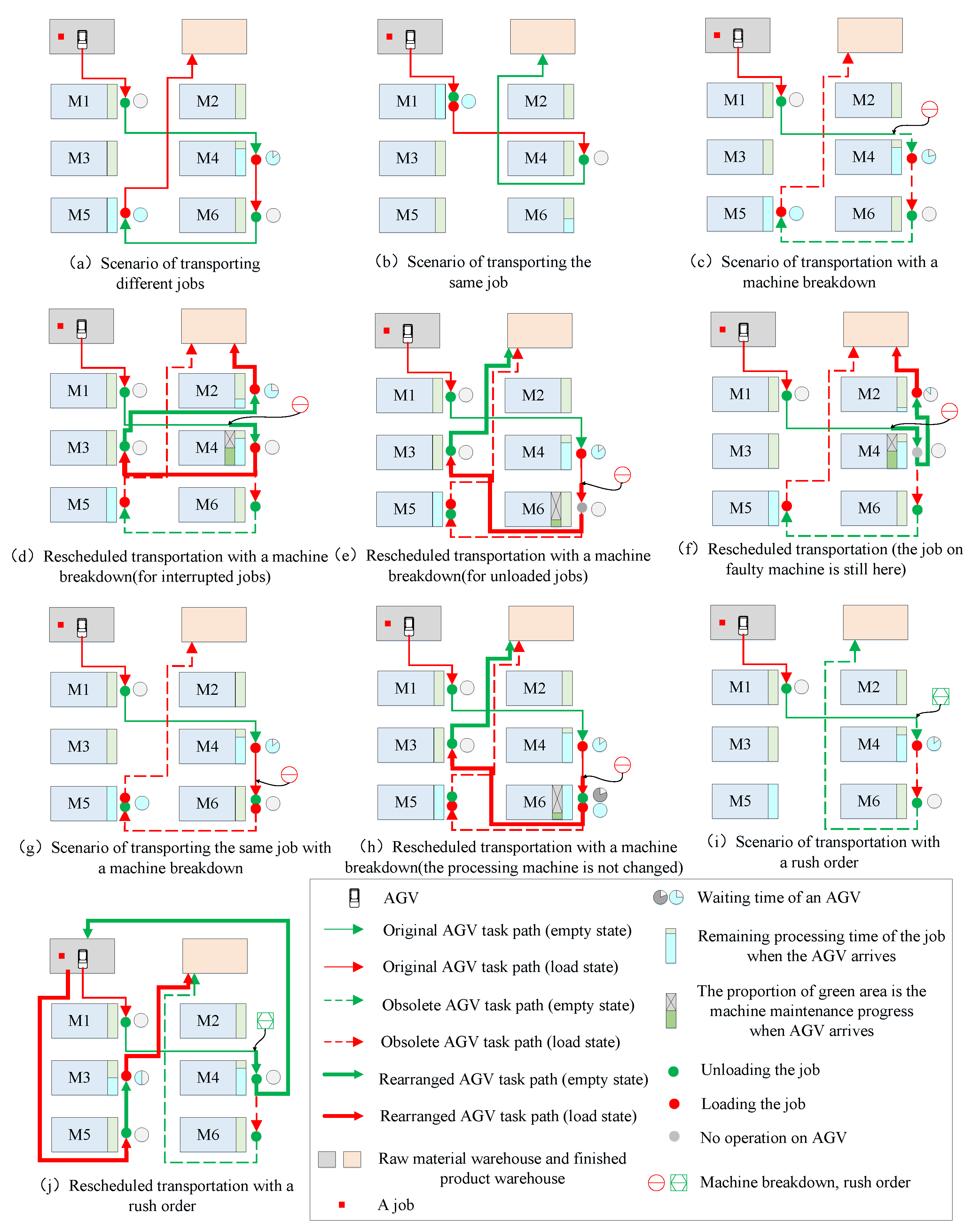
Figure 2.
Composition and relationship of problem elements.
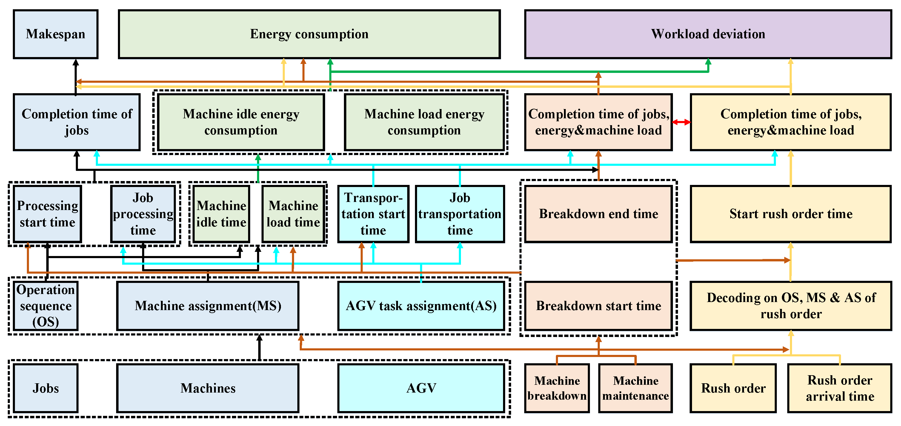
Figure 3.
Flowchart of the proposed approach for FJSP-AMBRO.

Figure 4.
Three-layer encoding mode.
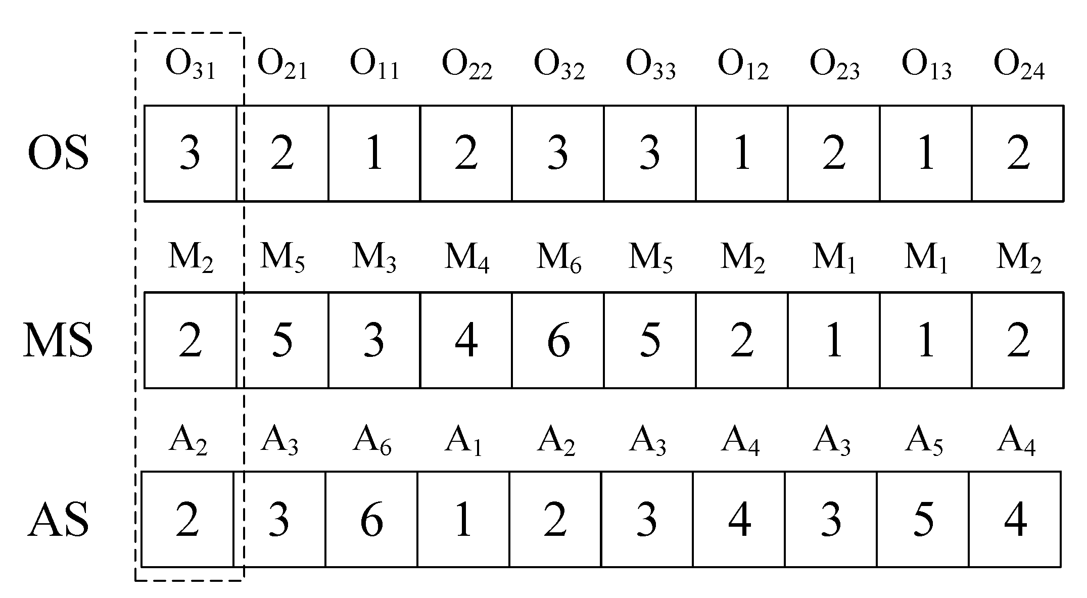
Figure 5.
POX crossover mode.

Figure 6.
Three mutations of OS.

Figure 7.
Critical path transformation.
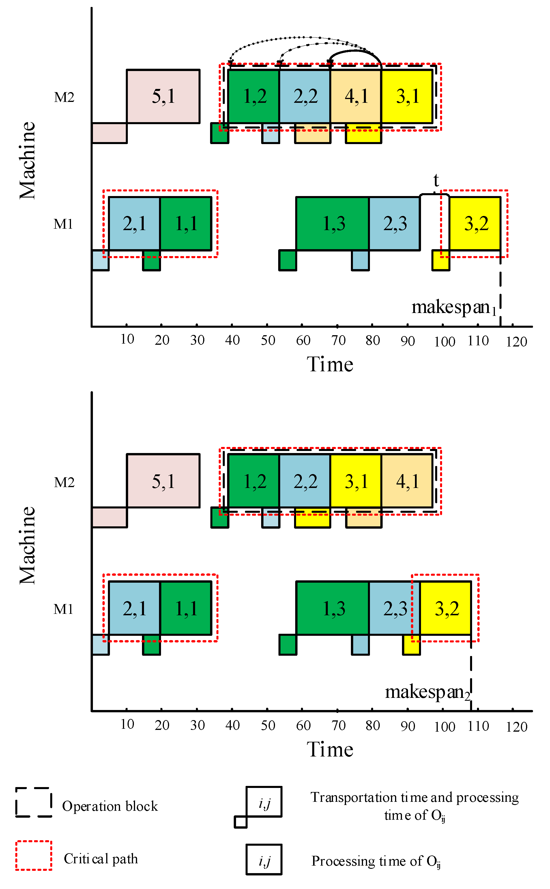
Figure 8.
The mean-main effect response diagram of IGD.

Figure 9.
Pareto fronts for Mk-01.

Figure 10.
Pareto fronts for Mk-05.
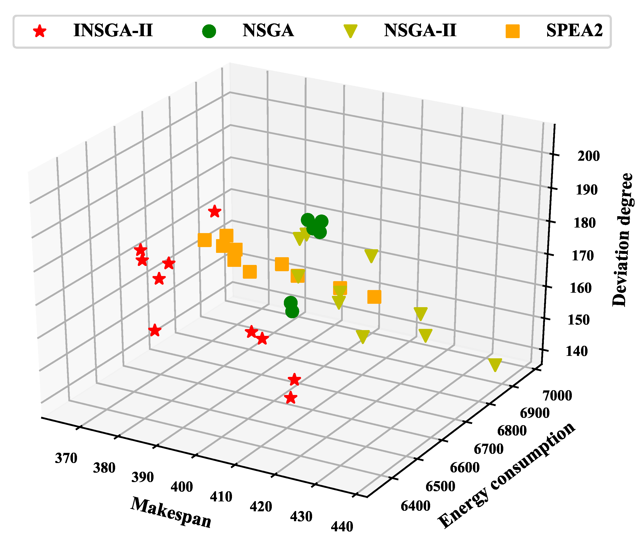
Figure 11.
Pareto fronts for Mk-10.

Figure 12.
Pareto fronts for Mk-15.


Table 1.
List of notations.
| Symbol | Meaning |
|---|---|
| n | Number of jobs for initial order |
| n* | Number of jobs for initial order and rush orders |
| m | Number of machines |
| g | Number of AGVs |
| i | Job index |
| j | Operation index |
| k | Machine index |
| s | AGV index |
| Operation number of job i | |
| The operation j of job i | |
| The processing time of on machine k | |
| The start time of on machine k | |
| The completion time of on machine k | |
| The earliest transportable time for transportation task from processing machine of to processing machine of by AGV s | |
| The arrival time of the transportation task from the processing machine of to the processing machine of by AGV s | |
| The time for the transportation task from the processing machine of to the processing machine of | |
| The start time of machine breakdown | |
| The available time after machine breakdown | |
| The completion time of job i | |
| Working power of machine k | |
| TE | Total energy consumption of all machines |
| M | A positive number large enough |
| Machine selection decision variable. If is processed on machine k, then ; otherwise | |
| Reschedule machine selection decision variable. If is processed on machine k after rescheduling, then ; otherwise | |
| Machine condition variables. If is the immediately preceding operation of on machine k, then ; otherwis | |
| AGV selection decision variable. If the transportation task from processing machine of to processing machine of is carried out by the AGV s, then ; otherwise | |
| AGV condition variable. If the transportation task of AGV s from processing machine of to processing machine of is earlier than that from to , then ; otherwise | |
| Machine state variable. If there is a breakdown on machine k, = 1; Otherwise, = 0 | |
| Job status variable. If is less than and is more than , =1; Otherwise, = 0 |
Table 2.
Parameters with corresponding levels.
| Factor | Levels | ||||
|---|---|---|---|---|---|
| 1 | 2 | 3 | 4 | 5 | |
| MaxIt1 | 200 | 300 | 400 | 500 | 600 |
| PC1 | 0.40 | 0.50 | 0.60 | 0.70 | 0.80 |
| PM1 | 0.01 | 0.05 | 0.10 | 0.15 | 0.20 |
| MaxIt2 | 200 | 300 | 400 | 500 | 600 |
| PC2 | 0.40 | 0.50 | 0.60 | 0.70 | 0.80 |
| PM2 | 0.01 | 0.05 | 0.10 | 0.15 | 0.20 |
Table 3.
Orthogonal test results.
| Parameter Combinations | Level | IGD | |||||
|---|---|---|---|---|---|---|---|
| MaxIt1 | PC1 | PM1 | MaxIt2 | PC2 | PM2 | ||
| 1 | 1 | 1 | 1 | 1 | 1 | 1 | 1166.25 |
| 2 | 1 | 2 | 2 | 2 | 2 | 2 | 1211.99 |
| 3 | 1 | 3 | 3 | 3 | 3 | 3 | 1042.18 |
| 4 | 1 | 4 | 4 | 4 | 4 | 4 | 1035.20 |
| 5 | 1 | 5 | 5 | 5 | 5 | 5 | 1019.37 |
| 6 | 2 | 1 | 2 | 3 | 4 | 5 | 1122.31 |
| 7 | 2 | 2 | 3 | 4 | 5 | 1 | 1071.06 |
| 8 | 2 | 3 | 4 | 5 | 1 | 2 | 1108.89 |
| 9 | 2 | 4 | 5 | 1 | 2 | 3 | 1396.53 |
| 10 | 2 | 5 | 1 | 2 | 3 | 4 | 1083.94 |
| 11 | 3 | 1 | 3 | 5 | 2 | 4 | 976.71 |
| 12 | 3 | 2 | 4 | 1 | 3 | 5 | 1150.72 |
| 13 | 3 | 3 | 5 | 2 | 4 | 1 | 1256.44 |
| 14 | 3 | 4 | 1 | 3 | 5 | 2 | 1277.04 |
| 15 | 3 | 5 | 2 | 4 | 1 | 3 | 1141.59 |
| 16 | 4 | 1 | 4 | 2 | 5 | 3 | 1120.62 |
| 17 | 4 | 2 | 5 | 3 | 1 | 4 | 938.70 |
| 18 | 4 | 3 | 1 | 4 | 2 | 5 | 972.39 |
| 19 | 4 | 4 | 2 | 5 | 3 | 1 | 1129.60 |
| 20 | 4 | 5 | 3 | 1 | 4 | 2 | 1404.60 |
| 21 | 5 | 1 | 5 | 4 | 3 | 2 | 1084.39 |
| 22 | 5 | 2 | 1 | 5 | 4 | 3 | 1157.46 |
| 23 | 5 | 3 | 2 | 1 | 5 | 4 | 1372.36 |
| 24 | 5 | 4 | 3 | 2 | 1 | 5 | 1013.42 |
| 25 | 5 | 5 | 4 | 3 | 2 | 1 | 1324.13 |
Table 4.
IGD&C value comparison of NSGA-II and .
| Problem | IGD | C | |||||
|---|---|---|---|---|---|---|---|
| NSGA-II | INSGA-II | C(NSGA-II, ) | C(, NSGA-II) | C(INSGA-II, ) | C(, INSGA-II) | ||
| Mk-01 | 10.69 | 10.56 | 10.52↓ | 0.10 | 0.50 | 0.13 | 0.48 |
| Mk-02 | 11.39 | 11.25 | 11.17↓ | 0.03 | 0.63 | 0.22 | 0.23 |
| Mk-03 | 64.75 | 63.37 | 63.10↓ | 0.00 | 0.60 | 0.17 | 0.29 |
| Mk-04 | 14.27 | 14.05 | 13.04↓ | 0.25 | 0.29 | 0.27 | 0.29 |
| Mk-05 | 48.01 | 47.07 | 46.80↓ | 0.20 | 0.33 | 0.25 | 0.28 |
| Mk-06 | 31.09 | 29.74 | 29.09↓ | 0.00 | 0.10 | 0.16 | 0.30 |
| Mk-07 | 26.68 | 26.55 | 26.45↓ | 0.00 | 0.57 | 0.19 | 0.29 |
| Mk-08 | 67.48 | 67.26 | 64.73↓ | 0.27 | 0.31 | 0.03 | 0.43 |
| Mk-09 | 141.63 | 140.25 | 139.42↓ | 0.20 | 0.57 | 0.16 | 0.50 |
| Mk-10 | 164.34 | 161.98 | 161.61↓ | 0.12 | 0.51 | 0.29 | 0.34 |
| Mk-11 | 207.63 | 205.44 | 204.66↓ | 0.15 | 0.29 | 0.26 | 0.36 |
| Mk-12 | 216.12 | 214.10 | 213.51↓ | 0.22 | 0.35 | 0.18 | 0.43 |
| Mk-13 | 226.51 | 221.10 | 219.06↓ | 0.15 | 0.36 | 0.26 | 0.42 |
| Mk-14 | 365.57 | 364.74 | 361.60↓ | 0.21 | 0.45 | 0.27 | 0.32 |
| Mk-15 | 336.60 | 331.41 | 327.76↓ | 0.33 | 0.39 | 0.13 | 0.43 |
Table 5.
IGD comparison of each algorithm.
| Problem | n/m | INSGA-II | NSGA | NSGA-II | SPEA2 |
|---|---|---|---|---|---|
| Mk-01 | 10/6 | 10.18 | 10.72 | 11.02 | 11.79 |
| Mk-02 | 10/6 | 12.49 | 12.59 | 13.27 | 11.96 |
| Mk-03 | 15/8 | 63.43 | 66.67 | 63.78 | 67.11 |
| Mk-04 | 15/8 | 11.48 | 13.08 | 12.03 | 12.42 |
| Mk-05 | 15/4 | 44.35 | 45.13 | 44.87 | 45.01 |
| Mk-06 | 10/15 | 28.88 | 30.88 | 29.64 | 33.50 |
| Mk-07 | 20/5 | 27.06 | 30.13 | 27.33 | 33.04 |
| Mk-08 | 20/10 | 64.70 | 65.33 | 64.29 | 64.83 |
| Mk-09 | 20/10 | 141.43 | 145.03 | 142.64 | 146.16 |
| Mk-10 | 20/15 | 162.46 | 167.04 | 163.34 | 165.02 |
| Mk-11 | 30/5 | 202.23 | 206.45 | 206.01 | 203.44 |
| Mk-12 | 30/10 | 209.62 | 217.41 | 215.39 | 211.60 |
| Mk-13 | 30/10 | 221.19 | 227.16 | 223.85 | 231.92 |
| Mk-14 | 30/15 | 363.32 | 368.55 | 365.66 | 368.33 |
| Mk-15 | 30/15 | 337.39 | 346.04 | 341.23 | 344.24 |
Table 6.
Comparison of the C-metric of each algorithm.
| Problem | C(INSGA-II, NSGA) | C(NSGA, INSGA-II) | C(INSGA-II, NSGA-II) | C(NSGA-II, INSGA-II) | C(INSGA-II, SPEA2) | C(SPEA2, INSGA-II) |
|---|---|---|---|---|---|---|
| Mk-01 | 0.48 | 0.11 | 0.30 | 0.21 | 0.34 | 0.20 |
| Mk-02 | 0.51 | 0.14 | 0.34 | 0.20 | 0.92 | 0.00 |
| Mk-03 | 0.42 | 0.12 | 0.35 | 0.17 | 0.58 | 0.04 |
| Mk-04 | 0.48 | 0.08 | 0.29 | 0.18 | 0.72 | 0.08 |
| Mk-05 | 0.30 | 0.08 | 0.31 | 0.18 | 0.44 | 0.03 |
| Mk-06 | 0.34 | 0.10 | 0.14 | 0.12 | 0.99 | 0.00 |
| Mk-07 | 0.54 | 0.07 | 0.35 | 0.26 | 0.84 | 0.00 |
| Mk-08 | 0.55 | 0.10 | 0.28 | 0.19 | 0.57 | 0.00 |
| Mk-09 | 0.65 | 0.05 | 0.25 | 0.19 | 0.83 | 0.01 |
| Mk-10 | 0.59 | 0.03 | 0.38 | 0.09 | 0.77 | 0.01 |
| Mk-11 | 0.41 | 0.18 | 0.17 | 0.17 | 0.32 | 0.02 |
| Mk-12 | 0.50 | 0.06 | 0.32 | 0.17 | 0.40 | 0.02 |
| Mk-13 | 0.70 | 0.05 | 0.25 | 0.16 | 0.89 | 0.00 |
| Mk-14 | 0.63 | 0.06 | 0.37 | 0.17 | 0.44 | 0.05 |
| Mk-15 | 0.63 | 0.09 | 0.30 | 0.07 | 0.80 | 0.00 |
Table 7.
Pair-wise t-test results of each two algorithms on IGD value (df = 14).
| Algorithm | Mean | Std. Deviation | Std. Error Mean | t | Sig. (2-tailed) |
|---|---|---|---|---|---|
| INSGA-II-NSGA | −3.46733 | 2.64179 | 0.68211 | −5.083 | 0.000 |
| INSGA-II-NSGA-II | −1.61067 | 1.71294 | 0.44228 | −3.642 | 0.003 |
| INSGA-II-SPEA2 | −3.34533 | 3.02869 | 0.78200 | −4.278 | 0.001 |
Disclaimer/Publisher’s Note: The statements, opinions and data contained in all publications are solely those of the individual author(s) and contributor(s) and not of MDPI and/or the editor(s). MDPI and/or the editor(s) disclaim responsibility for any injury to people or property resulting from any ideas, methods, instructions or products referred to in the content. |
© 2023 by the authors. Licensee MDPI, Basel, Switzerland. This article is an open access article distributed under the terms and conditions of the Creative Commons Attribution (CC BY) license (https://creativecommons.org/licenses/by/4.0/).
Share and Cite
MDPI and ACS Style
Zhang, H.; Qin, C.; Zhang, W.; Xu, Z.; Xu, G.; Gao, Z. Energy-Saving Scheduling for Flexible Job Shop Problem with AGV Transportation Considering Emergencies. Systems 2023, 11, 103. https://doi.org/10.3390/systems11020103
AMA Style
Zhang H, Qin C, Zhang W, Xu Z, Xu G, Gao Z. Energy-Saving Scheduling for Flexible Job Shop Problem with AGV Transportation Considering Emergencies. Systems. 2023; 11(2):103. https://doi.org/10.3390/systems11020103
Chicago/Turabian StyleZhang, Hongliang, Chaoqun Qin, Wenhui Zhang, Zhenxing Xu, Gongjie Xu, and Zhenhua Gao. 2023. "Energy-Saving Scheduling for Flexible Job Shop Problem with AGV Transportation Considering Emergencies" Systems 11, no. 2: 103. https://doi.org/10.3390/systems11020103
Note that from the first issue of 2016, this journal uses article numbers instead of page numbers. See further details here.