Assessing the Loss Given Default of Bank Loans Using the Hybrid Algorithms Multi-Stage Model

Abstract

The loss given default (LGD) is an important credit risk parameter in the regulatory system for financial institutions. Due to the complex structure of the LGD distribution, we propose a new approach, called the hybrid algorithms multi-stage (HMS) model, to construct a multi-stage LGD prediction model and test it on the US Small Business Administration (SBA)’s small business credit dataset. We then compare the model’s performance under four routes by different evaluation metrics. Finally, pertinent business information and macroeconomic features datasets are added for robustness validation. The results show that HMS performs well and stably for predicting LGD, confirming the superiority of the proposed hybrid unsupervised and supervised machine learning algorithm. Financial institutions can apply the approach to make default predictions based on other credit datasets.

1. Introduction

When financial institutions extend loans to borrowers, credit risk is a major issue, which refers to the risk of default and non-fulfilment of debt servicing obligations by the borrower [1,2,3]. One of the key drivers of credit risk is loss given default (LGD). LGD is the ratio of the amount of loss to a lender resulting from a borrower’s default to risk exposure. It is critical to understand potential losses for effective allocation of regulatory and economic capital and credit risk pricing. According to Article 107 (1) of the Capital Requirements Regulation (CRR), financial institutions should use either the Standardized Approach (SA) or the Internal Ratings-Based Approach (IRBA) when calculating their regulatory capital requirements for credit risk. When implementing advanced IRBA, internal models must be developed to estimate exposure at default (EAD), probability of default (PD), and LGD. EAD is the risk exposure that arises when a default occurs. PD is the probability that a borrower defaults on a loan within a given period. One of the primary objectives of IRBA is to achieve risk-adjusted capital requirements (see Basel Committee on Banking Supervision [4]). As shown by Gürtler and Hibbeln [5], accurate forecasts for LGD may generally provide a competitive advantage for the applying financial institution, and therefore, banks use a variety of methodologies to estimate it.

LGD is an important measure that banks need to estimate accurately for several reasons. First, LGD is critical to risk management in banks and other financial institutions. Understanding and measuring LGD can help financial institutions better assess and control their credit risk exposures, i.e., it can be used in conjunction with PD and EAD to estimate expected financial losses, so banks can more accurately measure potential credit losses and thus be well prepared for future defaults. Second, financial institutions can improve their overall risk modelling by better understanding and estimating LGD, thereby improving their ability to measure and manage credit risk. This is important for maintaining the stability of the financial system and preventing financial crises. Third, estimations of LGD and portfolio financial risk are an indispensable part of calculating the capital requirements for covering credit losses under extreme economic conditions [6,7,8]. Thus, reliable LGD prediction models play important roles in loss control and benefit maximization.

A key focus of LGD prediction models is how to accurately improve their predictive performance and whether they can improve credit risk assessment, capital measurement or risk management. LGD forecasting is challenging because LGD does not follow a normal distribution [9]. A large proportion of defaulted loans are either fully recovered or not recovered at all [10,11]. Considering the complicated nature of the LGD distribution, a multi-stage modelling framework seems to be more appealing. Many studies have proposed multi-stage models for LGD prediction [5,6,12,13,14]. Most of them use a single supervised algorithm to predict in a multi-stage model to achieve good prediction accuracy. However, they are deficient in several aspects: First, LGD prediction usually involves multiple factors and variables, and a single supervised model may have difficulty in capturing all these complexities. In addition, an over-reliance on a supervised algorithm can lead to overfitting problems [2,15]. Second, it is likely to encounter data imbalance in LGD prediction, i.e., unbalanced proportions of defaulted and non-defaulted samples. A single supervised model may not perform well under such a scenario. Third, the importance of interpreting model predictions is critical and a single supervised model may be less able to provide a clear explanation for the financial domain under consideration. To address the above problems, our idea is to use an efficient unsupervised algorithm as a high-level method in a multi-stage LGD model and propose a new approach called the hybrid algorithms multi-stage (HMS) model.

Another key focus of LGD prediction is to obtain real credit data, as customer credit data are confidential to most financial institutions and researchers do not have access to such data [15]. The US Small Business Administration (SBA) dataset has been extensively used for default risk research for many years [16]. One of the benefits of this dataset is that we can tap into some pertinent information about a firm (indirectly reflecting the features of the firm’s financial level such as its loans backed by real estate) and macroeconomic features to improve the prediction performance of the developed model. This is because if an entrepreneur borrows from a bank, their background can be understood indirectly through unobservable characteristics. A change in the macroeconomic environment can also lead to a sudden risk status change [17,18,19], especially in a recession when many firms are strapped for funds or resources. Small firms are more weakened in access to early external support and resources, and banks’ LGD may be further raised. But the drawback is the incompleteness of the data. Incompleteness means that some specific data fields are blank because some data may not have been collected from all borrowers, the data collection process may have been modified, or the borrowers may have neglected to submit some optional items when completing the form. However, such a “missing state” is worth mining and can be used to segment the dataset. It is widely believed that segmentation improves the performance of prediction models [15,20] We first consider some pertinent information about small businesses and then use HMS to explore whether using such information helps improve the performance of the LGD prediction model. From a management perspective, this approach is more accurate than the other methods, as it is not limited to sorting customers into prespecified categories [2].

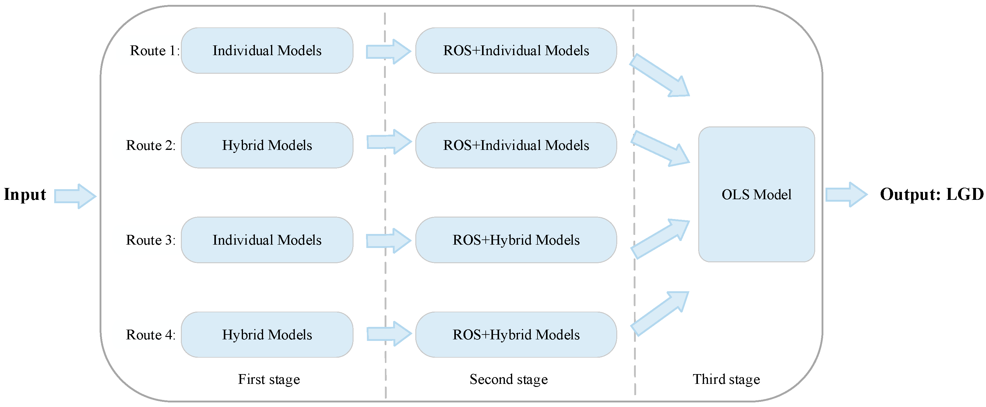
We use data from the SBA, which promotes and assists small business lending in the US credit markets to develop the HMS model for commercial banks possessing large amounts of data and being exposed to high default rates on commercial loans. We divide the borrowers’ LGD into three stages, resulting in three different data features for the dataset. Specifically, in the first stage, based on a binary feature dataset, we apply different unsupervised learning algorithms to cluster borrowers. We then apply different supervised learning algorithms to predict whether a customer will incur a loss. In the second stage, based on a binary feature and a sample imbalance dataset, we first perform Random Oversampling (ROS), which refers to balancing the class distribution by randomly replicating a small number of class samples to solve the class imbalance problem, and then apply a hybrid algorithm to predict whether a customer will incur a full loss. In the third stage, based on a continuous dataset, we apply a simple ordinary least squares (OLS) model to predict the partial loss degrees of the borrowers. Finally, we provide a comprehensive assessment of the borrowers’ LGD to help commercial banks make sound lending decisions. In addition, the dataset includes some information that may be relevant to firms and macroeconomic recession features as additional features for robustness validation. We show the main idea of HMS in Figure 1. To test the validity of HMS, we compare different integrated methods under four routes in a multi-stage LGD prediction model, as shown in Figure 2, whose prediction performance is measured by different metrics such as the mean absolute error (MAE), explained variance (EV), and mean squared error (MSE).

Our HMS model has important practical implications. First, the HMS model allows credit risk management to be broken down into multiple stages, each focusing on different risk factors and data. This granular risk management helps financial institutions better understand and manage their customers’ credit risk. Second, the HMS model provides more accurate estimates of credit risk, which improves the determination of capital requirements. This helps financial institutions to ensure that sufficient capital is available to meet potential credit losses. Finally, financial regulators often require financial institutions to adequately assess and manage their credit risk, and the use of HMS models helps financial institutions meet regulatory requirements by providing more transparent and interpretable credit risk estimates.

We contribute to the literature in the following ways. First, by adding unsupervised learning algorithms, our approach can help mitigate the overfitting of outputs in multi-stage LGD models, which is typically a problem associated with the implementation of supervised learning algorithms. Unsupervised learning algorithms help discover the underlying structures and patterns in the data, thus improving the generalization of the model and reducing the risk of overfitting. Second, we construct a new HMS model for LGD forecasting for commercial banks in the SBA dataset. The HMS model combines multiple algorithms, including supervised and unsupervised learning algorithms, to improve the performance and robustness of the model. Finally, we test the importance of potential credit risk and macroeconomic recession characteristics for LGD forecasting, which can help financial institutions detect and respond to possible credit risk upturns in a timelier manner. This experiment is crucial for gaining insights into the credit risks of borrowers with different LGD, helping financial institutions develop more effective risk management strategies.

We organize the rest of the paper as follows: Section 2 provides a literature review of research on LGD. Section 3 discusses the data pre-processing approach and research methodology. Section 4 presents the experimental results, robustness validation analysis, and discussion of the research findings and their practical implications. Section 5 concludes the paper and suggests topics for future research.

2. Literature Review on LGD

2.1. Theoretical Development of LGD

The Basel Capital Accord aims to better integrate regulatory capital with the underlying risks in a bank’s credit portfolio. Banks have the flexibility to calculate their credit risk capital through two distinct methods: a modified standardized approach rooted in the original 1988 capital agreement and two variations based on the Internal Ratings-Based (IRB) approach, which allows banks to develop and use their own internal risk ratings. The internal ratings methodology relies on four main parameters for assessing credit risk: EAD, PD, LGD and M. M is Maturity, which refers to the deadline for repayment of a loan. For a particular maturity, these parameters are used to compute two forms of expected loss (EL): expected loss as an amount (the formula is EL = EAD × PD × LGD) and expected loss as a percentage of exposure at default (the formula is EL% = PD × LGD).

Several decades ago, academic research and banking practice primarily emphasized predicting PD. However, in recent years, considerable attention has shifted towards modelling LGD. The main reason for this is that the Basel II/III framework requires banks to give their own estimates of LGD when using IRBA methods for businesses or internal rating methods for retail exposures. Apart from meeting regulatory demands, precise LGD predictions play a crucial role in making risk-informed decisions. For example, they help determine risk-adjusted loan pricing, calculate economic capital, and price assets such as asset-backed securities or credit derivatives. [21].

The relevant literature on LGDs has different streams. Some research endeavours aim to gauge the LGD distribution for credit portfolio modelling [22,23]. Meanwhile, others focus on examining the factors that impact individual LGD. In addition, certain studies explore the relation between PD and LGD [24,25,26]. While a large of the literature consists of empirical investigations into corporate bonds, there is relatively less emphasis on bank loans, primarily due to constraints related to data availability. The primary objective of this paper is to enhance the prediction of LGDs for bank loans. We conduct a theoretical analysis of various challenges associated with forecasting LGDs and provide actionable recommendations to achieve consistent estimates with robust predictive capability.

2.2. LGD Modelling

A wide range of LGD modelling techniques have been applied in the literature in the past. Benchmark regression models include simple linear regression and fractional response regression, where a logit link function is used to convert linear combinations to fractional values bounded by 0 and 1 [27]. A more complicated regression model is the beta transformation for accommodating irregular LGD distributions. However, machine learning (ML) techniques, such as decision tree (DT) and support vector regression, are more effective and competitive than the traditional parametric regression models [28,29,30,31]. In recent studies, random forest (RF) has been found to outperform other techniques in predicting LGD [32,33,34,35].

Unsupervised ML algorithms usually include clustering algorithms, which are important data mining techniques that cluster samples into groups of similar objects rather than giving direct predictions. As such, these unsupervised ML algorithms are often used as complementary tools to supervised ML algorithms. Some studies have concentrated on clustering support vector machine (SVM) models using unsupervised ML algorithms (e.g., K-means and self-organized maps (SOMs)) [36,37,38,39]. On the other hand, unsupervised ML algorithms, such as SOMs, that can be used for prediction have been proposed, but relatively few applications have been reported in the field of LGD evaluation [40,41].

Many studies have proposed multi-stage models for LGD prediction [5,6,12,13,42]. In the earliest studies, Lucas [13] proposes a two-stage model to analyse mortgage-related LGD, i.e., dividing the loan according to whether or not it is recovered and calculating the loss in case of recovery. A scorecard is constructed to calculate the likelihood of repossession, followed by the utilization of a model to estimate the “haircut”, which represents the proportion of the estimated house sale value that is realized during the actual sale. However, the scorecard is not applicable to certain credit risk problems with a high degree of complexity. Gürtler and Hibbeln [5] classify defaults into two types (recovery/write-off) an d model LGD through a two-step modelling approach by taking into account length bias sampling, different loan characteristics for default end types, and different information sets for default status, which provides a significant improvement in predictive power compared to direct regression methods. However, they do not fully consider the potential impact of macroeconomic recession or volatility on LGD forecasts and may be somewhat biased. Bellotti and Crook [6] propose a multi-stage model for LGD prediction (consisting of two LR classifications and an OLS regression) and find that it is important to incorporate macroeconomic features into the developed model. But the class imbalance problem in LR classification prediction has not been solved, and the overall model prediction ability needs to be improved. Tanoue et al. [14] analyse the factors influencing LGD using Japanese bank loan data and develop a multi-stage model for predicting the LGD and expected loss (EL). The shortcoming of their study is that, due to data deficiencies, only credit score and different types of collateral quotas are considered, and more potential factors are not fully explored. Li et al. [12] added the disclosure of post default information to build two models, namely the hierarchical (two-stage) and hybrid models, to predict LGD separately. Most techniques use supervised algorithms as advanced learners in multiple stages to achieve good prediction accuracy. However, first they are dealing with the complexity of the data, such as multidimensional credit information. Traditional supervised learning algorithms may not be able to adequately capture these complexities, resulting in a decrease in model performance. Second, facing the sample imbalance problem, supervised learning algorithms may tend to favour the prediction of categories with more samples over those with fewer samples, leading to poorer model performance in predicting defaults. Finally, the overfitting problem caused by over-reliance on supervised algorithms is less able to generalize new data. [2,15] Combining the above problems, we propose the HMS model and fully consider some potential factors with macroeconomic aspects to predict LGD.

3. Methodology

In this section we present our proposed methodology in four aspects: credit dataset description, data pre-processing techniques, model framework and algorithms, and model performance evaluation. The overall process of the HMS model is shown in Figure 3.

3.1. Credit Dataset

The data for this study come from the large and rich US SBA credit dataset1. We focus on the data on the loan default risk based on the payment date (Disbursement_Date) for three large banks over the period January 2003 to June 2013. The dataset has a total of 89,903 samples, including 39,943 defaults (bad borrowers) and 49,960 non-defaults (good borrowers).

Table 1. Description of the credit dataset.

Dataset	Total	Non-Defaults	Defaults	Defaults Ratio
Bank 1	51,827	31,778	20,049	38.68%
Bank 2	20,433	11,526	8907	43.59%
Bank 3	17,643	6656	10,987	62.27%

presents the sample size, number of defaults, and default rates for the three large banks in the dataset. We find that each large bank has a high rate of small business defaults, the highest being 62.27%, which makes the bank vulnerable to financial crises, so it is important to predict the expected losses of small businesses. There are three types of data for the independent variables, including borrowers’ information, business financial projection information, and macroeconomic features, as shown in

Table 2. Descriptive statistics of the variables.

	Bank 1				Bank 2				Bank 3
Variables	Mean	SD	Min	Max	Mean	SD	Min	Max	Mean	SD	Min	Max
NoEmp	4.948	7.044	0.000	100	5.825	7.477	0.000	92	3.452	5.230	0.000	100
UrbanRural	0.925	0.263	0.000	1.000	0.860	0.347	0.000	1.000	0.932	0.252	0.000	1.000
NewExist	0.764	0.424	0.000	1.000	0.964	0.186	0.000	1.000	0.649	0.477	0.000	1.000
Createjob	0.651	2.159	0.000	50	1.041	2.288	0.000	50	1.859	3.108	0.000	50
Protion	0.503	0.030	0.350	0.955	0.513	0.065	0.500	0.900	0.811	0.107	0.200	1.000
isFranchise	0.010	0.102	0.000	1.000	0.009	0.094	0.000	1.000	0.007	0.084	0.000	1.000
Retainedjob	4.554	6.894	0.000	100	4.943	7.114	0.000	90	3.362	5.190	0.000	100
DisbursementGross	52,986	73,230	4000	2,293,500	5.825	7.477	0.000	92	67,338	223,261	4729	4,200,000
Real_Estate	0.001	0.034	0.000	1.000	0.000	0.007	0.000	1.000	0.024	0.154	0.000	1.000
Recession	0.030	0.169	0.000	1.000	0.018	0.131	0.000	1.000	0.146	0.353	0.000	1.000
LGD	0.329	0.436	0.000	1.000	0.306	0.383	0.000	1.000	0.470	0.400	0.000	1.000

Note: The borrower information includes: NoEmp: number of employees; UrbanRural: region type (urban is 1 and rural is 0); NewExist: a dummy variable that is 1 for an existing business when the business is more than two years old, otherwise 0 for a new business; Createjob: number of new jobs; Protion: percentage of loans guaranteed by the SBA per small/start-up business; isFranchise: a dummy variable that indicates whether the business has a franchise (0 for independent business and 1 for franchise); Retainedjob: number of jobs retained. The business financial projection information includes: DisbursementGross: total payments for small/start-up businesses and Real_Estate: indicating whether the firm has a real estate loan or not (1 if the term of the loan is more than 20 years; otherwise, 0). The macroeconomic feature is Recession (1 if the loan is active during the Great Recession between December 2007 and June 2009; otherwise, 0).

. The average value of LGD of 0.329 indicates that the expected financial loss in each default scenario averages 32.9%.

3.2. Data Pre-Processing

During the data pre-processing phase, we address some of the issues present in the data as follows. (i) We empirically handle the null points by removing the characteristics that are not filled in by more than 90% of the borrowers and replacing the remaining null-point characteristics with the mean, median, or plurality of their variables. (ii) We use the Upper and Lower Quartile Method, which is a statistical method commonly used for outlier treatment. The upper quartile (usually the 95% quartile) and the lower quartile (usually the 5% quartile) of the data are used to identify and handle outliers. Due to the small number of outlier observations, we directly remove the outliers. (iii) To treat the continuous variables, we standardise the eigenvalues by the Z-value, and the processed data conform to the standard normal distribution. (iv) To process the categorical variables, we create dummy variables to validate their behaviours and determine their importance to the model. (v) We test for multicollinearity using the variance inflation factor (VIF). We find no highly correlated features in the main dataset (all the VIFs are less than 5), so we do not remove any variables. (vi) We conduct correlation analysis, whereby we remove features from the final dataset when there are high correlations (above 90%) between them.

3.3. Model Framework

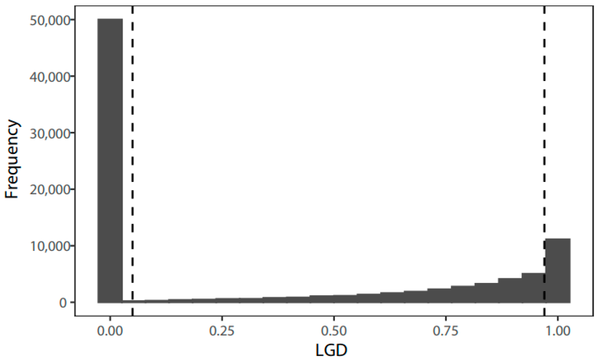
Since borrowers with recovered loans typically do not incur losses, we assume that their LGDs is 0. As shown in Figure 4, the LGD distribution peaks at the boundaries of 0 and 1, while the middle part of (0, 1) shows a steady upward trend. We might expect the segmentation stage to model LGD effectively, so we consider LGD prediction as a combination of two classification problems and one regression problem. This is because there may be special cases where the borrowers either repay the loan in full, do not repay the loan at all, and only partially repay the loan. We first divide the multi-stage LGD model into a first stage binary model with incurred loss (LGD > 0) and without incurred loss (LGD = 0), then a second stage binary model with partial loss (0 < LGD < 1) and full loss (LGD = 1) from incurred loss, and finally a third stage with continuous type of partial loss.

Specifically, for the binary classification problem of whether a loss occurs in the first stage (LGD = 0 with 49,960 and LGD > 0 with 39,943, a ratio close to 1:1), we perform predictions and comparisons between the hybrid and individual algorithms. For the second stage of the binary classification problem of whether full loss occurs (0 < LGD < 1 with 33,720 and LGD = 1 with 6223, a ratio of more than 5:1), because of sample imbalance, we first re-sample the data to make the ratio close. We then perform predictions and comparisons between the hybrid and individual algorithms. For the third stage of predicting the continuous partial loss problem, as shown in Figure 4, the LGDs lie in the middle (0,1) range and are largely linear, except for the 0 and 1 boundary points, so we use simple OLS regression for prediction. In summary, based on the three sub-models in Figure 3, the LGD of account $i$ is calculated as the expected value of $\left(1-p_{0i}\right)\left\{p_{1i}+\left(1-p_{1i}\right)L_i\right\}$, where $p_{0i}$ is the probability that LGD = 0 for account $i$ estimated by the first stage, $p_{1i}$ is the probability that LGD = 1 as estimated by the second stage, and $L_i$ is the OLS estimate of the third stage. The losses are assumed to be fractional and are calculated from the regression model.

3.4. Related Algorithms

The new HMS model includes both supervised and unsupervised algorithms and adopts the random over-sampling (ROS) approach based on the class imbalance that occurs in the data. Furthermore, we measure the predictive performance of the model by using different metrics. We describe the different algorithms and metrics below.

3.4.1. Unsupervised ML

K-means: K-means is a simple and effective unsupervised learning algorithm to ring customers into k pre-defined clusters [43]. The k-means model contains only one main parameter, namely the number of clusters k. We use the K-means method, which clusters the given samples according to the presence condition (missing or not), to divide the dataset into subsets and construct supervised ML models based on these subsets. The steps of this optimisation algorithm can be found in Machado and Karray [2].

Self-organizing map (SOM): SOM is an unsupervised neural network introduced by Kohonen [44]. SOM is essentially a neural network with only an input layer and a competing layer (output layer), which self-organizes and self-adaptively changes the network parameters and structure by automatically searching for inherent regularity and essential properties in the input sample. SOM is also a dimensionality reduction algorithm, as it maps high-dimensional inputs to a low-dimensional discretized representation while retaining the underlying structure of its input space.

3.4.2. Supervised ML

Ordinary least squares (OLS) regression: OLS regression is the simplest linear regression model for estimating the linear least squares values of unknown parameters. OLS selects the parameters as a linear function of a set of explanatory variables by the principle of least squares, i.e., minimising the sum of squares of the residuals between the dependent variable (the value of the predicted variable) and the predictor variables observed in a given data set. This is one of the most basic forms of LGD regression analysis [45,46].

Logistic regression (LR): LR is one of the classic algorithms in ML and is still one of the most basic and popular algorithms for classification problems due to its simplicity, effectiveness, parallelizability and interpretability. It is used to solve binary classification problems (default and non-default are the two categories in this work) and regression problems. LR can be a benchmark for the credit scoring problem [47].

Decision tree (DT): DT is a predictive (decision) model in ML that represents a mapping relationship between target attributes and target values. The DT classification model is a tree structure that describes the classification of instances. The DT model categorises input samples by ranking them in a tree and then assigning them to the most appropriate leaf nodes (class labels). In a DT diagram, each node represents a feature of the sample and each branch represents a possible value of that feature [15].

Random forest (RF): RF refers to a classifier that uses multiple trees to train and predict samples. The specific process is as follows: (i) randomly select a subset of the training data and train a decision tree model on it. (ii) Repeat the above process several times for the entire dataset, choosing a different subset of data each time and training multiple decision tree models. (iii) Combine the predictions from multiple decision tree models to produce a final prediction. RF is flexible and easily works with ML algorithms, providing great results in most cases, even without hyper-parameter tuning [34].

Gradient boosting decision tree (GBDT): GBDT is an iterative DT algorithm, also known as the multiple additive regression tree (MART) method. It works by constructing a weak set of learners (trees) and accumulating the results of multiple DT as the final prediction output. The algorithm combines DTs with integration ideas in an effective way. GBDT is applicable to a wide range of regression, binary classification, and multi-classification problems, and is a very powerful model [48].

eXtreme gradient boosting (XGBoost): XGBoost is an integrated ML algorithm based on DTs that uses GBoost as a framework and is developed from the GBDT method. Its main objective is to enhance the speed and efficiency of the model operations. The learning optimisation process uses an additive model with a forward stepwise algorithm. XGBoost not only adds a regular term but also supports row sampling to prevent overfitting. According to previous studies, XGBoost can obtain better results in the shortest time with fewer computing resources [49].

Multilayer perceptron (MLP): MLP is a convergent structured artificial neural network. The MLP neural network is fully connected between its different layers and it is not restricted to a specific number of hidden layers. The number of hidden layers can be adapted to meet application needs. During the optimization process (parameter solving), most neural networks are trained by error BackPropagation, i.e., the BP algorithm. MLP has great recognition rates and quick classification speeds [11].

Light gradient boosting machine (LightGBM): It is a new enhancement framework developed by Microsoft using a histogram-based DT algorithm. The basic idea is to first discretise the continuous floating-point eigenvalues and construct a histogram. While traversing the data, the histogram accumulates statistics based on the indices of the discrete values. After traversing the data once, the histogram accumulates the required statistics. Then, traversing the histogram finds the optimal segmentation point based on the discrete values of the histogram. LightGBM significantly outperforms the actual credit scoring models of banks [50].

3.4.3. Class Imbalance Handling Techniques

Data imbalance, i.e., the presence of only a few classes in the dataset, is the main challenge during model training. Data imbalance causes the model to try to pick up most classes and leads to skewed predictions. To tackle the data imbalance problem, we adopt the ROS technique, which effectively overcomes the problem of missing important categorical information. ROS works by randomly sampling a small number of classes and replicating them multiple times, thus increasing the number of classes and balancing the class distribution in the training set. Classification performance is slightly improved with ROS [51].

3.4.4. Performance Evaluation Metrics

In the first- and second-stage classification models, precision, recall, F1, the area under the curve (AUC), and accuracy (ACC) are the five most common validation metrics. In the final LGD regression model, MSE, root mean square error (RMSE), EV, MAE, and R-squared ($R^2$) are the five commonly used validation metrics. Their relevant descriptions are shown in

Table 3. Performance evaluation metrics.

Type	Measure	Description
Classification	AUC	The area enclosed with the coordinate axis under the Receiver Operating Characteristic (ROC) curve2.
	Accuracy	The proportion of correctly classified samples.
	Precision	The proportion of the truly classified samples to the total number of samples assigned to that class for a class.
	Recall	The proportion of true classified samples over the total of samples that belong to that class for a class.
	F1-score	This metric combines precision and recall by harmonizing averages and penalizes extreme values.
Regression	MSE	Square of the difference between the true value and predicted value, which is then summed and averaged.
	RMSE	MSE’s open square root.
	EV	The variance score of the explanatory regression model, which takes values in the range [0, 1].
	MAE	Average of the absolute errors.
	$R^2$	Coefficient of determination. It is usually between 0 and 1 and reflects how accurately the model fits the data.

.

3.4.5. Shapley Additive Explanations (SHAP)

SHAP is an additivity interpretation model inspired by Shapley value, commonly used to interpret machine learning models [52]. For each prediction sample, the model produces a prediction value and the SHAP value is the value assigned to each feature in that sample. Assuming that the $i$-th sample is $x_i$, the $j$-th feature of the $i$-th sample is $x_{i,j}$, the model’s predicted value for the $i$-th sample is $y_i$, and the baseline for the entire model (usually the mean of the target variable across all the samples) is $y_{base}$, then the SHAP value obeys the following equation.

$$y_i=y_{base}+f\left(x_{i,1}\right)+f\left(x_{i,2}\right)+\dots +f\left(x_{i,k}\right)$$

where $f\left(x_{i,1}\right)$ is the SHAP value for $x_{i,j}$. Intuitively, $f\left(x_{i,1}\right)$ is the contribution value of the $i$-th sample’s 1st feature to the final prediction value $y_i$. When $f\left(x_{i,1}\right)>0$, it means that the feature improves the prediction value and has a positive effect; otherwise, it means that the feature makes the prediction value lower and has a negative effect. SHAP can take the mean of the absolute values of how much a feature affects the target variable as the importance of that feature.

4. Experimental Results and Discussion

This section tests the HMS model on the SBA credit dataset. Specifically, we explore the data space of the SBA credit dataset, which contains cluster distribution mappings for default risk (loss and no loss) and for default loss (partial loss and full loss) in Section 4.1. Section 4.2 presents the modelling results for predicting whether a loss occurs in the first stage and shows the classification performance of the different models. Section 4.3 presents the modelling results in predicting whether a firm incurs a full loss. Section 4.4 presents the overall LGD prediction results. Section 4.5 presents the robustness tests. Finally, Section 4.6 provides a discussion.

4.1. Dataset Space

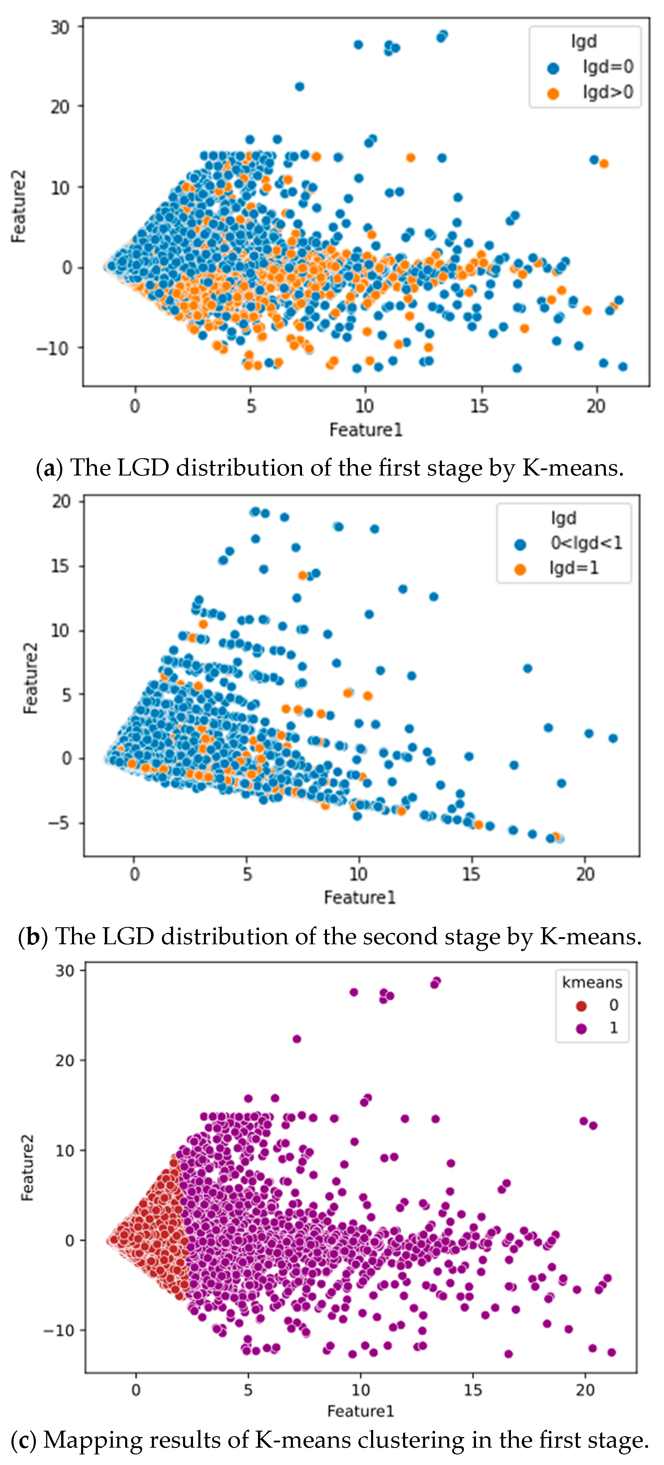
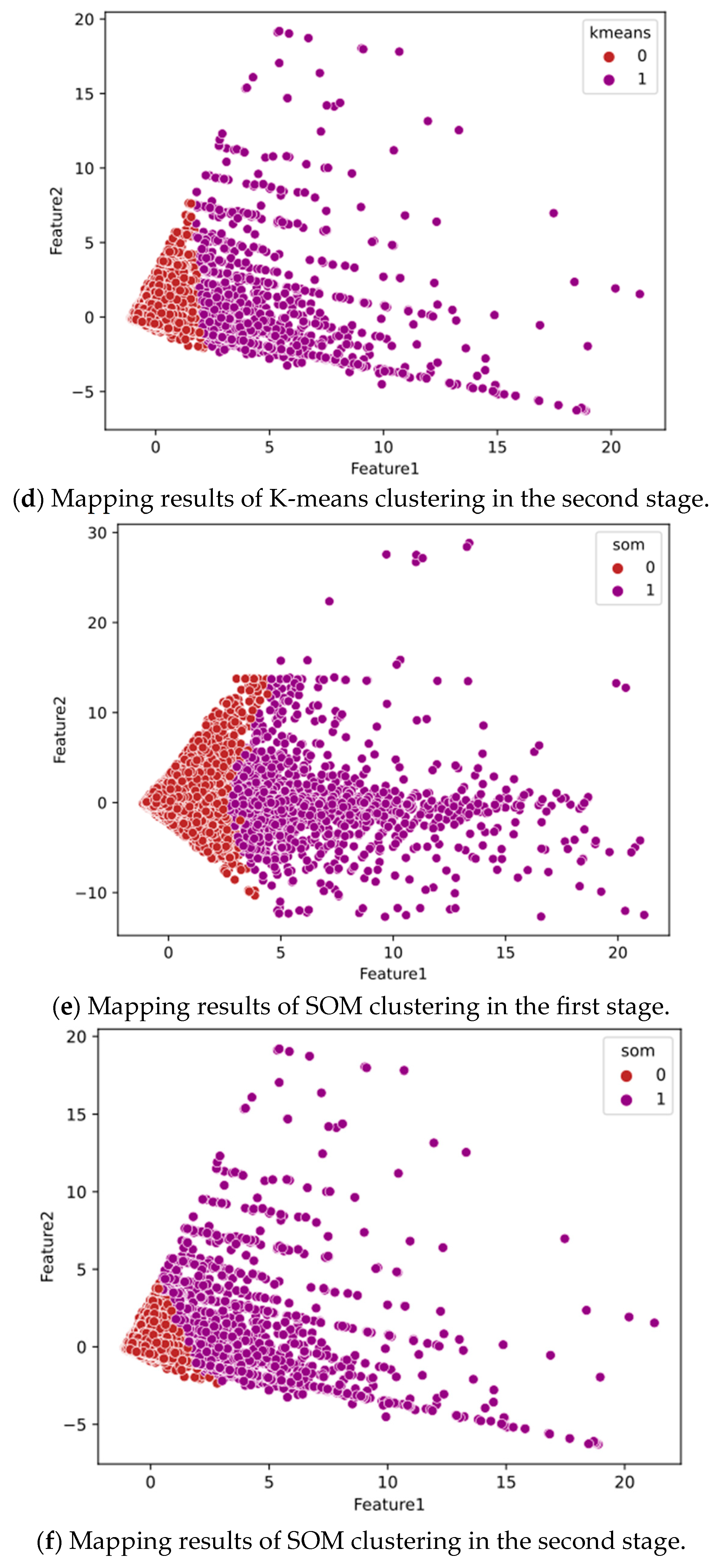
We explore the dataset space from the perspective of data existence conditions before building a multi-stage LGD model. For the first-stage samples, LGD = 0 is set to ‘0’ and LGD > 0 is set to ‘1’. For the second-stage samples, $LG{D}_{0<LGD<1}$ is set to ‘0’ and LGD = 1 is set to ‘1’. Then, we use K-means to cluster these two classes of LGD labelled ‘0’ and ‘1’ to obtain the distributions of LGD in Figure 5a and Figure 5b, respectively. The K-means clustering groups the first- and second-stage samples into two classes and the results are shown in Figure 5c and Figure 5d, respectively. SOM clustering also divides the first- and second-stage samples into two classes and the results are shown in Figure 5e and Figure 5f, respectively.

In the first stage of classification, the proportions of ‘0’ and ‘1’ samples in the LGD in Figure 5a distribute evenly. In Figure 5c,e, after classification by K-means and SOM, the binary classification ratio of the two categories becomes relatively balanced and the performance of the classifiers is not greatly affected, so we directly adopt the process of clustering before classification in the first stage.

In the second stage of classification, the number of ‘0’ samples for LGD are much larger than the number of ‘1’ samples in Figure 5b, with a significant difference between the two proportions. In addition, after performing K-means and SOM classification, the proportions of samples in Figure 5d,f after being classified into the two categories differ greatly, and the classifier fails to operate. This explains the necessity for ROS sampling in the second stage to balance the sample proportions and then clustering before classification.

4.2. Performance Evaluation of First-Stage Classification

To more accurately predict the probability of whether a loss occurs, we build individual and hybrid models separately in the first stage, and the results are shown in

Table 4. Performance of first-stage classification.

Clustering		Model	ACC	Precision	Recall	F1	AUC
Individual Models	no clustering	LR	0.6025	0.6355	0.2556	0.3645	0.5731
		DT	0.5958	0.5573	0.4570	0.5022	0.5947
		RF	0.5999	0.5605	0.4775	0.5157	0.6180
		GBDT	0.6295	0.6269	0.4186	0.5020	0.6694
		XGBoost	0.6274	0.6157	0.4387	0.5123	0.6697
		MLP	0.6265	0.6120	0.4449	0.5152	0.6641
		LightGBM	0.6298	0.6201	0.4389	0.5140	0.6718
K-means	clstering 1	LR	0.6052	0.6348	0.284	0.3925	0.6077
		DT	0.5968	0.5609	0.4691	0.5110	0.5936
		RF	0.6003	0.5623	0.4948	0.5264	0.6193
		GBDT	0.6331	0.6316	0.4389	0.5179	0.6743
		XGBoost	0.6338	0.6275	0.4539	0.5268	0.6744
		MLP	0.6304	0.6224	0.4493	0.5219	0.6699
		LightGBM	0.6341	0.6265	0.4585	0.5295	0.6773
	clustering 2	LR	0.6404	0.6386	0.1045	0.1797	0.6161
		DT	0.5788	0.4375	0.4142	0.4255	0.5580
		RF	0.5958	0.4561	0.3787	0.4138	0.5913
		GBDT	0.6263	0.5137	0.1479	0.2297	0.6157
		XGBoost	0.5854	0.4358	0.3412	0.3827	0.5902
		MLP	0.6397	0.641	0.0986	0.1709	0.6199
		LightGBM	0.6018	0.4589	0.3195	0.3767	0.6055
SOM	clustering 1	LR	0.6046	0.6403	0.2711	0.381	0.5982
		DT	0.5931	0.5563	0.4605	0.5039	0.5854
		RF	0.5989	0.5619	0.4816	0.5187	0.6135
		GBDT	0.6296	0.6233	0.4416	0.5169	0.6691
		XGBoost	0.6274	0.6153	0.4528	0.5217	0.6699
		MLP	0.6254	0.6065	0.4701	0.5297	0.6633
		LightGBM	0.6313	0.6228	0.4522	0.524	0.6718
	clustering 2	LR	0.6294	0.5714	0.1265	0.2072	0.5911
		DT	0.5866	0.4571	0.4282	0.4422	0.5657
		RF	0.5866	0.4545	0.4015	0.4264	0.5828
		GBDT	0.6145	0.4886	0.1557	0.2362	0.5967
		XGBoost	0.5931	0.4558	0.326	0.3801	0.5917
		MLP	0.6238	0.5321	0.1411	0.2231	0.5895
		LightGBM	0.6071	0.4804	0.3285	0.3902	0.5998

. Table 4 summarises the results of the model based on the test set of the SBA credit dataset, in terms of the ACC, AUC, F1, precision, and recall metrics. We use seven base learners (LR, DT, RF, GBDT, XGBoost, MLP, and LightGBM) to construct a single model and use the results as a baseline group (control group). Next, we use a hybrid ML model combining K-means and SOM with seven supervised learners for prediction, whose results serve as the experimental group. The purpose is to explore whether the application of unsupervised clustering on the dataset helps improve the accuracy of the first-stage classification predictions. Since these evaluation metrics describe the performance of the model in different ways, and no classifier outperforms the others in all the metrics, we focus on the use of AUC to evaluate the model because it considers the confusion matrix more comprehensively than the other metrics; it more effectively reflects the performance achieved by the model on the unbalanced dataset.

We can conclude the following based on AUC: First, the LightGBM model is best among all the individual models in Table 4, with AUC (0.6718) and ACC (0.6298) being the highest. Second, in the results of the supervised models built based on K-means and SOM clustering subsets, the models in clustering 1 (GBDT, XGBoost, and LightGBM in clustering 1) outperform the models built by the base learner in AUC values. The clustering approach provides the greatest improvement to the LR model, with a 7.5% improvement of AUC for K-means clustering 2. Among all the hybrid models, LightGBM based on K-means clustering 1 has the best performance with an AUC of 0.6773, which outperforms all the individual models. From the above results, we observe that the clustering method proposed on the SBA credit dataset does help improve the performance of the individual models.

Next, we perform an interpretability analysis based on the above optimal prediction model for the first stage of predicting whether a small business incurs a loss. We use SHAP to assess the feature importance of the model in the first stage, as shown in Figure 6. We find that the top two ranked features are NoEmp and DisbursementGross (total disbursements by small businesses), with mean absolute SHAP values of 0.2999 and 0.2585, respectively. Next are the percentage of loans guaranteed by the SBA for small businesses Portion (0.0913), the number of remaining jobs Retainedjob (0.0876), and economic recession Recession (0.0458). This indicates that the number of employees is a very important feature in the first stage of forecasting. Specifically, NoEmp has a greater impact on predicting whether a firm incurs a loss or not. Similarly, DisbursementGross is recognised as an important characteristic that has a significant impact on predicting whether a firm incurs a loss or not. This may indicate that the amount of payment by the firm plays an important role in the prediction. Additionally, Portion, Retainedjob and Recession correlate to some extent with whether a business incurs a loss. For banks, it is important to understand which characteristics are most important for a business’s credit assessment, which can help them to better develop a loan approval strategy. In this case, they may pay more attention to key features such as NoEmp and DisbursementGross to estimate the borrower’s credit risk more accurately.

4.3. Performance Evaluation of the Second-Stage Classification

To more accurately predict the probability of whether a full loss occurs, we apply the ROS technique to our model, which solves the problem of data imbalance. We then build individual and hybrid models in the second stage, and the results are shown in

Table 5. Performance of second-stage classification.

Clustering		Model	ACC	Precision	Recall	F1	AUC
ROS + Individual Models	no clustering	LR	0.6597	0.6059	0.9304	0.7339	0.7105
		DT	0.8240	0.7791	0.9085	0.8388	0.8803
		RF	0.8233	0.7753	0.9147	0.8393	0.8934
		GBDT	0.6998	0.6565	0.8485	0.7403	0.7662
		XGBoost	0.7568	0.7147	0.8615	0.7813	0.8342
		MLP	0.6845	0.6488	0.8159	0.7228	0.7410
		LightGBM	0.7257	0.6795	0.8631	0.7603	0.7978
ROS + K-means	clustering 1	LR	0.6556	0.6052	0.9033	0.7248	0.7138
		DT	0.8248	0.7761	0.9148	0.8398	0.8807
		RF	0.8215	0.7704	0.918	0.8377	0.8903
		GBDT	0.6999	0.6541	0.8537	0.7407	0.7662
		XGBoost	0.7582	0.7130	0.8675	0.7827	0.8350
		MLP	0.6800	0.6392	0.8319	0.7230	0.7374
		LightGBM	0.7265	0.6770	0.8704	0.7617	0.7951
	clustering 2	LR	0.6156	0.5908	0.8908	0.7104	0.6414
		DT	0.8786	0.8340	0.9620	0.8935	0.9061
		RF	0.8794	0.8315	0.9684	0.8947	0.9588
		GBDT	0.7429	0.7113	0.8655	0.7809	0.8188
		XGBoost	0.8333	0.7906	0.932	0.8555	0.9172
		MLP	0.6993	0.6775	0.8244	0.7438	0.7656
		LightGBM	0.8057	0.7732	0.8956	0.8299	0.8940
ROS + SOM	clustering 1	LR	0.6521	0.602	0.9074	0.7238	0.6875
		DT	0.8773	0.8371	0.9383	0.8848	0.9055
		RF	0.8847	0.8361	0.9584	0.8931	0.9575
		GBDT	0.7323	0.7033	0.8081	0.7520	0.8165
		XGBoost	0.8429	0.8168	0.8859	0.8500	0.9228
		MLP	0.6871	0.6556	0.7946	0.7184	0.7538
		LightGBM	0.8139	0.7877	0.8617	0.8231	0.8941
	clustering 2	LR	0.6628	0.6114	0.9001	0.7282	0.7134
		DT	0.8190	0.7731	0.9048	0.8338	0.8773
		RF	0.8160	0.7668	0.9102	0.8324	0.8834
		GBDT	0.6970	0.6522	0.8490	0.7377	0.7638
		XGBoost	0.7542	0.7100	0.8625	0.7789	0.8311
		MLP	0.6808	0.6337	0.8625	0.7306	0.7374
		LightGBM	0.7244	0.6772	0.8614	0.7583	0.7942

. Among all the individual models, RF has higher AUC (0.8934), F1 (0.8393), and recall (0.9147) values than all other individual models. Therefore, RF has the best prediction performance. From the ACC, AUC, F1, precision and recall metrics in Table 5, we observe that among the hybrid models, first K-means clustering 2 combined with the RF model has the highest values of AUC and ACC, which are 0.9588 and 0.8794, respectively, followed by SOM clustering 1 combined with RF model, with AUC of 0.9575 and ACC of 0.8847. This indicates that the hybrid model after the ROS technique yields more accurate and reliable classification in the second stage. Therefore, the strategy of using a hybrid ML approach in the second stage based on the SBA credit dataset is effective.

Based on the above analysis we conclude that the optimal prediction model for the second stage is the K-means clustering and RF model. We further use the SHAP interpretability approach to assess the feature importance of predicting whether a firm incurs a full loss in the second stage. As shown in Figure 7, we find that the highest feature importance is DisbursementGross, with the mean of Shap’s absolute value being 0.1088. This is followed by the number of new jobs Creatjob and Portion, with the mean of Shap’s absolute values being 0.0871 and 0.0698, respectively. The impact of Recession, with a value of 0.0136, is relatively small. These results may indicate that DisbursementGross is one of the most important characteristics in the second stage and has a significant impact on predicting whether a business incurs a full loss or not. Therefore, the financial situation of the firm and the level of payments play a decisive role in full-loss forecasting. Next, Creatjob is also considered to be an important feature with implications for full-loss forecasting. This may indicate that whether a firm creates new jobs may be related to its full-loss risk or reflect its operating conditions. Recessions and other factors have less of an impact on the forecast of full losses. This may be because more important features (e.g., DisbursementGross, Creatjob, and Portion) have greater explanatory power on this issue.

4.4. LGD Prediction Evaluation for the Third Stage

The overall LGD prediction process in this paper consists of the optimal classification model from the first stage in Section 4.2 and the second stage in Section 4.3, with the addition of OLS regression in the third stage. To test the HMS model under Route 4 for the prediction of commercial bank LGD, we model the four routes in Figure 2 separately. The results are shown in

Table 6. Prediction performance of LGD in the third stage.

	The Best Classification Model
Route	First stage	Second stage	Third stage	MSE	RMSE	MAE	$R^2$	EV
Route 1	LightGBM	ROS + RF	OLS	0.0968	0.3111	0.1838	0.4563	0.6106
Route 2	K-means (clustering 1 + LightGBM) and (clustering 2 + MLP)	ROS+ RF		0.0968	0.3111	0.1837	0.4566	0.6106
	SOM clustering + LightGBM	ROS+ RF		0.0978	0.3128	0.1849	0.4508	0.6075
Route 3	LightGBM	ROS + K-means clustering + RF		0.0969	0.3112	0.1838	0.4562	0.6104
	LightGBM	ROS + SOM clustering + RF		0.0967	0.3109	0.1836	0.4573	0.6115
Route 4	K-means (clustering 1 + LightGBM) and (clustering 2 + MLP)	ROS + K-means clustering + RF		0.0968	0.3111	0.1837	0.4566	0.6104
	K-means (clustering 1 + LightGBM) and (clustering 2 + MLP)	ROS + SOM clustering + RF		0.0966	0.3108	0.1835	0.4577	0.6115
	SOM clustering + LightGBM	ROS + K-means clustering + RF		0.0979	0.3128	0.1849	0.4506	0.6073
	SOM clustering + LightGBM	ROS + SOM clustering + RF		0.0977	0.3125	0.1847	0.4518	0.6084

. For the MSE, RMSE and MAE evaluation metrics, smaller values indicate better model performance, while larger absolute values of EV and $R^2$ are better.

First, comparing Route 1 and Route 2 in Table 6, they differ in that the best classification model for the first stage is different. The hybrid model under Route 2 has a slightly larger $R^2$ (0.4566) than Route 1’s $R^2$ (0.4563) and a slightly smaller MAE (0.1837) than that under Route 1 (0.1838). Secondly, comparing Route 1 and Route 3, they differ in the optimal classification model for the second stage. We observe that the $R^2$ (0.4573) and EV (0.6115) of hybrid model under Route 3 are 0.22% and 0.15% higher than those of the benchmark Route 1 (0.4563) and EV (0.6106), respectively. Third, comparing Route 3 and Route 4, they differ in that Route 3 uses the hybrid model only in the second stage, whereas Route 4 uses the hybrid model in both stages. The $R^2$ (0.4577) for the HMS model under Route 4 increases again compared to the $R^2$ (0.4573) of Route 3. The HMS model under Route 4 has the largest $R^2$ and EV and the smallest MSE (0.0966), RMSE (0.3108) and MAE (0.1835), so it is the optimal prediction model for multi-stage LGD.

Further, we use the absolute coefficients of the OLS regressions as the feature significance to assess the forecasts of partial losses incurred by firms in the third stage. As shown in Figure 8, we find that the highest feature importance is the added potential information, the presence or absence of real estate mortgages Real_Estate, with a regression absolute coefficient value of 1. 629. This is followed by Portion and Recession, with regression absolute coefficients of 0.59 and 0.1778, respectively. This result suggests that first Real_Estate is one of the most important characteristics in the prediction of the third stage and has a significant impact on predicting the occurrence of partial losses of the firm. This may reflect the importance of real estate mortgages in credit risk assessment, as it may be related to the financial position and solvency of the firm. Second, Portion has some effect on predicting partial losses, indicating that Portion is correlated with whether a business will experience a partial loss. Finally, Recession also has some effect on the prediction of the third stage, despite the small ranking.

4.5. Robustness Tests

We also run another set of experiments after adding pertinent information on small businesses and macroeconomic features to the dataset. Specifically, we increase two explanatory variables, namely Real_Estate (whether a real estate loan is owned) and Recession (economic recession), to further assess the effectiveness of the HMS model. Correlation and multicollinearity tests between these two variables and the original variables indicate that there is no necessity to remove any characteristics.

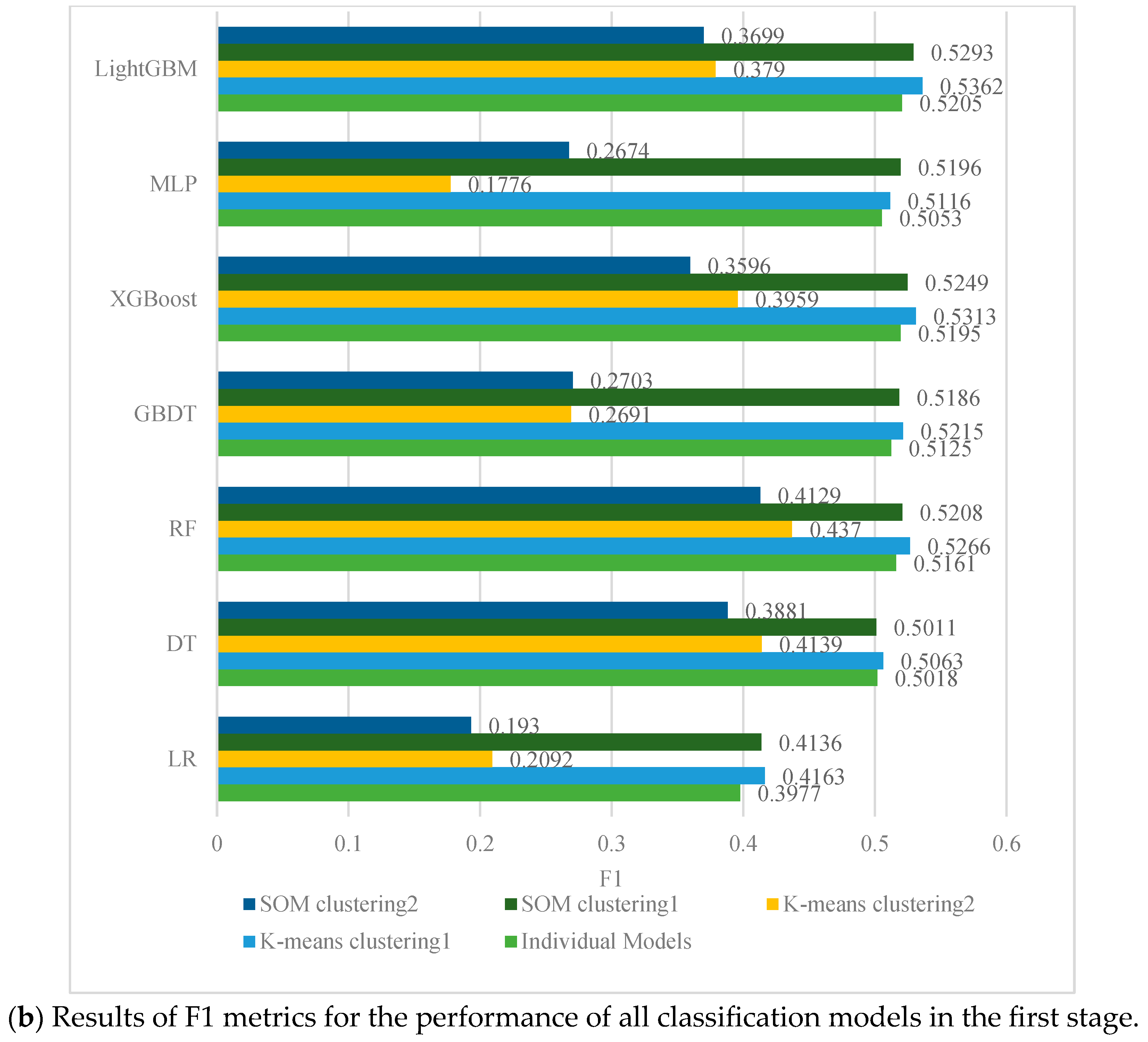
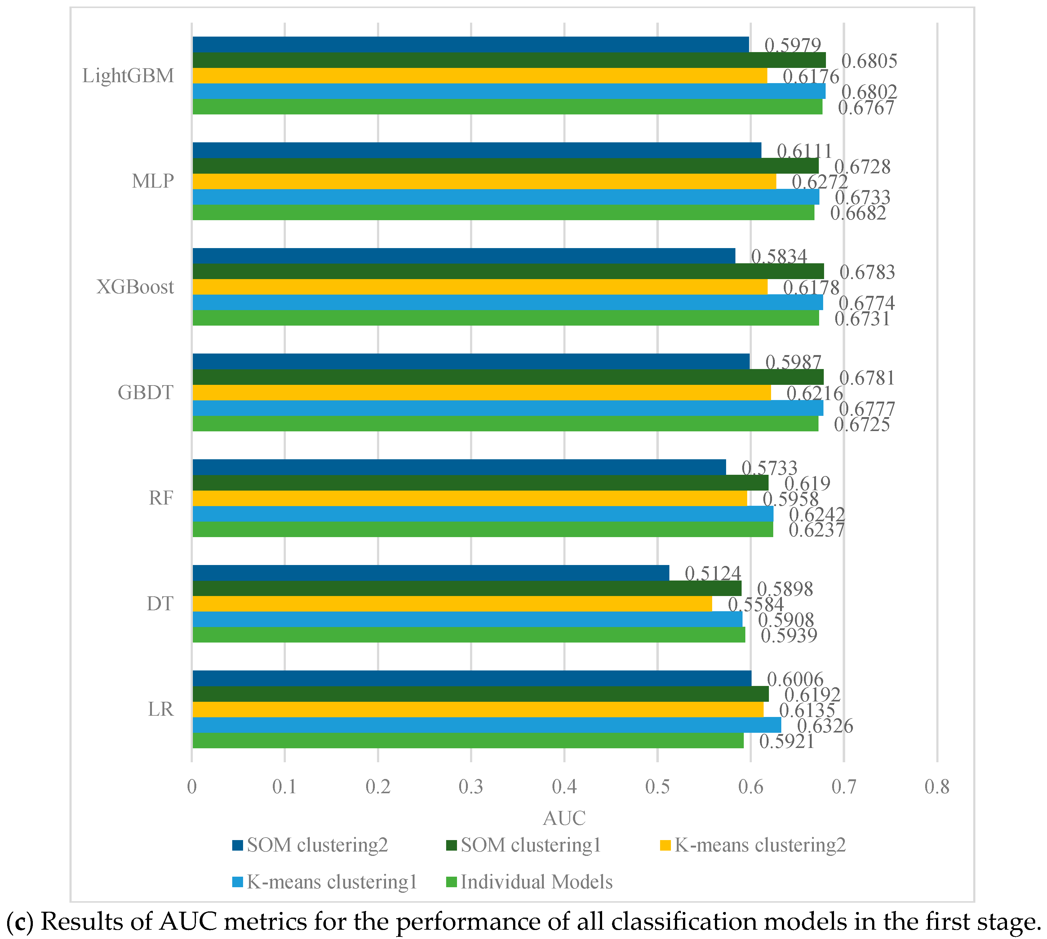
Figure 9 shows the results of the validation metrics for all the models in the first stage after adding two explanatory variables to the data features. The results show that the LightGBM, XGBoost, and GBDT models have a better predictive ability in predicting whether a firm incurs a loss, with AUC values of 0.6767, 0.6731, and 0.6725 in Figure 9c, and ACC values of 0.6348, 0.6313, and 0.6323 in Figure 9a, respectively. On the other hand, LR is the model with the worst prediction accuracy with an AUC value of 0.5921 and an ACC value of 0.6084. These results indicate that there is a slight improvement in ACC, F1, and AUC versus the individual models, without the addition of two explanatory variables in Table 4.

Furthermore, in the classification performance of the hybrid model predictions for the first stage after the addition of two explanatory variables in Figure 9, the results demonstrate that LightGBM and MLP have better predictive power and higher accuracy. The hybrid model predictions in Figure 9 have higher AUC, ACC and F1 values than the results without the addition of the two features in Table 4. For example, the AUC and ACC values of the best hybrid model in Table 4 are 0.6773 and 0.6341, respectively, while the AUC in Figure 9c and ACC values in Figure 9a of the best hybrid model are 0.6802 and 0.6375, respectively. On comparing the models, we find that adding two features results in significant improvements in AUC, ACC, F1, accuracy, and recall metrics. Thus, these results suggest that the addition of firm pertinent information and macroeconomic features improves the predictive performance of the first-stage classification (determining whether a firm incurs a loss).

In conclusion, the LightGBM model performs best during the first stage for the individual model classification metric in terms of predicting whether a firm incurs a loss, followed by the GBDT, XGBoost, and MLP models. In credit risk prediction, many complex non-linear factors exist, which can be better captured by these models, thus improving the performance. In terms of model selection and hyperparameter tuning, models such as LightGBM, GBDT, and XGBoost have mature tuning tools and techniques that can help optimise model performance. With the addition of pertinent small business information Real_Estate and economic recession features Recession to the model, the LightGBM model still has the best predictive power. LightGBM improves AUC and ACC by 0.73% and 0.79%, respectively, compared with the individual models, without the addition of the two variables. In the hybrid model classification metric for predicting whether a firm incurs a loss in the first stage, clustering makes the greatest improvement to the LR model, with the AUC value of LR rising from 0.5731 to 0.6161. The reason may be that clustering can reduce many feature dimensions into a few clusters. This alleviates the problem of dimensionality catastrophe in LR models and reduces the risk of model overfitting. In addition, clustering can divide data samples into clusters with similar features, which may help to reduce the problem of unbalanced categories. For linear models such as LR, a more balanced data distribution usually leads to better performance. It is evident from these results that the use of clustering methods on the US SBA credit dataset does help improve the performance of the models. With the addition of Real_Estate and Recession features, the hybrid model achieves higher values of AUC, ACC, and F1.

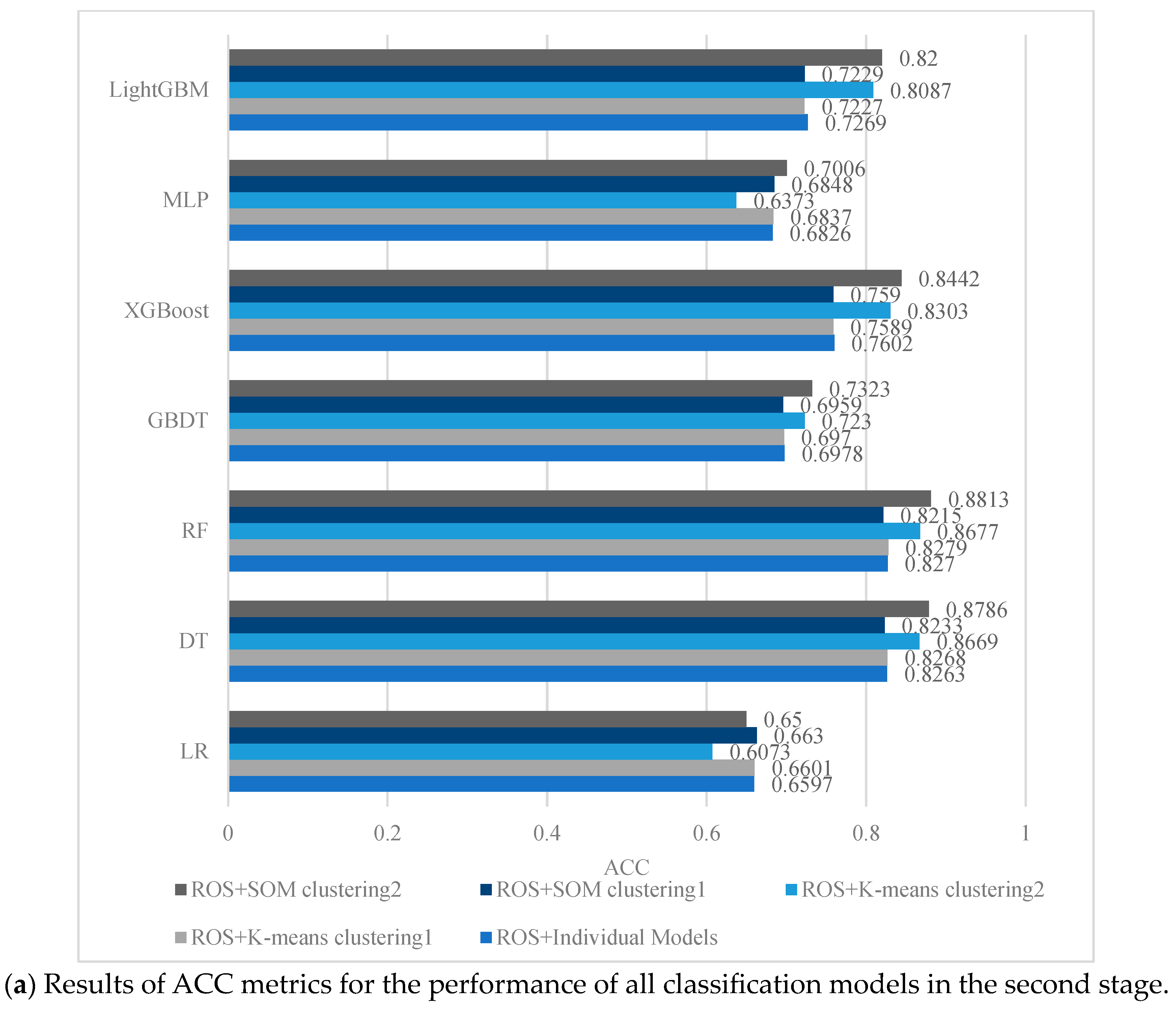
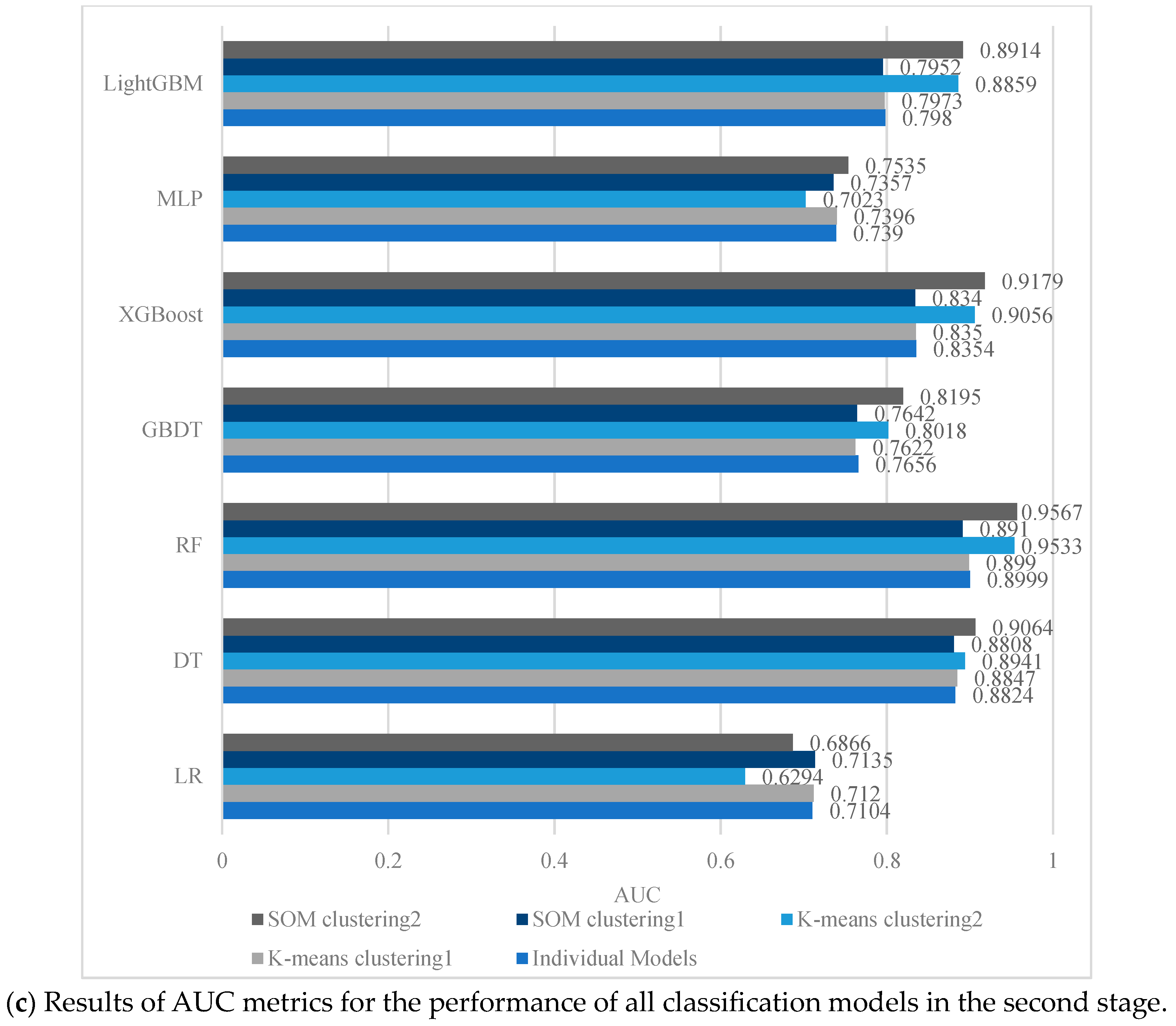
Figure 10 shows the classification validation metrics of the individual models and hybrid model for the second stage after the addition of two explanatory variables. For the prediction of whether a firm incurs a full loss by individual models, the results show that the benchmark LR model with the lowest predictive performance has an AUC value of 0.7104 in Figure 10c, which is almost close to the AUC (0.7105) of the LR model in Table 5. However, the RF model after ROS sampling has the best prediction with AUC, ACC, and F1 values of 0.8999, 0.827, and 0.8422, respectively. These results indicate substantial improvements in ACC, F1, and AUC versus the individual models in Table 5. This reflects the fact that the ROS (Random Oversampling) technique can help to improve the performance of the RF model by balancing the data distribution with the addition of a few more categories of samples, making it easier for the model to capture the occurrence of full-loss events.

For the classification prediction performance in the second stage of the hybrid model prediction process, these results show that considering different clusters, RF has the best prediction ability with the highest accuracy and the largest ACC (0.8813) in Figure 10a and AUC values (0.9567) in Figure 10c. Since different clusters may reflect different factors that influence full-loss events in specific domains, the RF model may better accommodate these domain-specific effects, improving the prediction performance under different clusters. The AUC, ACC and F1 results approach those without the addition of the two features in Table 5. Therefore, the hybrid model with the addition of two explanatory variables does not significantly improve the prediction performance in the second stage. This result echoes their weaker interpretability in conjunction with Figure 7, possibly because there is no strong correlation between these two explanatory variables for predicting whether a firm has a full-loss event.

So, in the second stage from the individual model classification metrics that predict whether a firm incurs a full loss, we find that RF has the best predictive performance after applying the ROS technique. With the addition of Real_Estate and Recession features, RF after applying ROS still has the best prediction performance with 0.73%, 0.45%, and 0.35% improvements in AUC, ACC, and F1, respectively. In the second stage of hybrid model classification prediction, the hybrid model after applying ROS is the best prediction model. However, the addition of the Real_Estate and Recession features has no significant enhancement in AUC, ACC, and F1. In conclusion, the hybrid model is beneficial for improving the accuracy of predicting whether a firm incurs a full loss in the second stage, but whether to add the two feature variables has little effect on the prediction results of the hybrid model.

To verify the LGD prediction performance of the HMS model for the third stage, we add the two explanatory features to the modelling, which follows the same process as shown in Section 4.4. The results are shown in

Table 7. Regression performance validation results for the LGD model.

	The Best Classification Model
Route	First stage	Second stage	Third stage	MSE	RMSE	MAE	$R^2$	EV
Route 1	LightGBM	ROS + RF	OLS	0.0993	0.3151	0.1858	0.4428	0.6015
Route 2	K-means (clustering 1 + LightGBM) and (clustering 2 + MLP)	ROS + RF		0.0983	0.3136	0.1848	0.4479	0.6042
	SOM (clustering 1 + LightGBM) and (clustering 2 + MLP)	ROS + RF		0.0992	0.3150	0.1859	0.443	0.6017
Route 3	Individual Models	ROS + K-means clustering + RF		0.0995	0.3155	0.186	0.4412	0.6006
	Individual Models	ROS + SOM clustering + RF		0.0992	0.315	0.1858	0.4429	0.6018
Route 4	K-means (clustering 1 + LightGBM) and (clustering 2 + MLP)	ROS + K-means clustering + RF		0.0986	0.314	0.1851	0.4464	0.6032
	K-means (clustering 1 + LightGBM) and (clustering 2 + MLP)	ROS + SOM clustering + RF		0.0983	0.3136	0.1848	0.4480	0.6045
	SOM (clustering 1 + LightGBM) and (clustering 2 + MLP)	ROS + K-means clustering + RF		0.0995	0.3154	0.1861	0.4414	0.6007
	SOM (clustering 1 + LightGBM) and (clustering 2 + MLP)	ROS + SOM clustering + RF		0.0992	0.315	0.1859	0.4430	0.602

.

Route 1 is the benchmark model for validation. First, comparing Route 1 and Route 2 in Table 7, we conclude that the hybrid model under Route 2 has a larger $R^2$ (0.4479) than Route 1’s $R^2$ (0.4428) and a slightly smaller MAE (0.1848) than that of Route 1 (0.1858). Second, comparing Route 1 and Route 3, we observe that $R^2$ (0.4429) and EV (0.6018) of the hybrid model for Route 3 are larger than the $R^2$ (0.4428) and EV (0.6015) of the benchmark Route 1. Third, comparing the optimal $R^2$ of the hybrid model under Route 3, we find a 1.15% improvement in the $R^2$ (0.448) of the hybrid model for Route 4. Route 4 has the largest $R^2$ and EV (0.6045), whose MSE (0.0983), RMSE (0.3136), and MAE (0.1848) are also the smallest among those under all the routes. Therefore, this validates that the HMS model under Route 4 is the optimal model prediction model for multi-stage LGD prediction. The clustering step is introduced one by one for each additional route, with Route 4 achieving the highest predictive performance, suggesting that the hybrid model is better able to capture the complexity of the data or that there are complementarities between the individual models, then it may exhibit higher $R^2$.

In a word, for all the multi-stage LGD prediction models, we analyse the MSE, RMSE and MAE metrics under the four routes in Figure 2. The hybrid model under Route 2 in Table 6 has a slightly higher $R^2$ of 0.06% and a slightly lower MAE of 0.05% than those under Route 1. The hybrid model under Route 3 improves the $R^2$ and EV by 0.22% and 0.15%, respectively, versus the $R^2$ and EV of the benchmark Route 1. The $R^2$ of the hybrid model under Route 4 improves by 0.3% over the $R^2$ of the benchmark Route 1. This route has the largest $R^2$ and EV, and the smallest MSE, RMSE, and MAE, so is the optimal model prediction route for multi-stage LGD prediction. The ROS strategy helps to address the sample imbalance problem, especially in credit risk analysis, which can improve the prediction performance for full-loss events. The combination of these strategies makes Route 4 the best model prediction path. Thus, the HMS model of Route 4 takes full advantage of unsupervised clustering and ROS to improve the performance of multi-stage LGD prediction with minimum $R^2$ and maximum EV values. This is important for credit risk analysis and decision making. With the addition of the Real_Estate and Recession features, the results still show that the best prediction performance is achieved under Route 4, which consists of the HMS model, whose $R^2$ increases by 1.17% over that under Route 1. Thus, the HMS model is effective in improving the accuracy of multi-stage LGD prediction.

4.6. Discussion

Following the results in Section 4.2, Section 4.3, Section 4.4 and Section 4.5, we several observations and comparisons. We analyse the predictive performance of the model for three stages, specifically predicting whether the firm suffers losses in the first stage, predicting whether the firm suffers a full loss in the second stage, and predicting the overall LGD of the commercial bank, and compare the HMS model with other models. In addition, we analyse the inclusion of the variables Real_Estate and Recession in our models, as summarised below.

First, the HMS model is better than models currently in use, e.g., the LossCale model of Moody’s LGD prediction [53]. This is because Moody’s regression model may have small predictive performance in some cases. The HMS model uses a multi-stage modelling approach to predict credit losses at different stages separately. This approach can better capture the complexity and diversity of credit losses as different stages may involve different risk factors and prediction models. Moody’s regression modelling may prefer to integrate all information into one model and may ignore the differences between stages.

Second, the addition of the two features significantly improves the predictive accuracy of the classification model. The HMS model performs consistently well overall. This suggests that the two features should be considered to improve the accuracy of commercial banks’ LGD prediction.

Finally, the use of the SHAP interpretability methodology for the HMS model can help to explain the model’s predictions by providing insights about the impact of each feature on the prediction of each stage. Different features in different stages of credit risk prediction have different importance for different types of credit losses (whether a loss occurs, full loss, partial loss). Within each stage, financial indicators such as DisbursementGross and Real_estate have a high level of importance, reflecting their key role in credit risk assessment. Portion and economic environment factors (e.g., Recession) also have an impact on the prediction of credit losses, while their importance may vary from stage to stage. These insights can help banks better understand risk factors, develop more accurate credit policies, and help companies improve their financial and operational strategies to reduce credit risk. It also highlights the importance of considering different features at different stages of the process to assess credit risk more accurately.

In summary, the HMS model is more effective for multi-stage LGD prediction, which helps reach an optimal route. In a practical sense, in terms of risk assessment and decision making, understanding which features have the greatest impact on the risk of loss can help financial institutions better assess and manage risk. They can pay more attention to key characteristics such as Real_Estate and Portion, economic recession, etc., to formulate more rational credit policies. For businesses, understanding what factors may affect their risk of loss can help them improve their financial and operational strategies to reduce risk and increase financial stability. Therefore, assessing the significance of features can help financial institutions and businesses better understand risk factors and thus develop more accurate decisions and strategies.

5. Conclusions

In this study, we propose a new HMS model for predicting multi-stage LGD and test it on both an original dataset and a validation set. We then compare the overall LGD prediction performance of the models under four routes from the perspective of different evaluation metrics. In addition, we add pertinent firm information and macroeconomic features for robustness checking of the results. We find that the HMS model outperforms the models under other routes in predicting multi-stage LGD. While the literature ignores latent firm information, we find that the classification prediction performance of the HMS model is higher when considering such features. Our results confirm the superiority of the new approach and increase our confidence that it can be generalised to make predictions based on other credit datasets of financial institutions, especially Peer-to-Peer (P2P) firms in China. In the financial field, P2P usually refers to individuals or firms borrowing or lending money directly to other individuals or firms through an online platform, bypassing traditional financial institutions such as banks. This hopefully will facilitate future theoretical and empirical research on combining unsupervised learning techniques with supervised learning models and help develop more effective combinatorial strategies. In addition, the HMS model uses the SHAP method to provide an interpretable explanation of the impact of each feature on the predictions. This helps to understand the model’s predictions and identify the most important risk factors.

In practice, financial institutions can use the HMS model for credit risk assessment to assess the credit risk of borrowers and formulate appropriate credit policies more accurately. Next, financial institutions may use the HMS model to calculate the required credit loss capital to assure that regulatory requirements are met. Future research could make modifications or additions to our work in several areas. First, in terms of dealing with outliers, we remove outliers to build better-fitting models or to produce statistically significant results. However, outliers arise from the natural variability of LGD predictions, and our removal of these outliers may improve the fit statistics but not the predictive power of the model. In the future, we can use robust regression to reduce the impact of outliers in our models and comparative analyses can be performed with and without outliers to show the difference in results. In addition, if possible, incorporating more recent data sources into the model may improve its performance. This includes new financial data, macroeconomic data, industry data, and so on. Second, the forecasting of LGD is usually influenced by time factors. Different market conditions, economic environments, and financial situations may exist at different points in time, and these factors can influence the extent of credit losses. In the future, we can further investigate the impact of the business cycle on LGD. Finally, more pertinent firm information and possible interaction effects could be explored to improve the predictive probability of LGD.

References

1. Louzada, F.; Ara, A.; Fernandes, G.B. Classification methods applied to credit scoring: Systematic review and overall comparison. Surv. Oper. Res. Manag. Sci. 2016, 21, 117–134. [Google Scholar] [CrossRef]
2. Machado, M.R.; Karray, S. Assessing credit risk of commercial customers using hybrid machine learning algorithms. Expert Syst. Appl. 2022, 200, 116889. [Google Scholar] [CrossRef]
3. Twala, B. Combining classifiers for credit risk prediction. J. Syst. Sci. Syst. Eng. 2009, 18, 292–311. [Google Scholar] [CrossRef]
4. Basel Committee on Banking Supervision. Overview of The New Basel Capital Accord; Bank for International Settlements: Basel, Switzerland, 2003. [Google Scholar]
5. Gürtler, M.; Hibbeln, M. Improvements in loss given default forecasts for bank loans. J. Bank. Financ. 2013, 37, 2354–2366. [Google Scholar] [CrossRef]
6. Bellotti, T.; Crook, J. Loss given default models incorporating macroeconomic variables for credit cards. Int. J. Forecast. 2012, 28, 171–182. [Google Scholar] [CrossRef]
7. Calabrese, R.; Zanin, L. Modelling spatial dependence for Loss Given Default in peer-to-peer lending. Expert Syst. Appl. 2022, 192, 116295. [Google Scholar] [CrossRef]
8. Serrano-Cinca, C.; Gutiérrez-Nieto, B. The use of profit scoring as an alternative to credit scoring systems in peer-to-peer (P2P) lending. Decis. Support Syst. 2016, 89, 113–122. [Google Scholar] [CrossRef]
9. Zhang, J.; Thomas, L.C. Comparisons of linear regression and survival analysis using single and mixture distributions approaches in modelling LGD. Int. J. Forecast. 2012, 28, 204–215. [Google Scholar] [CrossRef]
10. Kellner, R.; Nagl, M.; Rösch, D. Opening the black box–Quantile neural networks for loss given default prediction. J. Bank. Financ. 2022, 134, 106334. [Google Scholar] [CrossRef]
11. Loterman, G.; Brown, I.; Martens, D.; Mues, C.; Baesens, B. Benchmarking regression algorithms for loss given default modeling. Int. J. Forecast. 2012, 28, 161–170. [Google Scholar] [CrossRef]
12. Li, K.; Zhou, F.; Li, Z.; Yao, X.; Zhang, Y. Predicting loss given default using post-default information. Knowl.-Based Syst. 2021, 224, 107068. [Google Scholar] [CrossRef]
13. Lucas, A. Basel II Problem Solving, QFRMC Workshop and Conference on Basel II & Credit Risk Modelling in Consumer Lending; University of Southampton: Southampton, UK, 2006. [Google Scholar]
14. Tanoue, Y.; Kawada, A.; Yamashita, S. Forecasting loss given default of bank loans with multi-stage model. Int. J. Forecast. 2017, 33, 513–522. [Google Scholar] [CrossRef]
15. Bao, W.; Lianju, N.; Yue, K. Integration of unsupervised and supervised machine learning algorithms for credit risk assessment. Expert Syst. Appl. 2019, 128, 301–315. [Google Scholar] [CrossRef]
16. Li, M.; Mickel, A.; Taylor, S. “Should This Loan be Approved or Denied?”: A Large Dataset with Class Assignment Guidelines. J. Stat. Educ. 2018, 26, 55–66. [Google Scholar] [CrossRef]
17. Shi, B.; Chi, G.; Li, W. Exploring the mismatch between credit ratings and loss-given-default: A credit risk approach. Econ. Model. 2020, 85, 420–428. [Google Scholar] [CrossRef]
18. Shi, B.; Zhao, X.; Wu, B.; Dong, Y. Credit rating and microfinance lending decisions based on loss given default (LGD). Financ. Res. Lett. 2019, 30, 124–129. [Google Scholar] [CrossRef]
19. Xing, H.; Sun, N.; Chen, Y. Credit rating dynamics in the presence of unknown structural breaks. J. Bank. Financ. 2012, 36, 78–89. [Google Scholar] [CrossRef]
20. Bijak, K.; Thomas, L.C. Does segmentation always improve model performance in credit scoring? Expert Syst. Appl. 2012, 39, 2433–2442. [Google Scholar] [CrossRef]
21. Jankowitsch, R.; Pullirsch, R.; Veža, T. The delivery option in credit default swaps. J. Bank. Financ. 2008, 32, 1269–1285. [Google Scholar] [CrossRef]
22. Calabrese, R.; Zenga, M. Bank loan recovery rates: Measuring and nonparametric density estimation. J. Bank. Financ. 2010, 34, 903–911. [Google Scholar] [CrossRef]
23. Renault, O.; Scaillet, O. On the way to recovery: A nonparametric bias free estimation of recovery rate densities. J. Bank. Financ. 2004, 28, 2915–2931. [Google Scholar] [CrossRef]
24. Acharya, V.V.; Bharath, S.T.; Srinivasan, A. Does industry-wide distress affect defaulted firms? Evidence from creditor recoveries. J. Financ. Econ. 2007, 85, 787–821. [Google Scholar] [CrossRef]
25. Altman, E.I.; Brady, B.; Resti, A.; Sironi, A. The link between default and recovery rates: Theory, empirical evidence, and implications. J. Bus. 2005, 78, 2203–2228. [Google Scholar] [CrossRef]
26. Bade, B.; Rösch, D.; Scheule, H. Default and recovery risk dependencies in a simple credit risk model. Eur. Financ. Manag. 2011, 17, 120–144. [Google Scholar] [CrossRef]
27. Papke, L.E.; Wooldridge, J.M. Econometric methods for fractional response variables with an application to 401 (k) plan participation rates. J. Appl. Econom. 1996, 11, 619–632. [Google Scholar] [CrossRef]
28. Barboza, F.; Kimura, H.; Altman, E. Machine learning models and bankruptcy prediction. Expert Syst. Appl. 2017, 83, 405–417. [Google Scholar] [CrossRef]
29. Bastos, J.A. Forecasting bank loans loss-given-default. J. Bank. Financ. 2010, 34, 2510–2517. [Google Scholar] [CrossRef]
30. Moscatelli, M.; Parlapiano, F.; Narizzano, S.; Viggiano, G. Corporate default forecasting with machine learning. Expert Syst. Appl. 2020, 161, 113567. [Google Scholar] [CrossRef]
31. Yao, X.; Crook, J.; Andreeva, G. Support vector regression for loss given default modelling. Eur. J. Oper. Res. 2015, 240, 528–538. [Google Scholar] [CrossRef]
32. Bellotti, A.; Brigo, D.; Gambetti, P.; Vrins, F. Forecasting recovery rates on non-performing loans with machine learning. Int. J. Forecast. 2021, 37, 428–444. [Google Scholar] [CrossRef]
33. Hurlin, C.; Leymarie, J.; Patin, A. Loss functions for loss given default model comparison. Eur. J. Oper. Res. 2018, 268, 348–360. [Google Scholar] [CrossRef]
34. Kaposty, F.; Kriebel, J.; Löderbusch, M. Predicting loss given default in leasing: A closer look at models and variable selection. Int. J. Forecast. 2020, 36, 248–266. [Google Scholar] [CrossRef]
35. Miller, P.; Töws, E. Loss given default adjusted workout processes for leases. J. Bank. Financ. 2018, 91, 189–201. [Google Scholar] [CrossRef]
36. Gholamian, M.; Jahanpour, S.; Sadatrasoul, S. A new method for clustering in credit scoring problems. J. Math. Comput. Sci. 2013, 6, 97–106. [Google Scholar] [CrossRef]
37. Luo, S.-T.; Cheng, B.-W.; Hsieh, C.-H. Prediction model building with clustering-launched classification and support vector machines in credit scoring. Expert Syst. Appl. 2009, 36, 7562–7566. [Google Scholar] [CrossRef]
38. Yu, L.; Yue, W.; Wang, S.; Lai, K.K. Support vector machine based multiagent ensemble learning for credit risk evaluation. Expert Syst. Appl. 2010, 37, 1351–1360. [Google Scholar] [CrossRef]
39. Zhang, F.; Tadikamalla, P.R.; Shang, J. Corporate credit-risk evaluation system: Integrating explicit and implicit financial performances. Int. J. Prod. Econ. 2016, 177, 77–100. [Google Scholar] [CrossRef]
40. AghaeiRad, A.; Chen, N.; Ribeiro, B. Improve credit scoring using transfer of learned knowledge from self-organizing map. Neural Comput. Appl. 2017, 28, 1329–1342. [Google Scholar] [CrossRef]
41. Huysmans, J.; Baesens, B.; Vanthienen, J.; Van Gestel, T. Failure prediction with self organizing maps. Expert Syst. Appl. 2006, 30, 479–487. [Google Scholar] [CrossRef]
42. Papouskova, M.; Hajek, P. Two-stage consumer credit risk modelling using heterogeneous ensemble learning. Decis. Support Syst. 2019, 118, 33–45. [Google Scholar] [CrossRef]
43. Caruso, G.; Gattone, S.; Fortuna, F.; Di Battista, T. Cluster Analysis for mixed data: An application to credit risk evaluation. Socio-Econ. Plan. Sci. 2021, 73, 100850. [Google Scholar] [CrossRef]
44. Kohonen, T. The self-organizing map. Proc. IEEE 1990, 78, 1464–1480. [Google Scholar] [CrossRef]
45. Coenen, L.; Verbeke, W.; Guns, T. Machine learning methods for short-term probability of default: A comparison of classification, regression and ranking methods. J. Oper. Res. Soc. 2022, 73, 191–206. [Google Scholar] [CrossRef]
46. Qi, M.; Zhao, X. Comparison of modeling methods for loss given default. J. Bank. Financ. 2011, 35, 2842–2855. [Google Scholar] [CrossRef]
47. Munkhdalai, L.; Munkhdalai, T.; Namsrai, O.-E.; Lee, J.Y.; Ryu, K.H. An empirical comparison of machine-learning methods on bank client credit assessments. Sustainability 2019, 11, 699. [Google Scholar] [CrossRef]
48. Xia, Y.; Zhao, J.; He, L.; Li, Y.; Yang, X. Forecasting loss given default for peer-to-peer loans via heterogeneous stacking ensemble approach. Int. J. Forecast. 2021, 37, 1590–1613. [Google Scholar] [CrossRef]
49. Olson, L.M.; Qi, M.; Zhang, X.; Zhao, X. Machine learning loss given default for corporate debt. J. Empir. Financ. 2021, 64, 144–159. [Google Scholar] [CrossRef]
50. de Lange, P.E.; Melsom, B.; Vennerød, C.B.; Westgaard, S. Explainable AI for Credit Assessment in Banks. J. Risk Financ. Manag. 2022, 15, 556. [Google Scholar] [CrossRef]
51. Moscato, V.; Picariello, A.; Sperlí, G. A benchmark of machine learning approaches for credit score prediction. Expert Syst. Appl. 2021, 165, 113986. [Google Scholar] [CrossRef]
52. Brito, L.C.; Susto, G.A.; Brito, J.N.; Duarte, M.A. An explainable artificial intelligence approach for unsupervised fault detection and diagnosis in rotating machinery. Mech. Syst. Signal Process. 2022, 163, 108105. [Google Scholar] [CrossRef]
53. Gupton, G.M.; Stein, R.M.; Salaam, A.; Bren, D. LossCalcTM: Model for Predicting Loss Given Default (LGD); Moody’s KMV: New York, NY, USA, 2002. [Google Scholar]
Figure 1. Diagram of the main idea of the HMS model.
Systems 11 00505 g001
Figure 2. Diagrams of different integrated methods under four routes.
Systems 11 00505 g002
Figure 3. Experimental process for the HMS model.
Systems 11 00505 g003
Figure 4. Distribution and boundary points of LGDs. Note: The two dashed represent the partition lines for x = 0.05 and x = 0.97, respectively.
Systems 11 00505 g004
Figure 5. Cluster mapping describing data states.
Systems 11 00505 g005aSystems 11 00505 g005b
Figure 6. SHAP feature importance ranking of variables for the first stage.
Systems 11 00505 g006
Figure 7. SHAP feature importance ranking of variables for the second stage.
Systems 11 00505 g007
Figure 8. Ranking of OLS absolute coefficients of variables in the third stage.
Systems 11 00505 g008
Figure 9. Classification performance validation results for the first stage.
Systems 11 00505 g009aSystems 11 00505 g009bSystems 11 00505 g009c
Figure 10. Classification performance validation results for the second stage.
Systems 11 00505 g010aSystems 11 00505 g010bSystems 11 00505 g010c