Motor Vehicle Insurance Anti-Fraud Modeling Based on a Stochastic Differential Game System

Abstract

In this paper, we regard policyholders, insurance companies, and government departments to be an anti-fraud supervision system, and we explore the supervision of motor vehicle insurance fraud from the perspective of a tripartite game. Taking into consideration the bad reputation records of policyholders as a state variable, through continuous accumulation in effective time, it creates a continuous growth-type warning effect on policyholders, and thus, effectively curbs policyholder fraud and false supervision by insurance companies. At the same time, by considering the influence of random factors on the anti-fraud game of motor vehicle insurance, in this paper, we establish a stochastic differential game model to explore the optimal strategy, the optimal income level, and the expectation and variance of the insured’s bad reputation record stock under the conditions of with and without government supervision. Finally, through a simulation analysis, it is found that the game with government supervision is more conducive to reduce the insured’s fraud intensity, and the simulation proves the impact of different parameters on system stability.

1. Introduction

Motor vehicle insurance has always been an important field in China’s insurance market. According to the annual operating data of the insurance industry released by China’s Insurance Regulatory Commission, the national auto insurance premium income, in 2021, reached 777.3 billion yuan, accounting for 56.8% of property insurance premiums. Nevertheless, auto insurance is the basic business of property insurance companies; however, the phenomenon of insurance fraud is also increasing. According to the “2019 China’s Insurance Industry Intelligent Risk Control White Paper”, auto insurance fraud in China is the hardest hit area of insurance fraud. Auto insurance fraud accounts for as much as 80% of insurance fraud, with conservative estimates suggesting that the amount involved is as high as 20 billion yuan per year. According to the daily economic news report, the proportion of malicious surrender, hedging, and fraud is 5% in traditional insurance companies, while the proportion in Internet insurance companies and Internet platforms is as high as 30% to 40%. As of 6 January 2021, there were 4839 articles on the theme of ”insurance fraud” in the Web of Science database, while there were less than 50 articles on the theme of ”auto insurance fraud” in the Web of Science database [1]. This shows that there is still insufficient research on auto insurance fraud.

Insurance fraud is a major challenge facing the insurance industry. Its existence seriously hinders the normal operation of insurance companies, disrupts the order of the insurance market, and thus, infringes on the economic interests of honest insured farmers. Therefore, there is a need to analyze insurance fraud. In recent years, research efforts on insurance fraud at home and abroad have mainly focused on analyses of the causes of fraud to assist in developing regulatory recommendations, the use of machine learning technology to identify customers’ fraudulent claims, and the establishment of fraud evolutionary game analysis. In terms of game models, Zheng Jun (2020) analyzed a tripartite game model of ”farmers, insurance companies, and government”, and believed that the government should innovate the current subsidy model, refine the previous subsidy subjects, and take into account the benefits of insurance companies in the process of subsidy [2]. Qiao Xin (2021) established a tripartite game among the insured, the insurance company, and the government, and added a reputation loss mechanism to study agricultural insurance fraud problems [3]. In terms of analyzing the causes of fraud, De Warren (2016) studied the unethical behavior of policyholders, integrated the impact of moral hazard on the insurance industry, and pointed out that the root cause of insurance fraud was moral hazard, especially the moral hazard of policyholders, which would ultimately affect the effective operation of the insurance industry [4]. Ishida et al. (2016) studied insurance fraud from three aspects: moral strength, moral consciousness, and moral judgment, based on independent samples of two age stages [5]. There are also relevant studies in the literature on the impact of insurance fraud factors on fraud from an empirical perspective. In fraud identification, Tang, Z. Q. (2022) proposed using deep learning technology to detect wheat lodging and to prevent farmers from exaggerating losses [6]. Yan (2019) used an improved genetic algorithm and optimized the BP neural network to identify auto insurance fraud [7]. Xia (2022) combined convolutional neural networks (CNNs), long short-term memory (LSTM), and deep neural networks (DNNs) and proposed a deep learning model for auto insurance fraud identification [8]. In view of the fact that motor vehicle insurance anti-fraud detection technology continues to be based on traditional machine learning, relevant studies in the literature have discussed motor vehicle insurance anti-fraud detection technology under the background of big data, and have proposed the use of related outlier detection, collusion relationship detection, and other technologies for fraud detection [9].

In order to reduce the occurrence of motor vehicle insurance fraud, we need to accomplish effective identification and detection of potential fraudulent policyholders, and we also need to take corresponding measures to effectively curb the fraudulent behavior of policyholders. The process of providing motor vehicle insurance involves a certain contradiction between the mutual interests of each subject. Each subject, as much as possible, tries to grasp more favorable information to constantly improve its own strategy according to the strategies of other parties, thus, forming a dynamic cycle, which promotes the continuous evolution and development of the motor vehicle insurance market. For insurance activities and games, the interaction between two participants is the most basic activity, and can show the basic characteristics of the activity. Therefore, it is feasible to use game theory to study insurance fraud [10]. In recent years, many scholars have proposed corresponding regulatory strategies and punishment strategies from the perspective of game theory. For example, He (2022) established an evolutionary game model that consisted of two players, i.e., the insured and the insurance company, and used the replicator dynamics equation to analyze the equilibrium point and stability of the strategies of both parties, thus, further proposing corresponding policy recommendations [11]. Rubinstein and Yaari (1983) proved that, in an infinitely repeated game model, the insurer connected the behavior of the insured with the level of the rate charged, which made the insured care about the insurance cost, thus, eliminating the moral hazard problem [12]. Wu (2022) established a tripartite evolutionary game. By finding the equilibrium point of the game system and discussing the strategic choices of participants under different model parameters, he enriched the existing research on financial fraud and audit supervision [13]. Dong (2022) proposed an evolutionary game analysis from the perspective of dynamic incentive and punishment. The results showed that it was easier to maintain stability in a system of dynamic incentive and punishment than in a system of static incentive and punishment [14]. Ma Cui (2017) used game-related theory as an analytical tool to establish a game matrix between regulators and insurance operators, and thereby, established a Nash equilibrium of mixed strategies and analyzed the necessity of insurance regulation [15]. Based on the above game theory, we have found that most of the above-mentioned game approaches in the literature have not considered the social point of view, and have often ignored the reputation loss of the parties, insurance companies, and government departments after the occurrence of fraudulent incidents. However, in real life, reputation loss caused by fraudulent incidents is often huge. In the literature, although Qiao Xin (2021) established a tripartite game among the insured, the insurance company, and the government, and added a reputation loss mechanism to study the problem of motor vehicle insurance fraud, only a simulation was used to obtain the tripartite evolution state when the system was stable, and the conditions for the tripartite game system to reach a stable state were not analyzed, which was not conducive to readers and relevant departments to propose effective anti-fraud policies.

At present, no scholar has applied a differential game to the supervision of motor vehicle insurance fraud. In fact, differential games are important dynamic games, and differential games are used in many fields [16]. For example, more abundant research results have been achieved in supply chain low-carbon emission reduction [17,18], the power market [19], quality problem control [20,21], environmental governance [22,23,24], and other fields. Considering the excellent effects of differential games in various fields, in this paper, we innovatively apply a differential game to motor vehicle insurance anti-fraud, and consider the interference of random factors such as climate, environment, and policy on motor vehicle insurance fraud. Therefore, in this paper, we refer to the existing literature on handling random interference [25,26,27] to construct a stochastic differential game model. We consider that the fraudulent behavior of the insured will produce a bad reputation record, and the insured’s reputation problem, as one of the core issues of a reward and punishment system, can provide the insured with constant vigilance. A bad reputation record is a stock that accumulates over a period of validity, and does not immediately disappear after a game. It increases or decreases over time. Bad reputation accumulation limits the various behaviors of the insured, and also affects the premium pricing of the insured, thus, affecting the interests of all parties involved in the operation of insurance. In this paper, we consider the reputation mechanism and conduct anti-fraud modeling of motor vehicle insurance based on a tripartite stochastic differential game. Firstly, we discuss the equilibrium solution of policyholders and insurance companies without government regulation. Then, we discuss the equilibrium solution of all parties with government regulation. Finally, we compare the two models through a simulation, and show the influence of important parameters on the equilibrium solution of the model.

The main work of this paper is as follows: In Section 1, we introduce the background of motor vehicle insurance and the harm associated with insurance fraud, and we introduce several methods of anti-insurance fraud; in Section 2, we establish a stochastic differential game system without government supervision, and obtain the optimal strategy of the system participants, the optimal income level, and the expectation and variance of the insured’s bad reputation record stock under the condition of no government supervision; in Section 3, we establish a stochastic differential game system under government supervision, and obtain the optimal strategy of the system participants, the optimal income level, and the expectation and variance of the insured’s bad reputation record stock under the condition of government supervision; in Section 4, we conduct a simulation test to verify the influence of each parameter on the participant strategy; in Section 5, we provide a summary.

The innovation points of this article are: (1) This article is not limited to a game between the insured and the insurance company, but we also include the government regulatory department to realize the government’s role in supervising the insurance company and the insured. (2) We introduce a differential game into motor vehicle insurance anti-fraud. (3) We consider random interference in motor vehicle insurance fraud, and we introduce random interference into the anti-fraud differential game of motor vehicle insurance.

2. Stochastic Differential Game Model without Government Regulation

Hypothesis 1: 

Taking the bad reputation record stock of the insured as the state variable, the supervision of the insurance company, and the fraud of the insured as the control variables, and considering the natural attenuation of the bad reputation record, the change process of the bad reputation record of the insured over time is [27]:

$$M(t)={\epsilon }_1{g}_1(t)u(t)-\delta M(t)$$

(1)

Among them, $M(t)$ is the cumulative amount of bad reputation of the insured at time $t$. ${\epsilon }_1\in [0,1]$ is the regulatory success rate of insurance companies. $g_1(t)>0$ is the strength of supervision of the insurance company at time $t$. $u(t)>0$ is the fraud intensity of the insured at time $t$. $\delta >0$ is the decay rate of policyholders’ bad reputation accumulation, which is usually caused by the lack of supervision of insurance companies and government departments.

In the problem of motor vehicle insurance fraud, the influence of random factors such as climate, environment, and policy will interfere with the bad reputation record. Therefore, considering the random disturbance problem faced by the system, in this paper, we construct the process of bad reputation record changing with time under random disturbance:

$$dM(t)=[{\epsilon }_1{g}_1(t)u(t)-\delta M(t)]dt+\sigma [M(t)]d\omega (t)$$

(2)

Hypothesis 2: 

In this paper, we assume that the change rule of bad reputation record stock with time is affected by the Wiener process, $\sigma [M(t)]$ is the random disturbance influence coefficient, $\omega (t)$ is the standard Wiener process, and we assume that the random disturbance influence coefficient is proportional to the square root of the bad reputation record stock [28], that is, $\sigma [M(t)]d\omega (t)=\sigma \sqrt{M}d\omega (t)$.

Hypothesis 3: 

In motor vehicle insurance fraud management, the fraud consumption cost of policyholders has a certain correlation with fraud intensity. Usually, with an increase in fraud intensity, the fraud cost is also generally increased. Therefore, considering the convexity of the cost, in this paper, we use a convex function to describe the relationship between the fraud intensity of the policyholder and the fraud cost, so that the fraud cost of the policyholder is $\frac{b_1}{2}u{(t)}^2$, where $b_1$ is the fraud cost coefficient of the insured. Similarly, the regulatory cost of insurance companies has a similar correlation with their regulatory intensity, therefore, it is assumed to be the regulatory cost $\frac{b_2}{2}{g}_1{(t)}^2$ of insurance companies, where $b_2$ is the regulatory cost coefficient of insurance companies.

Hypothesis 4: 

During the insured period of insurance, the participants have the same discount rate $\rho$ at any time, and $\rho >0$.

Based on the above assumptions, and considering that the insured and an insurance company are both rational subjects, that is, the purpose of the participants is to seek the fraud management strategy under their own maximum interests, according to the general hypothesis, the income function obtained by the participants through their own efforts is linearly related to the degree of effort of the parties, and the income function of the following participants is obtained by referring to the setting method of the objective function in the differential game:

Income function of the insured:

$${\displaystyle {\int }_0^t{e}^{-\rho t}}[Q_1+\alpha u(t)-\frac{b_1}{2}u{(t)}^2-fM(t)]dt$$

(3)

Income function of the insurance company:

$${\displaystyle {\int }_0^t{e}^{-\rho t}}[Q_2-\alpha u(t)-\frac{b_2}{2}{g}_1{(t)}^2+fM(t)]dt$$

(4)

The income of the policyholders’ fraud is set as a linear function of the fraud intensity. Let $\alpha u(t)$ be the claim income of the policyholders’ fraud; $\alpha >0$ is the coefficient of the policyholders’ fraud income; $Q_1$ and $Q_2$ are the basic income of the policyholder and the insurance company, respectively; $f$ represents the insurance company’s punishment (increase premiums, reduce priority services, etc.) coefficient for bad reputation policyholders.

Theorem 1. 

In the absence of government supervision, the optimal fraud probability of the insured is:

$$u^{\ast }=\frac{a{b}_2{(\delta +\rho )}^2}{b_1{b}_2{(\delta +\rho )}^2+f^2{\epsilon }_1^2}$$

(5)

In the absence of government supervision, the optimal effort of the insurance company is:

$$g_1^{\ast }=\frac{f{\epsilon }_{1}a(\rho +\delta )}{b_1{b}_2{(\rho +\delta )}^2+f^2{\epsilon }_1^2}$$

(6)

The proof is shown in Appendix A.

Theorem 2. 

Without government regulation, the optimal benefits of policyholders are:

$$\begin{array}{l}{V}_u=\frac{-f}{\rho +\delta }M+\frac{1}{\rho }\{Q_1+\frac{a{b}_2{(\delta +\rho )}^2}{b_1{b}_2{(\delta +\rho )}^2+f^2{\epsilon }_1^2}\\ (\alpha -\frac{b_1}{2}\frac{a{b}_2{(\delta +\rho )}^2}{b_1{b}_2{(\delta +\rho )}^2+f^2{\epsilon }_1^2}+\\ \frac{-f}{\rho +\delta }{\epsilon }_1\frac{f{\epsilon }_{1}a(\rho +\delta )}{b_1{b}_2{(\rho +\delta )}^2+f^2{\epsilon }_1^2})\}\end{array}$$

(7)

Without government regulation, the optimal benefits of the insurance company are:

$$\begin{array}{l}{V}_{g_1}=\frac{f}{\rho +\delta }M+\frac{1}{\rho }\{Q_2-\frac{{\alpha }^2{b}_2{(\delta +\rho )}^2}{b_1{b}_2{(\delta +\rho )}^2+f^2{\epsilon }_1^2}\\ +\frac{f{\epsilon }_{1}a(\rho +\delta )}{b_1{b}_2{(\rho +\delta )}^2+f^2{\epsilon }_1^2}[-\frac{b_2}{2}\frac{f{\epsilon }_{1}a(\rho +\delta )}{b_1{b}_2{(\rho +\delta )}^2+f^2{\epsilon }_1^2}+\\ \frac{f}{\rho +\delta }{\epsilon }_1\frac{a{b}_2{(\delta +\rho )}^2}{b_1{b}_2{(\delta +\rho )}^2+f^2{\epsilon }_1^2}]\}\end{array}$$

(8)

Proof. 

First, $S_0$ and $T_0$ are obtained by the undetermined coefficient method. Substitute Formulas (A9), (A13), and (A14) into Formula (A7) to obtain:

$$\begin{array}{l}{S}_0=\frac{1}{\rho }\{Q_1+\frac{a{b}_2{(\delta +\rho )}^2}{b_1{b}_2{(\delta +\rho )}^2+f^2{\epsilon }_1^2}\\ (\alpha -\frac{b_1}{2}\frac{a{b}_2{(\delta +\rho )}^2}{b_1{b}_2{(\delta +\rho )}^2+f^2{\epsilon }_1^2}+\\ \frac{-f}{\rho +\delta }{\epsilon }_1\frac{f{\epsilon }_{1}a(\rho +\delta )}{b_1{b}_2{(\rho +\delta )}^2+f^2{\epsilon }_1^2})\}\end{array}$$

(9)

Substitute Equations (A10), (A13), and (A14) into Equations (A8) to get:

$$\begin{array}{l}{T}_0=\frac{1}{\rho }\{Q_2-\frac{{\alpha }^2{b}_2{(\delta +\rho )}^2}{b_1{b}_2{(\delta +\rho )}^2+f^2{\epsilon }_1^2}\\ +\frac{f{\epsilon }_{1}a(\rho +\delta )}{b_1{b}_2{(\rho +\delta )}^2+f^2{\epsilon }_1^2}\\ [-\frac{b_2}{2}\frac{f{\epsilon }_{1}a(\rho +\delta )}{b_1{b}_2{(\rho +\delta )}^2+f^2{\epsilon }_1^2}+\\ \frac{f}{\rho +\delta }{\epsilon }_1\frac{a{b}_2{(\delta +\rho )}^2}{b_1{b}_2{(\delta +\rho )}^2+f^2{\epsilon }_1^2}]\}\end{array}$$

(10)

Then, the obtained $S_0$, $S_1$, $T_0$, and $T_1$ are substituted into (A9) and (A10), and the optimal returns of policyholders, insurance companies, and government departments in Theorem 2 can be obtained respectively. □

Theorem 3. 

In the absence of government regulation, the insured’s bad reputation record expectations and stability values are:

$E[M(t)]=\frac{{\mathrm{O}}_1}{\delta }+e^{-\delta t}(M_0-\frac{{\mathrm{O}}_1}{\delta })$and $\underset{t\to +\infty }{\lim }E[M(t)]=\frac{{\mathrm{O}}_1}{\delta }$, and the variance values and their stable values for the policyholders’ bad reputation records are:

$D[M(t)]=\frac{{\sigma }^2[{\mathrm{O}}_1-2({\mathrm{O}}_1-\delta M_0)e^{-\delta t}+({\mathrm{O}}_1-2\delta M_0)e^{-2\delta t}]}{2{\delta }^2}$,

$\underset{t\to +\infty }{\lim }D[M(t)]=\frac{{\sigma }^2{\mathrm{O}}_1}{2{\delta }^2},$

where ${\mathrm{O}}_1=\frac{f{\epsilon }_1^2{a}^2{b}_2{(\rho +\delta )}^3}{{(b_1{b}_2{(\rho +\delta )}^2+f^2{\epsilon }_1^2)}^2}$.

The proof is shown in Appendix B. From the above, we obtain the expectations and variances of the insured’s bad reputation record. We use the method proposed by Prasad and Sethi [29] to separate Formula (A28) as:

$$M(t+\mathrm{\Delta }t)=M(t)+[{\mathrm{O}}_1-\delta M(t)]\mathrm{\Delta }t+\sigma \sqrt{M(t)}\sqrt{\mathrm{\Delta }t}\Phi (t)$$

(11)

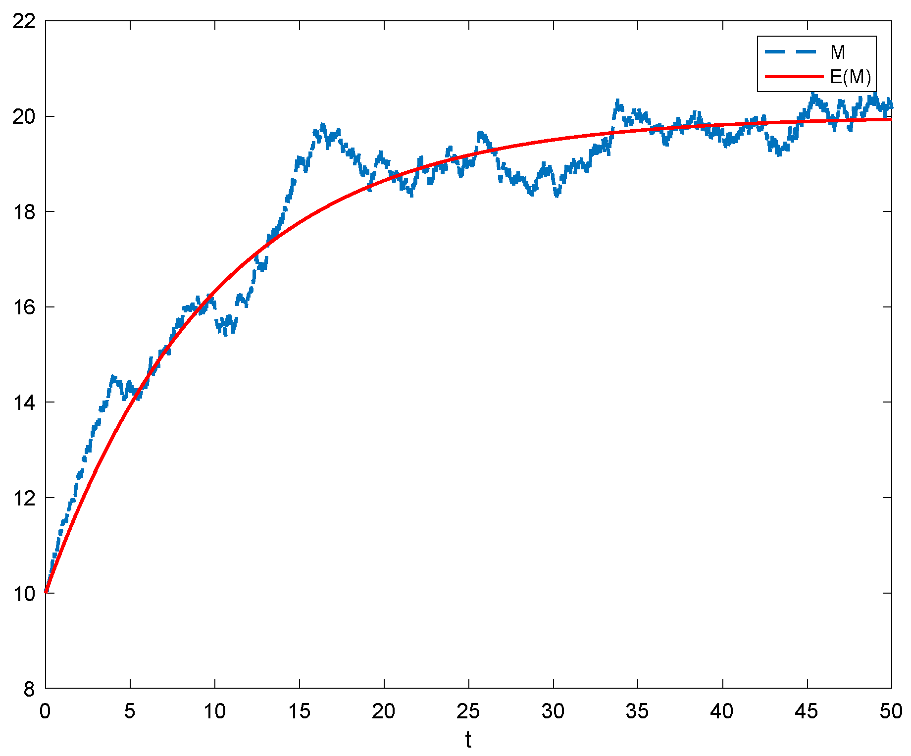
The relationship between the insured’s bad reputation record and its expected value is illustrated by simulation. The parameter values are set as follows: $M_0=10$, $\mathrm{\Delta }t=0.001$, ${\mathrm{O}}_1=4$, $\delta =0.01$, and $\sigma =1$; $\mathsf{\Phi }(t)$ is an independent and identically distributed standard normal distribution variable. Figure 1 shows the change in the policyholders’ bad reputation record process and their expected values over time without government regulation.

It can be seen from Figure 1 that, although bad reputation records are affected by random fluctuations, they always fluctuate around their expected value. Although we cannot accurately predict the evolution path of policyholders’ bad reputation records, we can use expectation and variance to estimate the possible interval size of bad reputation records. Assuming that bad reputation records follow a normal distribution, then, bad reputation records are below the confidence level of 95%, and the confidence interval for bad reputation records is: $\{E[M(t)]-1.96\sqrt{D[M(t)]},E[M(t)]+1.96\sqrt{D[M(t)]}\}$.

Thus, we conclude that, although the actual stock of bad reputation records may deviate from their expectations due to random factors, it is certain that, at a certain level of confidence, the bad reputation records of policyholders during the planning period remain within a certain range and fluctuate around their expectations. Extending this conclusion to motor vehicle insurance fraud management can bring important implications, i.e., when regulators cannot accurately grasp the bad reputation level of policyholders, if their expectations can be calculated, they can make corresponding decisions based on their expectations within the allowable range of errors.

3. Stochastic Differential Game Model under Government Supervision

Considering that, in the anti-fraud game of motor vehicle insurance, the government, as the highest regulator, supervises policyholders’ fraud and also supervises the work efforts of insurance companies. Therefore, we make the following assumptions on stochastic differential games under government supervision.

Hypothesis 5: 

Taking the cumulative amount of policyholders’ bad reputation records as a state variable, the degree of supervision by insurance companies and government departments and policyholder fraud as control variables, and taking into consideration the natural attenuation of bad reputation records, the process by which policyholders’ bad reputation records change over time becomes:

$$M^c(t)=[{\epsilon }_1{g}_1(t)u(t)+g_2(t)(1-{\epsilon }_1){\epsilon }_{2}u(t)-\delta M^c(t)]dt+\sigma [M^c(t)]d\omega (t)$$

(12)

Among them, $M^c(t)$ is the cumulative amount of bad reputation of policyholders under government supervision at time $t$; ${\epsilon }_2\in [0,1]$ is the regulatory success rate of government departments; $g_2(t)$ is the strength of government regulation at time $t$.

Hypothesis 6: 

There is a correlation between the regulatory costs of government departments and their regulatory efforts. Usually, as the degree of effort increases, the cost of effort also generally increases, but the increase in cost will tend to balance after reaching a certain threshold. Therefore, in this paper, we use a convex function to describe the relationship between the effort level of government departments and the effort cost. It is assumed that the effort cost of government departments is $\frac{b_3}{2}{g}_2{(t)}^2$, where $b_3$ is the regulatory cost coefficient of government departments.

Based on the above assumptions, we can obtain the revenue function of each participant.

Income function of the insured:

$${\displaystyle {\int }_0^t{e}^{-\rho t}}[Q_1+\alpha u(t)-\frac{b_1}{2}u{(t)}^2-(f+m)M^c(t)]dt$$

(13)

Income function of the insurance company:

$${\displaystyle {\int }_0^t{e}^{-\rho t}}\{Q_2-\alpha u(t)-\frac{b_2}{2}{g}_1{(t)}^2-{\epsilon }_2[T-g_1(t)]\omega +f{M}^c(t)\}dt$$

(14)

Income function of a government department:

$${\displaystyle {\int }_0^t{e}^{-\rho t}}[Q_3-\frac{b_3}{2}{g}_2{(t)}^2+{\epsilon }_2[T-g_1(t)]\omega +m{M}^c(t)]dt$$

(15)

Among them, $Q_3$ is the basic income of government departments and ${\epsilon }_2[T-g_1(t)]\omega$ is the government’s penalty for not trying hard to supervise the insurance company, $\omega >0$ is the penalty or penalty intensity, $T>0$ is the minimum supervision that the insurance company should have, $m>0$ represents the punishment coefficient of government departments to policyholders with bad reputations.

Theorem 4. 

Under government supervision, the optimal fraud intensity for an insured is:

$$u^{\ast \ast }=\frac{a{b}_2{b}_3-\frac{f+m}{\delta +\rho }{b}_3{\epsilon }_1{\epsilon }_2\omega }{b_1{b}_2{b}_3+\frac{(f+m)m}{{(\delta +\rho )}^2}{b}_2{\epsilon }_2^2{(1-{\epsilon }_1)}^2+\frac{(f+m)f}{{(\delta +\rho )}^2}{b}_3{\epsilon }_1^2}$$

(16)

Under government regulation, the optimal level of effort of an insurance company is:

$$g_1^{\ast \ast }=\frac{{\epsilon }_2\omega }{b_2}+\frac{{\epsilon }_1\frac{f}{\rho +\delta }(\alpha b_2{b}_3-\frac{f+m}{\rho +\delta }{b}_3{\epsilon }_1{\epsilon }_2\omega )}{b_1{b}_2^2{b}_3+\frac{(f+m)m}{{(\delta +\rho )}^2}{b}_2^2{\epsilon }_2^2{(1-{\epsilon }_1)}^2+\frac{(f+m)f}{{(\delta +\rho )}^2}{b}_3{b}_2{\epsilon }_1^2}$$

(17)

Under government supervision, the optimal level of effort of a government department is:

$$g_2^{\ast \ast }=\frac{(a{b}_2-\frac{f+m}{\delta +\rho }{\epsilon }_1{\epsilon }_2\omega )(1-{\epsilon }_1){\epsilon }_2\frac{m}{\rho +\delta }}{b_1{b}_2{b}_3+\frac{(f+m)m}{{(\delta +\rho )}^2}{b}_2{\epsilon }_2^2{(1-{\epsilon }_1)}^2+\frac{(f+m)f}{{(\delta +\rho )}^2}{b}_3{\epsilon }_1^2}$$

(18)

The proof is shown in Appendix C.

Theorem 5. 

Under government supervision, the optimal benefit for the insured is:

$$\begin{array}{l}{V}_u^c=\frac{-(f+m)}{\rho +\delta }{M}^c+\frac{1}{\rho }\{Q_1+\frac{\alpha b_2{b}_3(\rho +\delta )-(f+m)b_3{\epsilon }_1{\epsilon }_2\omega }{\mathrm{\Omega }}\\ \{\alpha -\frac{b_1}{2}\frac{\alpha b_2{b}_3(\rho +\delta )-(f+m)b_3{\epsilon }_1{\epsilon }_2\omega }{\mathrm{\Omega }}+\frac{-(f+m)}{\rho +\delta }\\ \frac{{\epsilon }_1{\epsilon }_2\omega +{\epsilon }_{1}f[\alpha b_2{b}_3(\rho +\delta )-(f+m)b_3{\epsilon }_1^2{\epsilon }_2\omega ]}{b_2\mathrm{\Omega }}\\ +\frac{-(f+m)}{\rho +\delta }\frac{[\alpha b_2(\rho +\delta )-(f+m){\epsilon }_1{\epsilon }_2\omega ]{(1-{\epsilon }_1)}^2{\epsilon }_2^{2}m}{\mathrm{\Omega }}]\}\}\end{array}$$

(19)

Under government supervision, the optimal benefits of insurance companies are:

$$\begin{array}{cc}\hfill & V_{g_1}^c=\frac{f}{\rho +\delta }M+\frac{1}{\rho }\{Q_2-\frac{{\alpha }^2{b}_2{b}_3(\rho +\delta )-\alpha (f+m)b_3{\epsilon }_1{\epsilon }_2\omega }{\mathrm{\Omega }}\hfill \\ \hfill & -{\epsilon }_{2}T\omega +\frac{{\epsilon }_2\omega +{\epsilon }_{1}f[\alpha b_2{b}_3(\rho +\delta )-(f+m)b_3{\epsilon }_1{\epsilon }_2\omega ]}{b_2\mathrm{\Omega }}\hfill \\ \hfill & \{-\frac{b_2}{2}\frac{{\epsilon }_2\omega +{\epsilon }_{1}f[\alpha b_2{b}_3(\rho +\delta )-(f+m)b_3{\epsilon }_1{\epsilon }_2\omega ]}{b_2\mathrm{\Omega }}+{\epsilon }_2\omega \hfill \\ \hfill & +\frac{f{\epsilon }_1}{\rho +\delta }\frac{\alpha b_2{b}_3(\rho +\delta )-(f+m)b_3{\epsilon }_1{\epsilon }_2\omega }{\mathrm{\Omega }}\}\hfill \\ \hfill & +\frac{f}{\rho +\delta }\frac{[a{b}_2(\rho +\delta )-(f+m){\epsilon }_1{\epsilon }_2\omega ]{(1-{\epsilon }_1)}^2{\epsilon }_2^{2}m}{\mathrm{\Omega }}\hfill \\ \hfill & \frac{\alpha b_2{b}_3(\rho +\delta )-(f+m)b_3{\epsilon }_1{\epsilon }_2\omega }{\mathrm{\Omega }}\}\hfill \end{array}$$

(20)

Under the supervision of the government, the optimal benefits of government departments are:

$$\begin{array}{cc}\hfill & V_{g_2}^c=\frac{m}{\rho +\delta }M+\frac{1}{\rho }\{Q_3+\hfill \\ \hfill & \frac{{\epsilon }_2\omega T{b}_2\mathrm{\Omega }-{\epsilon }_2^2{\omega }^2-{\epsilon }_2{\epsilon }_1\omega f[\alpha b_2{b}_3(\rho +\delta )-(f+m)b_3{\epsilon }_1{\epsilon }_2\omega ]}{b_2\mathrm{\Omega }}\hfill \\ \hfill & +\frac{m}{\rho +\delta }\frac{{\epsilon }_1{\epsilon }_2\omega +{\epsilon }_1^{2}f[\alpha b_2{b}_3(\rho +\delta )-(f+m)b_3{\epsilon }_1{\epsilon }_2\omega ]}{b_2\mathrm{\Omega }}\hfill \\ \hfill & \frac{\alpha b_2{b}_3(\rho +\delta )-(f+m)b_3{\epsilon }_1{\epsilon }_2\omega }{\mathrm{\Omega }}\hfill \\ \hfill & +\frac{[a{b}_2(\rho +\delta )-(f+m){\epsilon }_1{\epsilon }_2\omega ](1-{\epsilon }_1){\epsilon }_{2}m}{\mathrm{\Omega }}\hfill \\ \hfill & \{-\frac{b_2}{2}\frac{[a{b}_2(\rho +\delta )-(f+m){\epsilon }_1{\epsilon }_2\omega ](1-{\epsilon }_1){\epsilon }_{2}m}{\mathrm{\Omega }}+\hfill \\ \hfill & \frac{m}{\rho +\delta }(1-{\epsilon }_1){\epsilon }_2\frac{\alpha b_2{b}_3(\rho +\delta )-(f+m)b_3{\epsilon }_1{\epsilon }_2\omega }{\mathrm{\Omega }}\}\}\hfill \end{array}$$

(21)

The proof process of Theorem 5 is the same as that of Theorem 2 in Section 2, which we omit here, due to space limitations.

Theorem 6. 

Under government supervision, the insured’s bad reputation record expectations and stability values are: $E[M^c(t)]=\frac{{\mathrm{O}}_2}{\delta }+e^{-\delta t}(M_0^c-\frac{{\mathrm{O}}_2}{\delta })$,$\underset{t\to +\infty }{\lim }E[M^c(t)]=\frac{{\mathrm{O}}_2}{\delta }$. The variance values and their stable values for the policyholders’ bad reputation records are: $D[M^c(t)]=\frac{{\sigma }^2[{\mathrm{O}}_2-2({\mathrm{O}}_2-\delta M_0^c)e^{-\delta t}+({\mathrm{O}}_1-2\delta M_0^c)e^{-2\delta t}]}{2{\delta }^2}$,$\underset{t\to +\infty }{\lim }D[M^c(t)]=\frac{{\sigma }^2{\mathrm{O}}_2}{2{\delta }^2}$, where,

$$\begin{array}{l}{\mathrm{O}}_1=\frac{\alpha b_2{b}_3(\rho +\delta )-(f+m)b_3{\epsilon }_1{\epsilon }_2\omega }{\mathrm{\Omega }}\{\frac{{\epsilon }_1{\epsilon }_2\omega +{\epsilon }_1^{2}f[\alpha b_2{b}_3(\rho +\delta )-(f+m)b_3{\epsilon }_1{\epsilon }_2\omega ]}{b_2\mathrm{\Omega }}\\ +\frac{[a{b}_2(\rho +\delta )-(f+m){\epsilon }_1{\epsilon }_2\omega ]{(1-{\epsilon }_1)}^2{\epsilon }_2^{2}m}{\mathrm{\Omega }}\}\end{array}$$

The proof process of Theorem 6 is the same as that of Theorem 3 in Section 2, which we have omitted here, due to space limitations.

4. Simulation Analysis

In this paper, we assume that the parameters $\alpha =40$, ${\epsilon }_1={\epsilon }_2=0.5$, $f=6$, $m=4$, $b_1=b_3=2$, $b_2=1$, $\delta =0.5$, $\rho =0.1$, and $\omega =3$ satisfy $u\ge 0,g_1\ge 0,g_2\ge 0$. The system is simulated by MATLAB 2018a, and the influence of each parameter on the participant selection strategy is obtained.

4.1. The Influence of Initial Value on the Optimal Trajectory of Bad Reputation Record Stock

Let the initial value $M_0$ of the enterprise’s bad reputation record stock be 0 and 40, and other parameters remain unchanged. The changes of the optimal trajectory of the bad reputation record stock under different initial values with or without government supervision are discussed.

As can be seen from Figure 2, although there are random factors that cause the actual trajectory of bad reputation records to fluctuate to a certain extent, they all fluctuate up and down around their expected values. By observing the expectations of each situation, it can be found that regardless of whether there is government supervision or not, although the stock state reached by different initial values after a long period of evolution is the same, their evolution paths are different. For policyholders with higher initial values, the stock of bad reputation gradually decreases in the short term and eventually stabilizes. This can be understood as when the initial bad reputation of the fraudulent insured is high, due to the higher punishment, and thus, restrained by the pressure of punishment, the intensity of fraud decreases until the insured’s marginal cost of fraud is reduced to equal to the marginal benefit of fraud, reaching a final stable state. For policyholders with low initial values, the stock of bad reputation gradually increases in the short term, and eventually tends to stabilize. This situation can be understood as, when policyholders’ bad reputation is small, due to lighter punishment, they can not withstand the temptation of high fraudulent profits and continue some fraudulent acts. However, as the stock of bad reputation records increases, policyholders are increasingly punished. When the marginal cost of policyholders’ fraud increases to the same marginal benefit of fraud, policyholders will abandon the fraud, thus, achieving a zero-growth rate of bad reputation records per unit time. By comparing Figure 2a,b, we can find that, at the same initial value, the stable value of the stock of bad reputation records of policyholders with government regulation is less than that in the absence of government supervision. This can be understood as, when the government departments join the game, policyholders are subject to punishment from the government under the same stock of bad reputation records. Therefore, the original balance between the marginal cost of fraud and the marginal benefit of fraud is broken. Therefore, the insured needs to reduce the intensity of fraud, thereby, reducing the disciplinary impact of the bad reputation record stock, and once again reaching a balanced state.

4.2. Influence of Natural Attenuation Rate $\delta$ on Equilibrium Solution of Game Participants

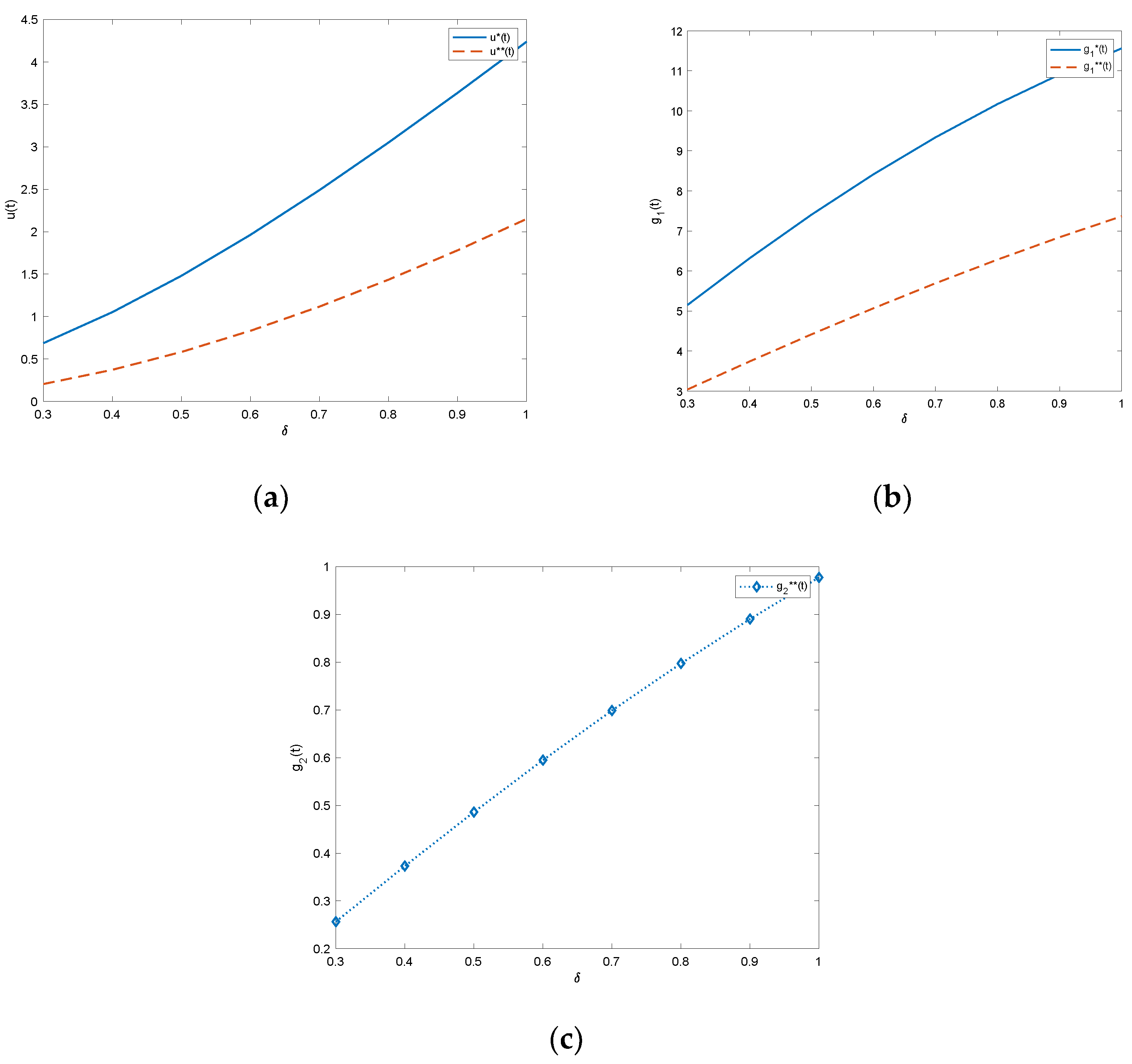
In order to facilitate the observation of the influence of natural decay rate on the game, in this paper, we set the natural decay rate of bad reputation record in the interval [0.3,1], while other parameters remain unchanged, and we discuss the influence of natural decay rate on the equilibrium solution of the players in the game with or without government supervision. The results are shown in Figure 3. Figure 3a shows the change in the optimal fraud intensity of the insured at different natural decay rates, Figure 3b shows the change in the optimal effort degree of the insurance company at different natural decay rates, and Figure 3c shows the change in the optimal effort of the government department at different natural decay rates.

As can be seen from Figure 3a, the intensity of fraud by policyholders is positively correlated with the natural decay rate of bad reputation records, regardless of whether there is government regulation; as the natural decay rate increases, the fraud intensity of policyholders increases and the fraud intensity of policyholders with government supervision is significantly smaller than that of policyholders without government supervision. Similarly, according to Figure 3b,c, it can also be observed that the optimal effort of insurance companies and the optimal effort of government departments are positively correlated with the natural decay rate, which increases as the natural decay rate increases.

The greater the rate of natural decay, the faster the rate of natural decay of bad reputation records without taking into account the behavioral strategies of policyholders, insurance companies, and government departments. This means that in a short period of time, the stock of bad reputation records can be reduced, so that the penalty for the insured is reduced, thereby, reducing the cost of fraud of the insured, and the insured chooses to increase the intensity of fraud in order to obtain more benefits. At this time, rational insurance companies and government departments must strengthen their own supervision to effectively restrain the fraud intensity of policyholders.

4.3. Influence of Punishment Strength $f$, $m$, $\omega$ on Equilibrium Solution of Game Participants

By keeping other parameters unchanged and setting the value ranges of disciplinary intensity $f$, $m$, and $\omega$ to be [0.05,20], [0.05,20], [1,6], respectively, we can observe the impact of disciplinary intensity on the equilibrium solution of policyholders, insurance companies, and government departments. The results are shown in Figure 4.

Figure 4a shows the influence of punishment intensity $f$ on the equilibrium solution of policyholders and insurance companies under the condition of no government supervision. Figure 4b shows the influence of punishment intensity $f$ on the equilibrium solution of policyholders, insurance companies, and government departments under the condition of government supervision. Figure 4c shows the influence of punishment intensity $m$ on the equilibrium solution of policyholders, insurance companies, and government departments under the condition of government supervision. Figure 4d shows the influence of punishment intensity $\omega$ on the equilibrium solution of policyholders, insurance companies, and government departments under the condition of government supervision.

According to Figure 4a, under the condition of no government supervision, with an increase in punishment intensity $f$, the fraud intensity of the insured gradually decreases, while the supervision intensity of the insurance company has a trend of increasing first and then decreasing. This situation can be explained by the fact that, with an increase in the intensity of punishment, the insured is restricted by disciplinary pressure, and therefore, there is a gradual reduction in fraud intensity. When the punishment intensity is small, the fraud intensity of the insured is larger, and the amount of insurance company fraud claims for loss increases, and therefore, the insurance company chooses to increase the intensity of supervision. With an increase in punishment, the insured reduces the intensity of fraud. When the insured reduction in the intensity of fraud is greater than the intensity of punishment $f$, the insurance company will gradually reduce the intensity of supervision. According to Figure 4b, under the condition of government supervision, with an increase in punishment intensity $f$, the fraud intensity of applicants gradually decreases, and the supervision intensity of the government also shows a gradual decline, while the supervision intensity of the insurance company first increases and then decreases. According to Formula (A33), when the remaining parameters are unchanged, the supervision intensity of government departments is proportional to policyholders’ fraud intensity. Therefore, as policyholders’ fraud intensity increases, the supervision intensity of government departments shows a growing trend. According to Figure 4c, with an increase in disciplinary intensity $m$, the policyholders’ fraud intensity decreases, the supervision intensity of insurance companies gradually decreases, and the supervision intensity of government departments gradually increases. According to Formula (A32), it can be shown that when the remaining parameters remain unchanged, the supervision of the insurance company is positively correlated with the intensity of the insured’s fraud, and therefore, the intensity of the insured’s fraud decreases, and the supervision of the insurance company also decreases. According to Formulas (A33) and (A48) it can be shown that when the degree of the insured’s reduction in fraud intensity is less than the intensity of punishment $m$, the government department will gradually increase the intensity of supervision. According to Figure 4c, with an increase in punishment intensity, policyholders’ fraud intensity and the supervision intensity of the government department show a downward trend, while the supervision intensity of the insurance company shows an upward trend. Because the penalties $\omega$ are used to constraint the insurance company, with an increase in $\omega$, it forces a a higher degree of supervision by insurance companies; the supervision intensity of the insurance company increases and limits the increase in policyholders’ fraud intensity. When the other parameters are the same, government regulation is positively related to the intensity of policyholders’ fraud, therefore, with the strength of policyholders’ fraud is reduced, and government oversight also declines.

Through the above analysis, insurance companies and government departments should appropriately increase the intensity of punishment according to the actual situation, and force the insured to reduce fraud intensity under the pressure of punishment until fraud is no longer committed.

4.4. The Impact of Regulatory Success Rates on the Intensity of Fraud by Policyholders

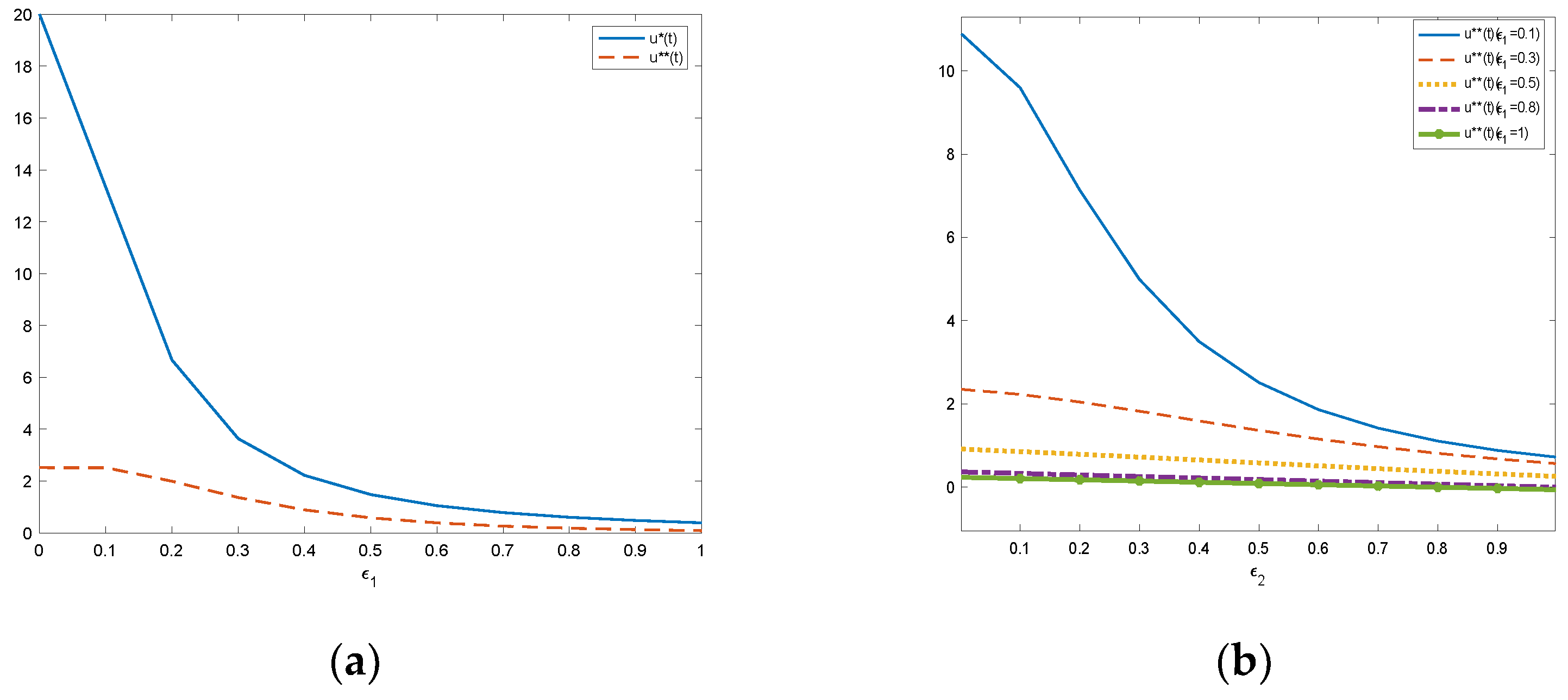
In this article, mainly through an analysis of the reputation of policyholders, bad reputation policyholders respond to a certain degree of punishment, in order to achieve effective governance of policyholder fraud. Therefore, in this section, we mainly study the impact of regulatory success rate on the fraud intensity of policyholders. Let the regulatory success rate of insurance companies and government departments change between [0,1] and keep the remaining parameters unchanged, we discuss the change of the optimal fraud intensity of the insured under different regulatory success rates. Figure 5a shows the impact of the success rate of insurance company supervision on the fraud intensity of policyholders with or without government supervision. Figure 5b shows the impact of changing the success rate of government supervision on the fraud intensity of policyholders when the success rate of insurance company supervision is 0.1, 0.3, 0.5, 0.8, and 1.

According to Figure 5, as the regulatory success rate of insurance companies or government departments increases, the fraud intensity of policyholders gradually decreases. The greater the success rate of supervision, the greater the probability that the insured’s fraud will be found, and the higher the punishment of the insured will be. Therefore, rational policyholders will choose to reduce their fraud intensity to reduce the cost of punishment. Through Figure 5a, we can find that under the same regulatory success rate of insurance companies, the fraud intensity of policyholders with government supervision is generally lower than that without government supervision. Through Figure 5b, it can be seen that when the success rate of government supervision is unchanged, with an increase in the success rate of insurance company supervision, the fraud intensity of policyholders gradually decreases. When the success rate of insurance company supervision is fixed, with an increase in the success rate of government supervision, the fraud intensity of policyholders gradually decreases. Based on the above analysis, it is concluded that insurance companies and government departments can effectively reduce the fraud intensity of policyholders by improving the success rate of supervision of dishonest policyholders until fraud no longer occurs.

5. Summary

In this paper, a stochastic differential game model is constructed with the goal of maximizing the income of the participants in the motor vehicle insurance anti-fraud game, and the bad reputation of the policyholder caused by fraud is taken into account, in order to achieve the purpose of not cheating by punishing, to a certain extent, the policyholder with a bad reputation. In this paper, the feedback equilibrium solution of the participants is obtained by using an analytical method, and the influence of each important parameter on the equilibrium solution is analyzed by simulation. Through analysis and simulation, we can draw the following conclusions: (1) Compared with the case without government supervision, in the case of government supervision, the fraud intensity of the insured is smaller, which is more conducive to curbing the fraud intensity of the insured. (2) The policyholders with higher bad reputation will reduce their stock of bad reputation records by reducing the intensity of fraud, while the policyholders with lower bad reputation will increase their stock of bad reputation in the short term, and eventually the two will converge at the same level. (3) Increasing the intensity of punishment can increase the cost of dishonesty of the insured, making the insured under the pressure of punishment reduce the intensity of their own fraud. (4) Improving the success rate of fraud supervision can lead to an increase in the probability that the insured’s fraud is found, thereby, increasing the cost of fraud punishment. Therefore, the insured reduces its fraud intensity as the success rate of insurance company/government supervision increases until no fraud is committed.