Article

Unraveling the Most Influential Determinants of Residential Segregation in Jakarta: A Spatial Agent-Based Modeling and Simulation Approach

School of Business and Management, Institut Teknologi Bandung, Jl. Ganesa 10, Bandung 40132, Indonesia
*
Author to whom correspondence should be addressed.
Systems 2023, 11(1), 20; https://doi.org/10.3390/systems11010020
Submission received: 23 November 2022 / Revised: 20 December 2022 / Accepted: 30 December 2022 / Published: 2 January 2023

Abstract

:
This study involves the analysis of the residential segregation patterns in Jakarta, Indonesia, one of the largest global metropolitan cities. Our objective is to determine whether similarities in religion or socioeconomic status are more dominant in shaping residential segregation patterns in Jakarta. To do so, we extended Schelling’s segregation agent-based model incorporating the random discrete utility choice approach to simulate the relocation decisions of the inhabitants. Utilizing actual census data from the 2010–2013 time period and the Jakarta GIS map, we simulated the relocation movements of the inhabitants at the subdistrict level. We set the inhabitants’ socioeconomic and religious similarities as the independent variables and the housing constraints as the moderating variable. The segregation parameters of the inhabitants (i.e., dissimilarity and Simpson indexes) and the spatial patterns of residential segregation (i.e., Moran index and segregation maps) were set as the dependent variables. Additionally, we further validated the simulation outcomes for various scenarios and contrasted them with their actual empirical values. This study concludes that religious similarity is more dominant than socioeconomic status similarity in shaping residential segregation patterns in Jakarta.

1. Introduction

The segregation phenomenon has gained the attention of social researchers, considering residential segregation as a fundamental characteristic of modern cities [1]. Timberlake [2] defines residential segregation as the spatial separation of several social groups within a particular geographic area. Typically, more heterogeneous groups of people inhabit cities compared with rural areas. This heterogeneity is associated with an uneven population distribution in urban spaces, leading to certain residential segregation patterns [3]. Furthermore, residential segregation influences numerous aspects of life [4], such as access to transportation [5], education [6], job opportunities [7], and health services [8].
Several factors contribute to population heterogeneity, e.g., race/ethnicity, gender, religion, socioeconomic status, language, etc. These factors can motivate an individual in deciding her place of residence [8,9,10,11,12]. This fact is understandable, given the definition of segregation, which also connotes inequality [13]. As a source of urban problems, segregation, in the form of income inequality, has become a central theme for researchers in understanding the relationship between socioeconomic aspects and spatial patterns in settlements [14,15,16]. In many cases, the interplay between socioeconomic characteristics and the basic property of inhabitants (e.g., race, ethnicity, and religion) manifests in a clear residential segregation pattern [12].
Studies on segregation mostly use descriptive approaches in analyzing the clustering phenomenon in the people’s choice of residency [5,14,15,16,17,18,19,20,21]. However, few studies scrutinize inhabitants’ internal motivation and the reasons for their choice of residency. It is challenging for a study to ask individuals why they choose to live in a specific place, especially if the reasons relate to sensitive matters such as race, religion, etc. Research methods, such as surveys and in-depth interviews, have their limitations. To overcome this, an alternative research approach is required to analyze the driving factors behind residential segregation and verify the findings with real-time empirical demographic data.
Agent-based modeling (ABM) is a computational approach that enables a detailed analysis of the system’s behavior at an individual agent level [22]. The agents in ABM act autonomously based on a set of behavioral rules, producing emergent collective behaviors [23]. One of the earliest studies analyzing segregation using ABM is Schelling’s “Dynamic Models of Segregation” [24]. In the original Schelling model, agents decide to move or stay in a place based on the percentage of dissimilarity they can tolerate in their neighborhood, represented by the agent’s threshold value [24]. We extended this simple mechanism by applying a random utility discrete choice approach as the basis for the relocation decision of each agent [25].
As a case study, we focused on the analysis of segregation in Jakarta Province (Figure 1), a multidimensional, diverse metropolitan area in Indonesia. Jakarta has an area of 664.01 square kilometers with a population of 10,562,088. Consisting of five administrative municipalities, Jakarta is one of the most heterogeneous provinces in Indonesia. Its residents include several ethnic groups such as Javanese (36.17%), Betawi (28.29%), Sundanese (14.61%), Chinese (6.62%), Batak (3.42%), Minangkabau (2.85%), Malay (0.96%), and others (7.08%) [26].
Previous studies on residential segregation in Jakarta concluded that the socioeconomic factor is the primary driver of population segregation [11,20,27]. This study challenges previous research findings by scrutinizing the aspect of religious similarity in the analysis. Specifically, we sought to determine whether similarities in religion or socioeconomic status are more dominant in shaping spatial segregation patterns.

2. Literature Review

Schelling [24] concluded that segregation can arise through mild preferences of agents in choosing their place of residency based on demographic or socioeconomic similarities. Previous studies have identified the influence of demographic elements such as race [28], ethnicity [29], sex [30], or age group [31] on individual residential preferences in shaping residential segregation patterns. Some studies have also explored cultural characteristics, such as language [18] and religion [32]. Recently, studies investigating the socioeconomic aspect as the driver of segregation have also become more popular. These studies aimed to find the root of socioeconomic problems by analyzing the inhabitants’ spatial footprint [14,16,33].
Ethnicity has also been identified as a dominant driver of segregation [8,29,31,34,35]. Ethnic identity is an attribute that individuals attain through inheritance, although, in some instances, ethnic switching occurs due to marriage [19]. Earlier studies found that ethnic segregation can occur in schools [36], workplaces [37], or neighborhoods [38]. Specific ethnic compositions that result in the presence of minority groups contribute to the emergence of segregation. With computational approaches, researchers have successfully visualized this ethnic composition into observable patterns [15,39,40,41].
To the best of our knowledge, religious preferences have been less addressed in the literature. Merino [10] reported that, although scholars believe religion contributes significantly to segregation in the United States, no one has provided solid evidence. Meanwhile, Fong et al. [32] conducted a statistical analysis to examine residential patterns among religious groups in Canada. They concluded that religious institutional behaviors, such as the institutional orientation of religious community services, subcultural identity, religious identity, and discrimination, influence segregation patterns [32].
The socioeconomic aspect has garnered the highest level of attention in the literature related to segregation [12,14,20]. The segregation process will always have implications for the social and economic conditions of a region. Segregation studies are essential in unraveling classic social issues in the urban area such as poverty and economic growth [20]. Policymakers can take advantage of the recommendations derived from research on segregation to improve urban planning policies. The act of physically destroying slum areas to reduce segregation, for example, does not solve the root cause of the problem; instead, it only redistributes poverty throughout the city [14].
Table 1 provides an overview of the previous studies related to the driving factors of segregation. In general, many studies focused on a singular aspect of segregation, namely ethnic/race, religion, or socioeconomic status only. Those studies applied either statistical, spatial, or agent-based modeling in analyzing segregations in different regions such as America, Australia, Brazil, the UK, etc. [17,20,42]. This study complements this body of research by analyzing two segregation determinants simultaneously, namely religion and socioeconomic dissimilarity aspects, using agent-based modeling and simulation.

3. Case Study: Jakarta

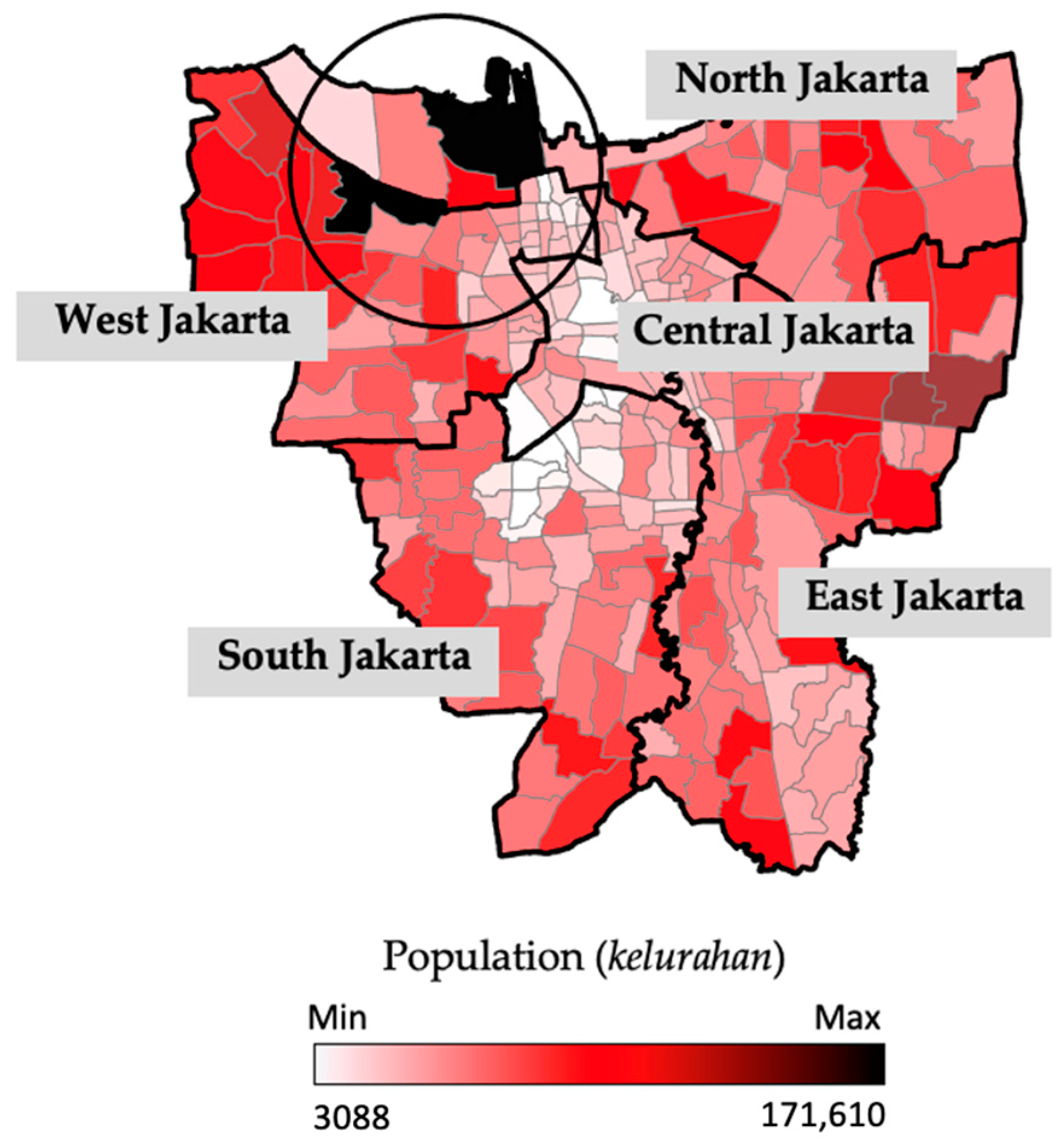
As a case study, we focused on analyzing the segregation phenomenon in Jakarta, the capital of Indonesia. Jakarta consists of six administrative regencies: North Jakarta, East Jakarta, South Jakarta, West Jakarta, Central Jakarta, and Kepulauan Seribu. We excluded the Kepulauan Seribu regency since it is located on other islands, not on the mainland; thus, residents’ relocation across the sea is less likely. The 5 analyzed administrative regencies consist of 261 subdistricts (kelurahan) (Figure 2). A kelurahan, the smallest geographical region in our simulation model, has an average area of 2.5 square kilometers with 15,907 inhabitants per square km. North Jakarta consists of 30 kelurahans; East Jakarta consists of 65 kelurahans, South Jakarta has 65 kelurahans, Central Jakarta has 44 kelurahans, and West Jakarta consists of 56 kelurahans. In our study, relocation occurs when the inhabitant moves residency between different kelurahans.
Jakarta is inhabited by more than 10.56 million people [43]. Figure 2 illustrates the population density of Jakarta. As shown, the population is higher in the peripheral areas farther from the city center. Areas with low population density (Central Jakarta, parts of South Jakarta, and parts of West Jakarta) are dominated by office buildings and malls, which are hubs of commercial activities but are not considered residential. The black region in the circle highlights the two most populated kelurahans.

3.1. The Religion Spatial Pattern

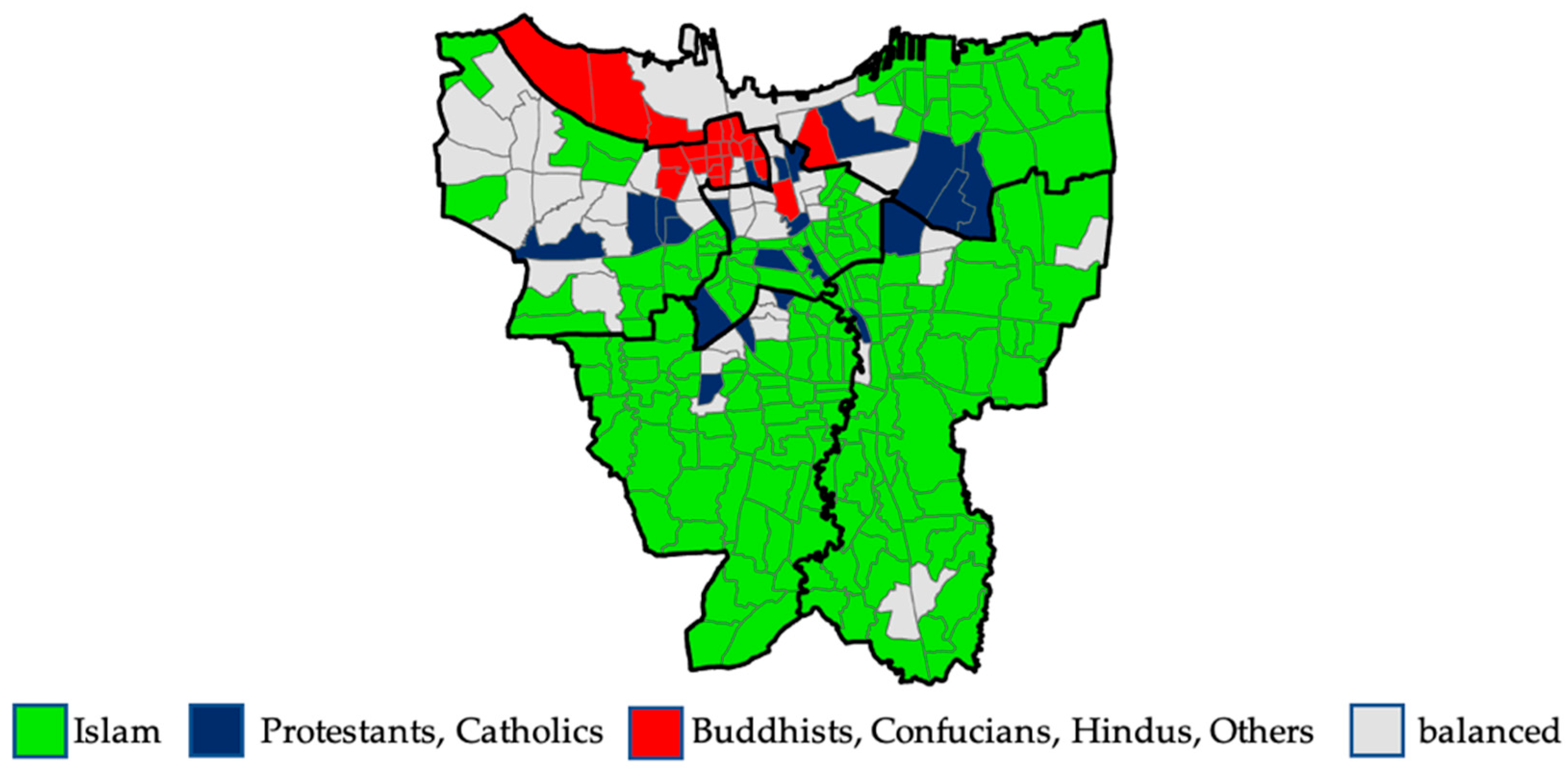
Figure 3 reveals the spatial pattern of the dominating religion for each kelurahan. The green area indicates kelurahans with the highest Muslim population. The population concentration of Protestants and Catholics is high in the blue areas, while the red area is an area of concentration of Buddhists, Confucians, Hindus, and Others. As can be seen, the red-colored kelurahans are located close to each other. The green-colored regions also tend to be close to one another. This spatial pattern indicates an early symptom of residential segregation driven by religious similarity.
To reduce the computational load of the agent-based simulation, we grouped the actual seven categories of religions into three clusters, namely Muslims, Christians, and others. We conducted the clustering based on two considerations: (1) the magnitude of the followers of these religions individually and (2) the correlation analysis among the followers of different religions (Table 2). The first group is Muslim, which is the majority in Jakarta (83.4%). For the second group, the Protestant and Catholic populations had a high correlation value (0.799), and we grouped them as Christians. We categorized the remaining religious groups as “others”.

3.2. The Socioeconomic Spatial Pattern

Previous studies used the data on the occupation of residents as a reference for their socioeconomic status [16,20]. However, the Jakarta census data classify occupations into 88 types of professions. This high number of occupation variants leads to a computational challenge in simulating and comprehensively interpreting the segregation pattern. Thus, we considered educational level as a proxy for an individual’s socioeconomic status [44]. For the simulation, we then codified the educational levels as follows: not completed elementary school (LOW), graduated elementary and junior high school (MIDDLE), and graduated high school (HIGH).
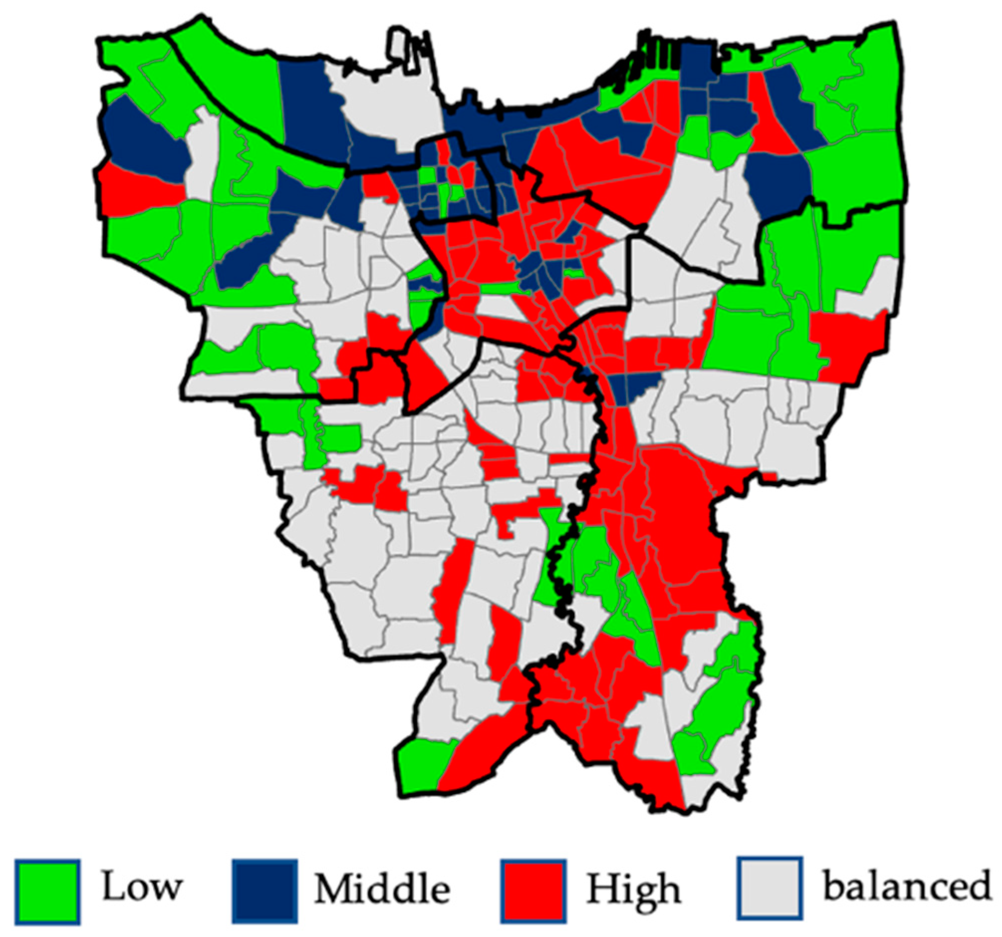
In contrast to the religious concentration map, the spatial pattern of Jakarta’s population based on SES shows a more diverged pattern (Figure 4). Low SES dominates the green area. The blue area is the population concentration with middle SES, while the red area shows the population with high SES. This spatial pattern indicates that the population with high SES is distributed along the central region from south to north. Additionally, it can be inferred from Figure 4 that the middle SES group is concentrated in the northern part, while the low SES group is distributed evenly in each region.
The map based on religious concentration (Figure 3) indicates clear zones among population clusters. By contrast, the spatial pattern maps based on SES show more moderate cluster boundaries. This visual difference leads to the conjecture that socioeconomic status does not contribute to segregation. Nevertheless, further investigation is required to clarify this hypothesis.

4. Conceptual Research Model

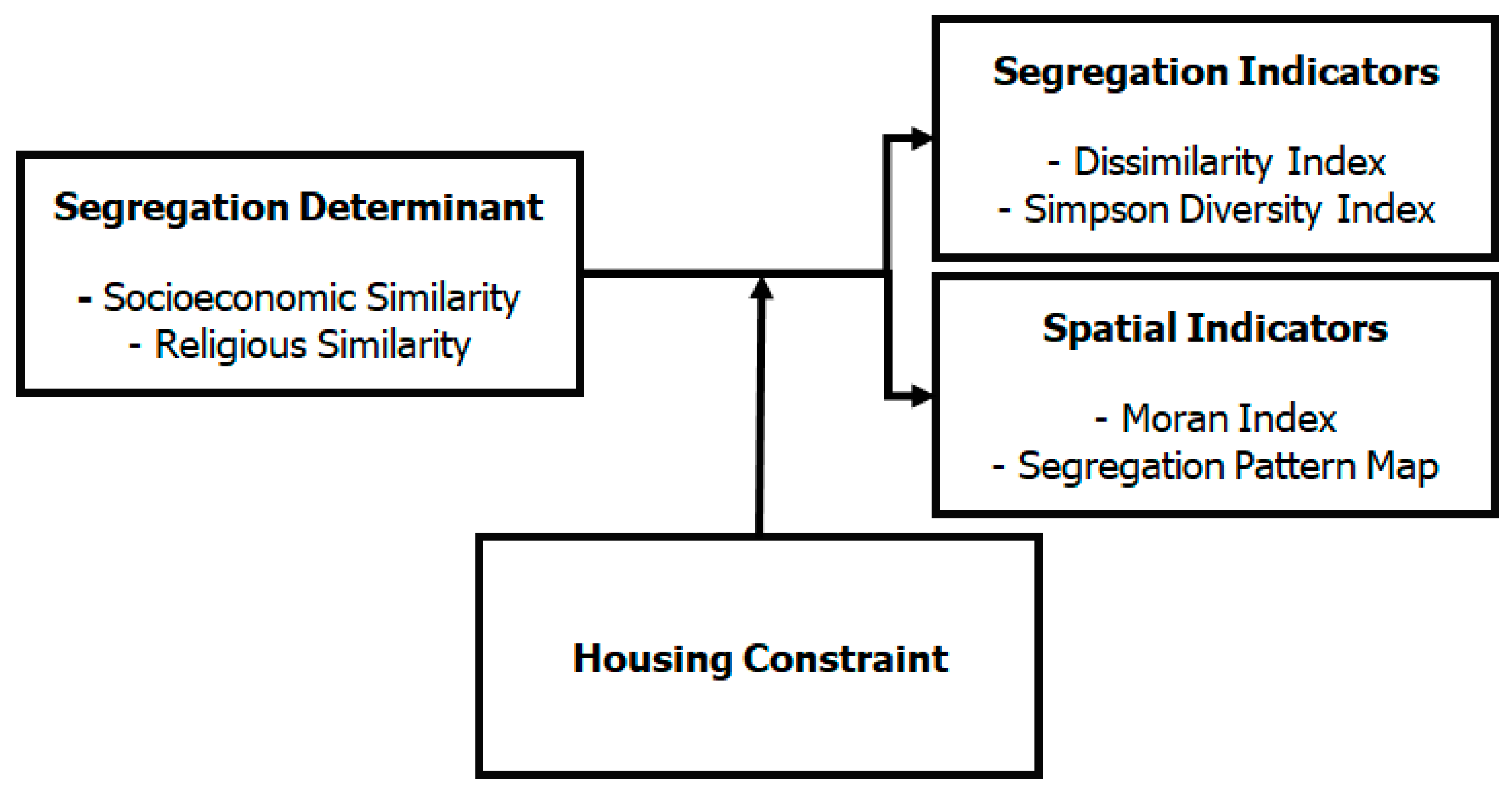
Figure 5 presents the conceptual model of this study. We applied ABM to determine whether socioeconomic or religious similarities are more influential on residential segregation in Jakarta. In the simulation, we used socioeconomic status similarity ( β S E S ) and religious similarity ( β r e l ) indexes as independent variables. We treated the housing constraints as the moderating variable. As a dependent variable, we assessed the level of segregation using the dissimilarity index, spatial correlation, and spatial pattern map. The level of segregation was assessed using qualitative and quantitative criteria. Qualitatively, we used a spatial pattern map and assessed the ABM simulation results of which of the two scenarios produce a more coherent spatial pattern between the actual empirical situation and the simulation results. Quantitatively, we assessed which ABM simulation scenario produces the least difference in the dissimilarity index and the spatial correlations between the actual empirical data and the simulation results.

4.1. Independent Variables

4.1.1. Weight of Similarity

In our model, each agent (i.e., an inhabitant) can decide to move to its neighboring kelurahan for each time step. The decision consists of two phases: searching and moving. In the searching phase, the agent evaluates the utility value of its current residence. If the utility value is positive, the agent will stay and ignore the second phase. If the utility value is negative, the agent will proceed to the second phase. In the second phase, the agent will compare its current utility value with the proposed utility value of a random prospective neighboring area. If the utility value of the neighboring area is better than its current utility value, the agent will relocate to the new area. Otherwise, the agent will stay at their current residence.
Adopting the discrete choice model [45], we formalized the agent’s utility value as follows:
u a b = μ a b + ε a b
where μ a b is all the (weighted) observable characteristics of neighborhood b , interacting with the attributes of agent a , and ε a b as the term for random error. We refined Equation (1) into two new equations to model the expected interactions in the predefined two scenarios. In the first scenario, we incorporated the interaction between ethnicity and SES in the utility function. The utility function was formalized as follows:
U X , Y , θ i = β E t h P i X θ + β S E S P i Y θ + ε
In the second scenario, we incorporated the interaction between ethnicity and religion in the utility function. The utility function was formalized as follows:
U X , Y , θ i = β E t h P i X θ + β r e l P i Y θ + ε
where X denotes ethnicity; Y denotes socioeconomic status/religion; θ is an agent’s threshold value which quantifies the minimum fraction of neighbors having similar properties that must be satisfied for an agent to stay at its current location; P i X denotes the fraction of the population with the same ethnicity; P i Y denotes the fraction of the population with the same socioeconomic status (i.e., Equation (2)) or the same religion (i.e., Equation (3)). The β E t h , β S E S , and β r e l represent the weights for similarity in ethnicity, socioeconomic status, and religion. The notation ε stands for the unobservable motives, i.e., the utility of the agent [45,46].
An agent moves to kelurahan j when U X , Y , θ j > U X , Y , θ i leaves an open place in the origin area (kelurahan i). The utility increases linearly in both P i X and P i Y so that high similarity on socioeconomic or religion can compensate for low ethnic similarity and vice versa. The unobservable utility factor of ε denotes all the unknown factors that affect an agent’s preference. The model will automatically add a random value ε from the standard Gumbel distribution1 to the total utility value. The effect of this random value will be greater if the value of β E t h , β S E S , or β r e l is low.

4.1.2. Housing Constraints

In the real world, people do not randomly opt for a place of residency. An agent’s decision of where to live is driven by certain considerations. The agent’s intention to choose a place to live economically is captured in scenario 1 of the simulation (i.e., SES preference). Scenario 2 represents the agent’s intention to stay in housing areas with inhabitants having a similar religion.
As shown in Figure 6, the agent decides to relocate to a new location when U X , Y , θ i < 0 . In each time step, the agent selects potential kelurahan  j , based on a random probability proportional to the number of vacant residences. If the housing constraints parameter is activated (i.e., on), the model will track all the trajectory locations of the agents based on SES or the religion practiced in the region. For example, a high-SES agent will only relocate to a region with similar socioeconomic status to the agent’s previous residency, i.e., one with high SES. When the housing constraints parameter related to religion is considered, an agent will only relocate to a region where the majority of the inhabitants have the same religion as the agent.

4.2. Dependent Variables

4.2.1. Segregation Indicators

Dissimilarity Index

The distribution of two groups over the smaller geographic regions (kelurahan as census tract) that make up a larger area is measured by the dissimilarity index (D). This variable is the ratio of the minority population to the majority population across all geographic locations [47]. The dissimilarity index is formalized as follows:
D = i = 1 n t i p i P 2 T P 1 P
where t i is the total population of area i , p i is the minority proportion of areal i , T is the total population, P is the minority proportion of the whole city, and n is the number of areas (census tracts) in the study area, which, in this study, refers to the number of kelurahan in Jakarta.

Simpson Index

The Simpson index ( λ ) is a measure of ethnic diversity. It can be viewed as an index of concentration reflecting the probability that two agents selected by random chance have a similar property (i.e., ethnic, religious, or socioeconomic property) [48]. The Simpson index ( λ ) is formalized as follows:
λ = i = 1 R p i 2
where p i is the fraction of the population of the i th type in the dataset, and R denotes the total number of groups (i.e., ethnic, religion, or socioeconomic property).

4.2.2. Spatial Indicators

Moran Index

The Moran index (Moran’s I) refers to the spatial autocorrelation across regions. It indicates whether the concentration of agents having similar properties exists. The index value ranges from −1 to 1, where −1 is the perfect clustering of distinct values (dispersed), 0 is no autocorrelation (perfect randomness), and 1 is the perfect clustering of similar values (clustered) [49]. The Moran index is formalized as follows [50]:
I = n W i = 1 n j = 1 n w i j x i X ¯ ( x j X ¯ ) i = 1 n x i X ¯ 2
where n is the number of objects in space; X ¯ is a mean value of an attribute; x i and x j are the values of an attribute for objects i and j ; w is a spatial weight for a pair of objects, and W is the sum of spatial weights.

Segregation Pattern Map

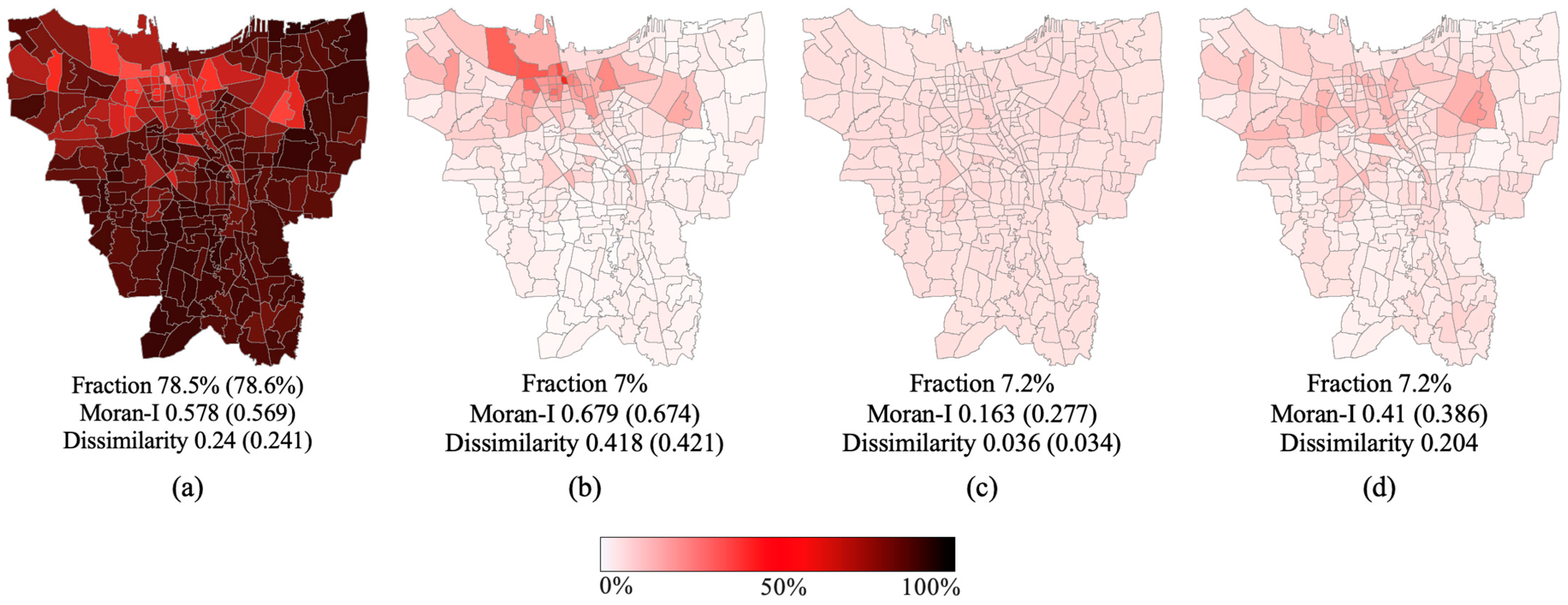
Figure 7 shows all the segregation pattern maps for each ethnicity, namely Javanese (EGJ), Sumatrans (EGS), Chinese, and other ethnicities. Notably, we used the actual empirical data to produce the plots and calculated the corresponding parameters such as Moran’s I and dissimilarity indexes. For each index, we determined two values, the first one complies with the ethnicity–SES scenario and the second one (i.e., the value inside the parentheses) complies with the ethnicity–religion scenario. As is evident, the inhabitants with Sumatran ethnicities (EGS) contributed to 7.2% of the total population with a Moran index value of 0.163 (0.277) and an ethnic dissimilarity index value of 0.036 (0.034). The inhabitants with Javanese ethnicities (EGJ) constitute 78.5% of the total population with a Moran index value of 0.578 (0.569) and an ethnic dissimilarity index value of 0.24 (0.241). The inhabitants with Chinese ethnicities comprised 7% of the total population with a Moran index value of 0.679 (0.674) and an ethnic dissimilarity index value of 0.418 (0.421).
Figure 7c shows that the inhabitants with Sumatran ethnicities (EGS) had the lowest value of dissimilarity (0.036 (0.034)) and Moran index (0.163 (0.277)). These values indicate that Sumatran ethnicities had the highest population dispersion in the region and the lowest level of preference for residing in a place with similar ethnic background. In contrast, the inhabitants with Chinese ethnicities had the highest value of dissimilarity (0.679 (0.674)) and Moran I index (0.418 (0.421)). These values indicate that Chinese ethnicities had the highest population concentration in the region and the highest level of preference for residing in a place with similar ethnic background compared with other population ethnicities. In addition, the concentration of the population with Chinese ethnicities in the northwestern part of Jakarta can be well observed in the segregation pattern plot (Figure 7b).
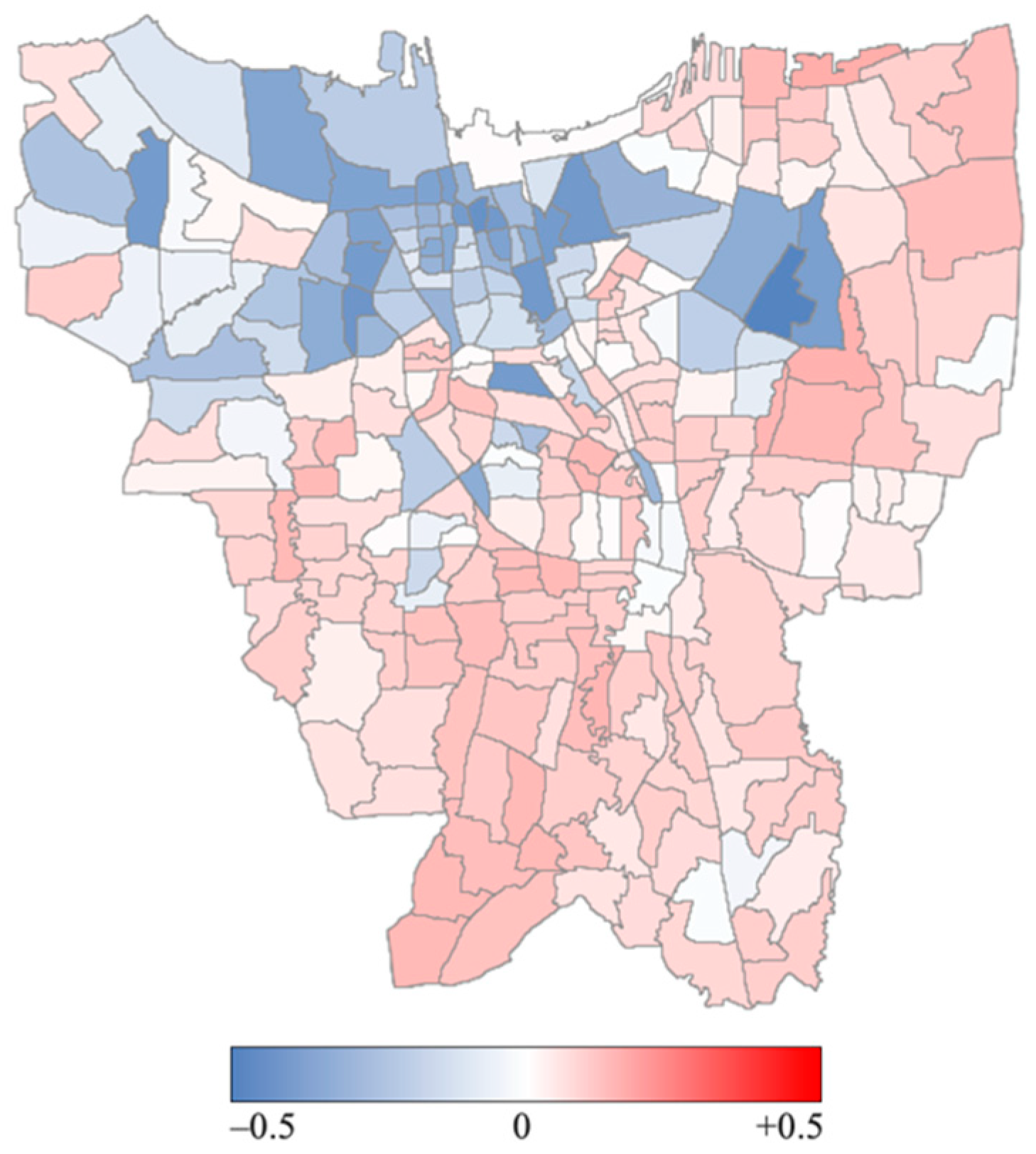
Figure 8 illustrates the distribution of the excess Simpson index value for each kelurahan in Jakarta. The excess Simpson index is the difference between the Simpson index value of that specific kelurahan and the Simpson index value of the whole Jakarta region. On average, the Simpson index value of all kelurahans was 0.645 (0.646), and the Simpson index value of the Jakarta region was 0.627 (0.628). Figure 8 shows a cluster of clear blue zones in the northwestern part of Jakarta. These blue zones indicate a lower level of diversity than the average diversity level of the entire Jakarta region. This visualized map is in line with the visualized maps of the inhabitants with Chinese and Javanese ethnicities, as shown in Figure 7a,b.
A question arises as to whether the analysis of religion as an additional characteristic adds value to the baseline ethnic composition. Ananta et al. [26] asserted that religion and language are two crucial inherent properties of ethnicity in Indonesia. However, a certain ethnicity is not necessarily exclusively associated with a certain religion. For instance, the Chinese appear to be primarily Buddhists and Confucians but have a significant Protestant and Catholic population of 43% (Table 3).

4.3. Agent-Based Model and Simulation

For simulation, we used NetLogo 6.3.0 [51], an open-source, agent-based modeling environment. We adopted the segregation model from Jan Lorenz (https://github.com/janlorenz/Schelling_on_GIS, accessed on 5 April 2022) and further modified this model to accommodate the purpose of the current study. Our model can be accessed on GitHub (http://github.com/hendro93/Segregation, accessed on 1 October 2022). We developed two separate simulation files: one file to investigate the impact of socioeconomic similarities and the other to investigate the impact of religious similarities. We upgraded the global parameter settings of housing constraints so that the experiment can be flexibly run. Moreover, we added six new monitoring panels using the BehaviorSpace feature of NetLogo, namely the excess average Simpson index, dissimilarity indexes for each ethnicity, and Moran’s I.
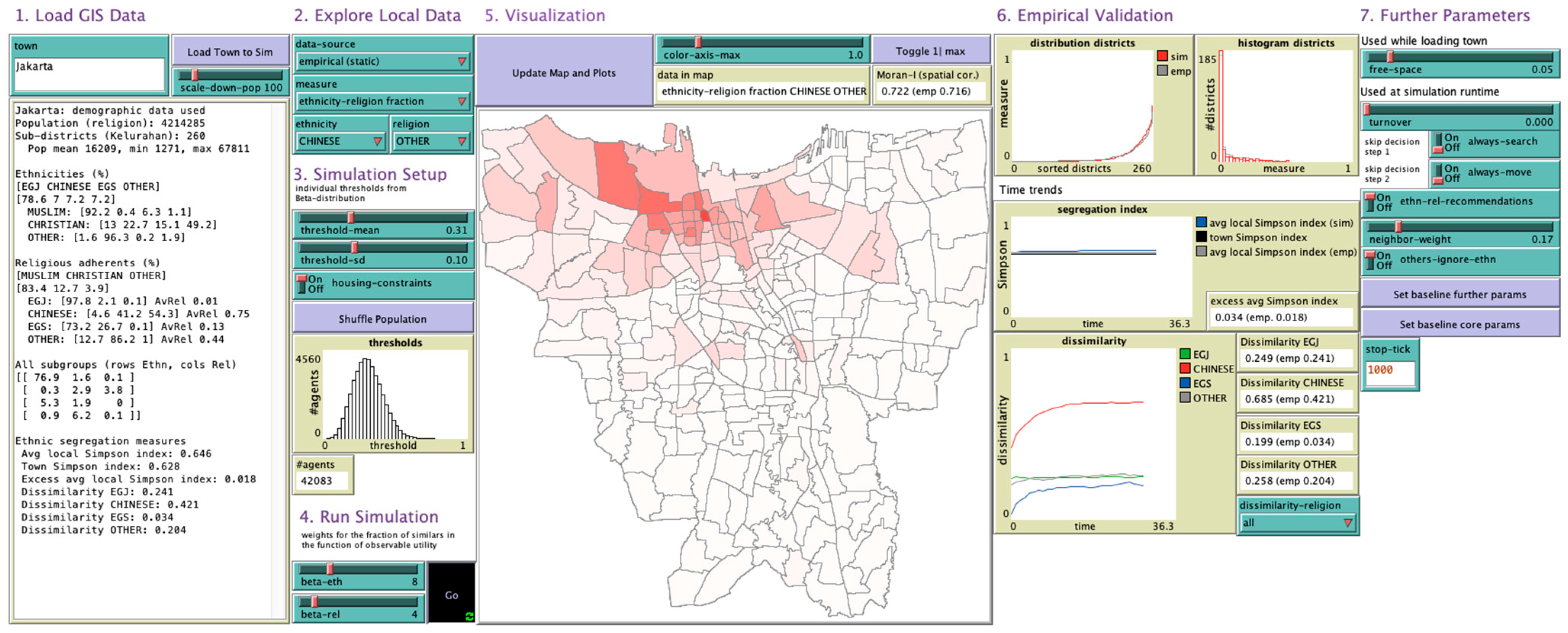
Figure 9 depicts the graphical user interface (GUI) of the simulation environment. The GUI consists of seven panels, i.e., load GIS data, explore local data, simulation setup, run simulation, visualization, empirical validation, and further parameters. The load GIS data panel is used to obtain a town’s GIS alongside the population quantity scaling, which will scale down the actual population quantity to a reasonable quantity of inhabitant agents. The explore local data panel consists of several features, including whether the map visualization is updated dynamically or only visualizes the final map when the simulation analysis ends. The “setup simulation” and “run simulation” panels enable users to set and monitor the agent’s utility function (Equation (1), i.e., threshold—mean, slider threshold—sd), housing constraints option, shuffle population button, Gumbel distribution plot, and a text box indicating the number of inhabitant agents in the simulation. The visualization panel enables adjustments to the parameters of the visualization maps. The empirical validation panel enables users to evaluate whether the values of the simulation output parameters (i.e., Simpson and dissimilarity indexes) are close to the actual values of the existing segregation condition. The “further parameters” panel is used to set numerous settings, i.e., the fraction of free space area within a region (i.e., free space), an agent’s incentive to relocate to another region (i.e., turnover), etc.
At the beginning of the simulation, we generated the inhabitant agents. For computational performance reasons, we scaled down the number of agents by a fraction of 100 of total Jakarta’s population. The actual total number of 4.2 million working inhabitants was thus scaled down to 42,000 agents. Each agent was assigned to one of the 260 kelurahan locations. On average, 162 agents inhabited each kelurahan. The number of agents we modeled stayed proportional to the ethnic composition in Jakarta.
Each agent in the model had the following properties: ethnicity (EGJ, CHINESE, EGS, or OTHER), socioeconomic status (LOW, MID, or HIGH), and religion (MUSLIM, CHRISTIAN, or OTHER). For each property, an agent had a threshold value that quantified the minimal fraction of the neighboring agents having similar properties for an agent to be satisfied with its current location.
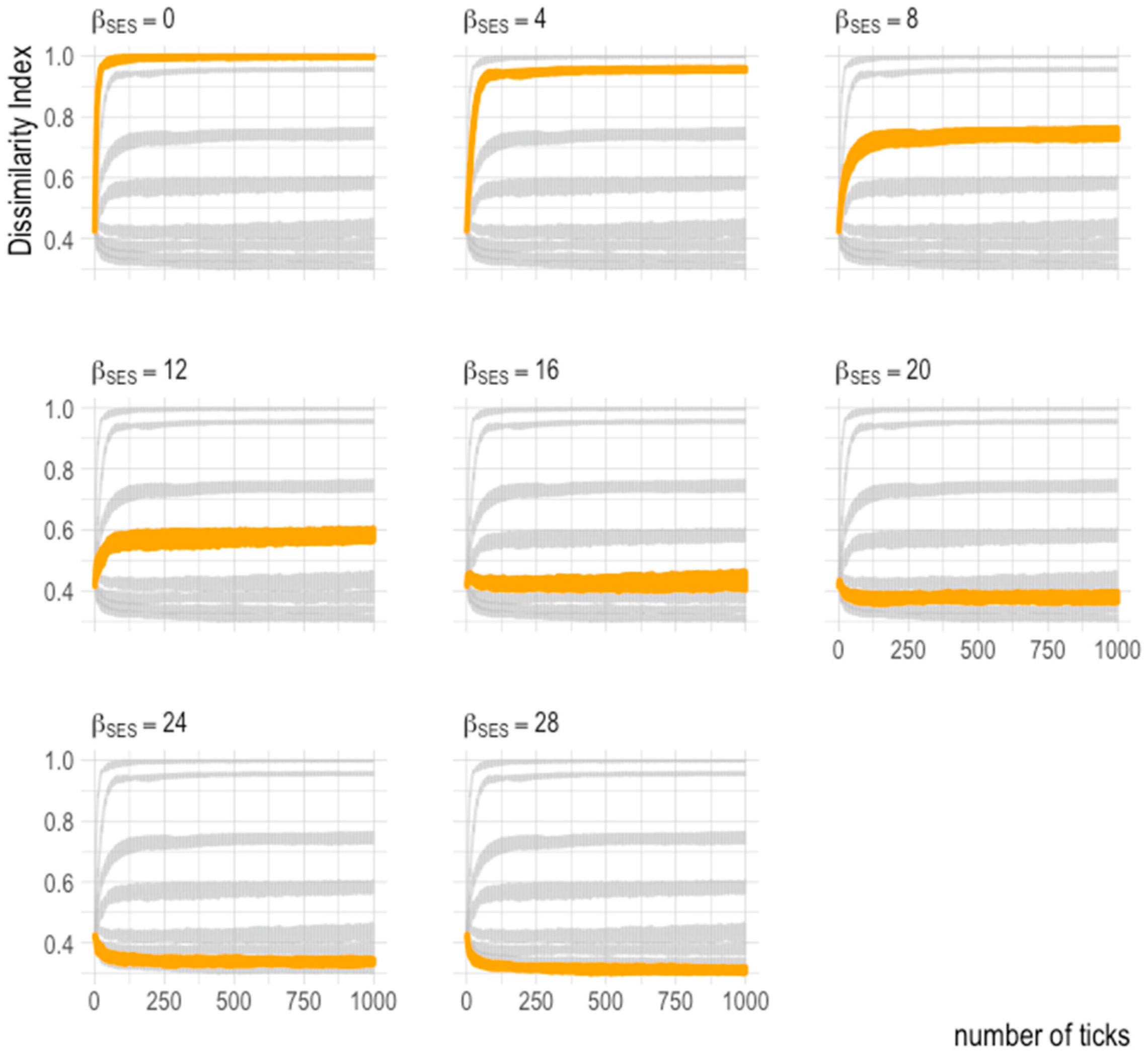
In line with the conceptual model, we executed two simulation scenarios to determine whether socioeconomic or religion is the most influential determinant of segregation. As shown in Table 4, in the first scenario, we increased the value of socioeconomic similarity β S E S incrementally (i.e., 0, 4, 8, 12, 16, 20, 24, 28). Likewise, in the second scenario (ethnicity–religion), we increased the value of religious similarity β r e l (i.e., 0, 4, 8, 12, 16, 20, 24, 28). We set each scenario’s “housing constraints” parameter to different values (i.e., on and off). We executed 10 simulation runs for each simulation setting using the BehaviorSpace feature of NetLogo. Each simulation setup was run for 1000 ticks (i.e., simulation time epoch). With 1000 ticks, each simulation reached a steady state (Appendix A). In reality, the simulation ran slowly due to the enormous number of agents (42,000 agents); therefore, it took an average of 11 h to complete each scenario. For each simulation setup, we recorded the value of six output parameters: the Simpson index, the dissimilarity index for each of the four ethnic groups, and the Moran index.

5. Results and Analysis

5.1. Socioeconomic Similarity and Segregation Pattern

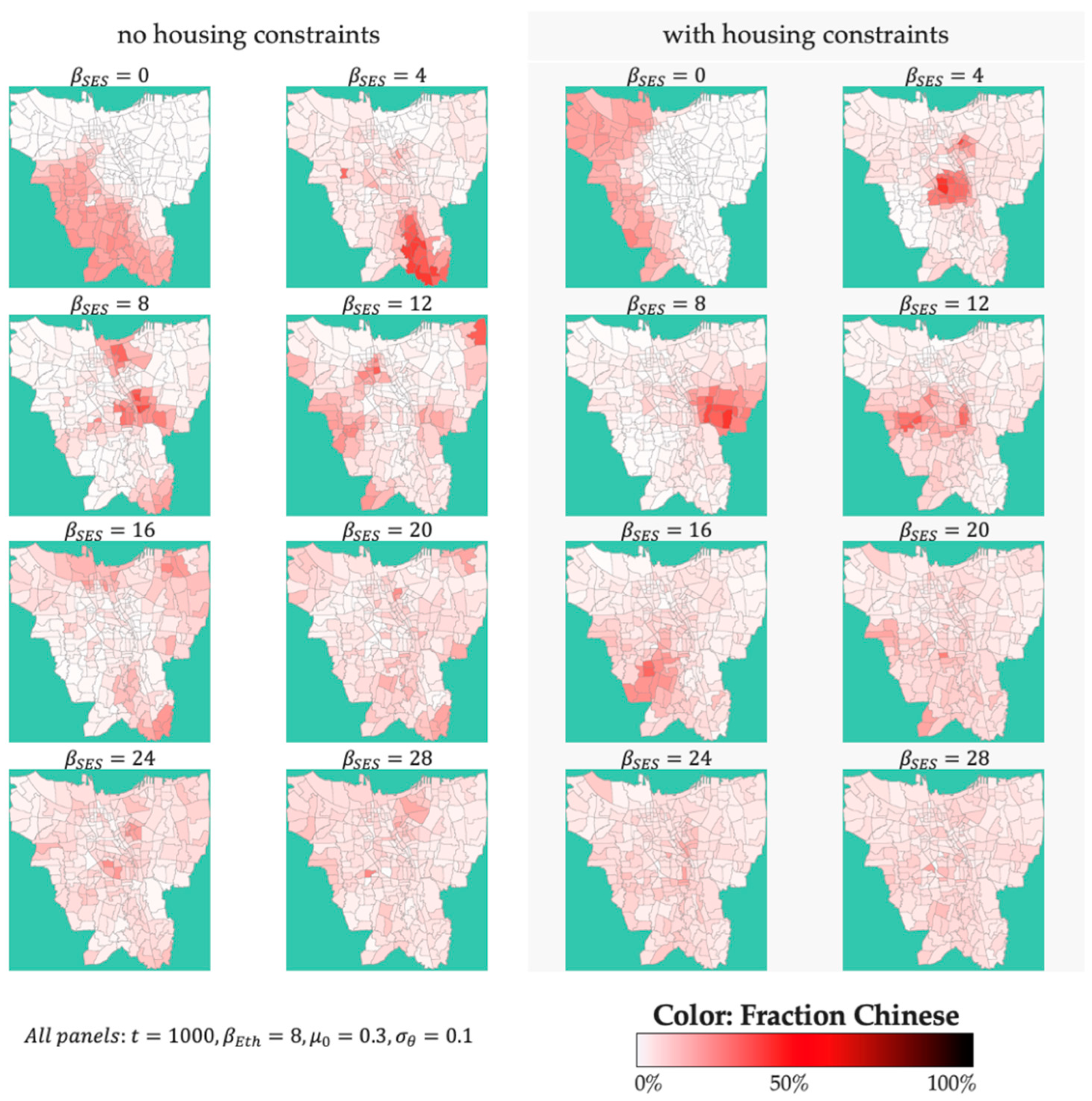
Figure 10 presents several plots indicating the impact of different levels of socioeconomic status β S E S   and housing constraints on the segregation pattern map. β S E S indicates the strength of the inhabitant agent’s preference for having neighbors with similar properties to the agent. The higher the β S E S , the less tolerance an agent has for accepting a neighbor having different socioeconomic status.
The simulated plots in which the inhabitants have no housing constraints preference reveal the cluster of population concentration increased as the β S E S   value increased from zero to four. However, as the β S E S increased, the concentration of people with similar properties decreased. A similar trend was also found in the simulation with active housing constraints preferences. The cluster of population concentration increased as the β S E S   value increased from zero to eight. However, as the β S E S   increased to a larger number, the concentration of people with similar properties decreased. The analysis of all the plots resulting from variation in the socioeconomic similarity values revealed that no single simulated plot had a similar pattern to the actual segregation pattern map used as the reference (Figure 7). Moreover, for a unique simulation setting, each simulation run led to a different segregation pattern. Thus, the segregation pattern was not consistent if we used the socioeconomic pattern variable as the dependent variable.
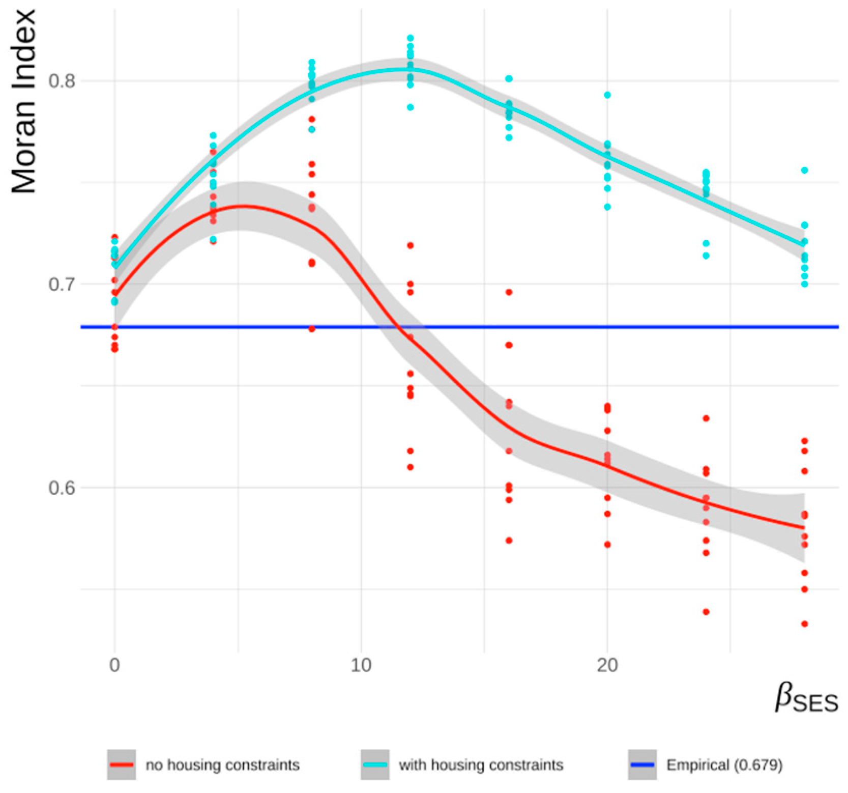
Figure 11 shows the simulated spatial autocorrelation index (i.e., Moran’s I) for each set of socioeconomic level β S E S in both scenarios with no housing constraints and with housing constraints. In agreement with the results shown in Figure 10, in the simulation condition of no housing constraints (i.e., red line), the value of Moran’s I increased with the increase in β S E S from 0 to 4. However, the Moran index drastically decreased as β S E S further increased from 8 to 28. For the simulation scenario with housing constraints (i.e., blue line), the Moran index value reached its peak (Moran’s I of 0.8) when the β S E S value of 12. Then, Moran’s I drastically decreases as β S E S further increased from 12 to 28. In general, the simulation runs with the housing constraints had higher spatial autocorrelation index (i.e., Moran’s I) than the ones with no housing constraints.

5.2. Religious Similarity and Segregation Pattern

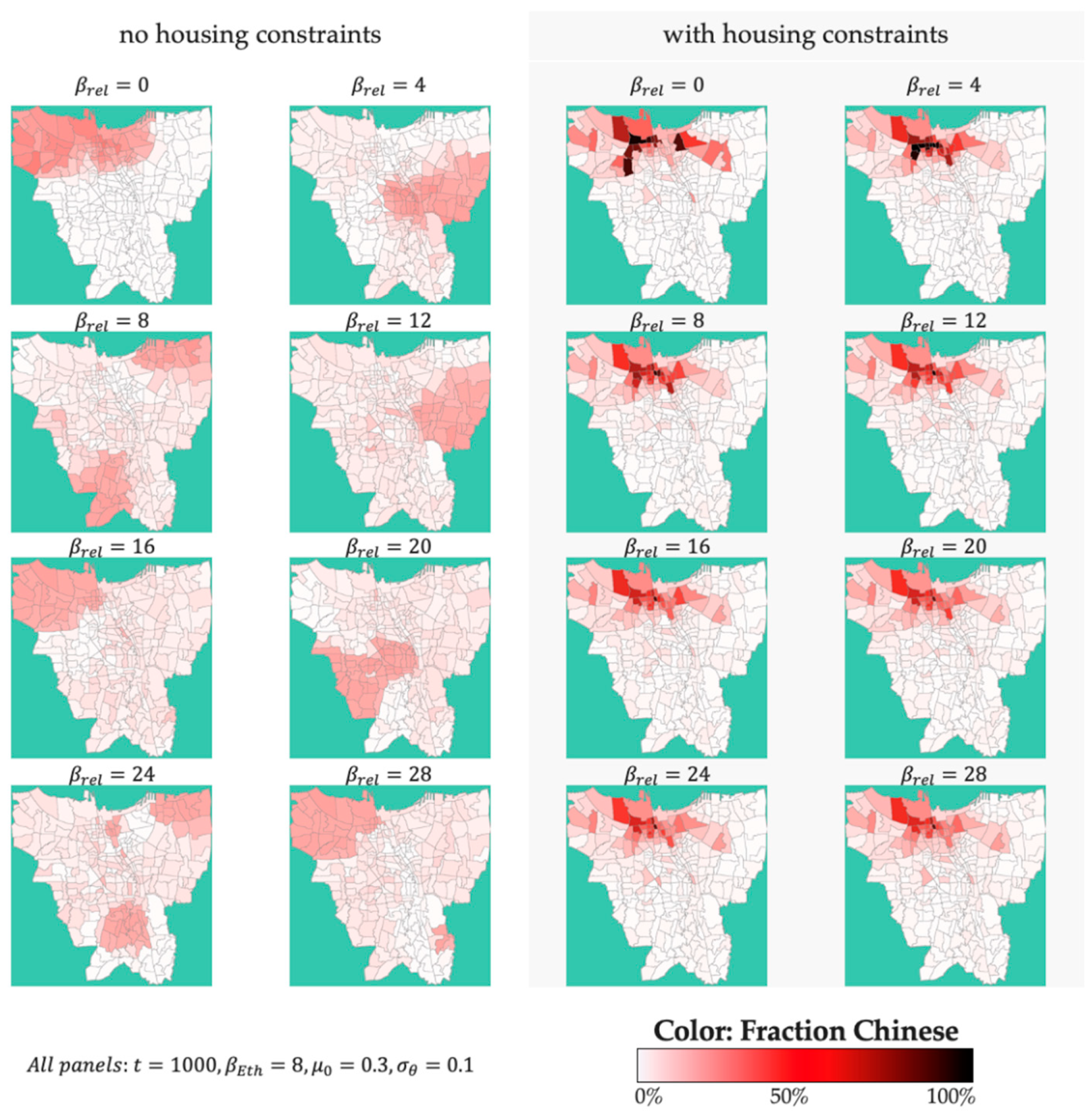
Figure 12 reveals several plots indicating the impact of the different levels of religious status similarity β R E L   and housing constraints on the segregation pattern. β R E L indicates the strength of the inhabitant agent’s preference for having a neighbor with similar religion to the agent. The higher the β R E L   , the less tolerance an agent has for accepting a neighbor having a different religion.
The plots for the scenario in which the inhabitants had no housing constraints preference revealed that the location of the clusters of population concentration constantly changed as the β r e l   value increased. In contrast, in plots from simulation scenarios where inhabitants had housing constraints preferences, the spatial pattern was more consistent. As can be seen, the cluster of population concentration was in the northwestern part of Jakarta. The simulated plots were consistent with the actual empirical condition (Figure 7), where people with Chinese ethnicity were concentrated in the northwestern part of Jakarta also.
Figure 13 shows that for the simulation runs in which the agents had no housing constraints (i.e., red line), the value of Moran’s I increased with the increase in β r e l from 0 to 12. However, the Moran index drastically decreased as β r e l further increased from 16 to 28. For simulation scenarios with housing constraints conditions (i.e., blue line), the Moran index value reached its peak (Moran’s I of 0.8) when we increased the β r e l value to eight. Then, the Moran index decreased as β r e l further increased to 12. Furthermore, the Moran index value became more constant as β r e l value increased from 12 to 28. The consistency between the spatial pattern maps derived from the simulation results and the actual empirical segregation data indicates that the impact of religion was more prominent than socioeconomic status in shaping the segregation patterns.
Figure 14 shows the relationship between religious preference β r e l   on the dissimilarity index of the inhabitants of Chinese ethnicity. The dissimilarity index is calculated using Equation (4). The blue line indicates the actual empirical value reference of 0.421. For the simulation runs with agents having housing constraints, the dissimilarity index reached a more constant value as the religious similarity β r e l increased beyond the value of 12. This finding is consistent with the results of the spatial autocorrelation index (Moran’s I), which indicated that the segregation cluster became more consistent as the value of the religious similarity β r e l became higher than 12.
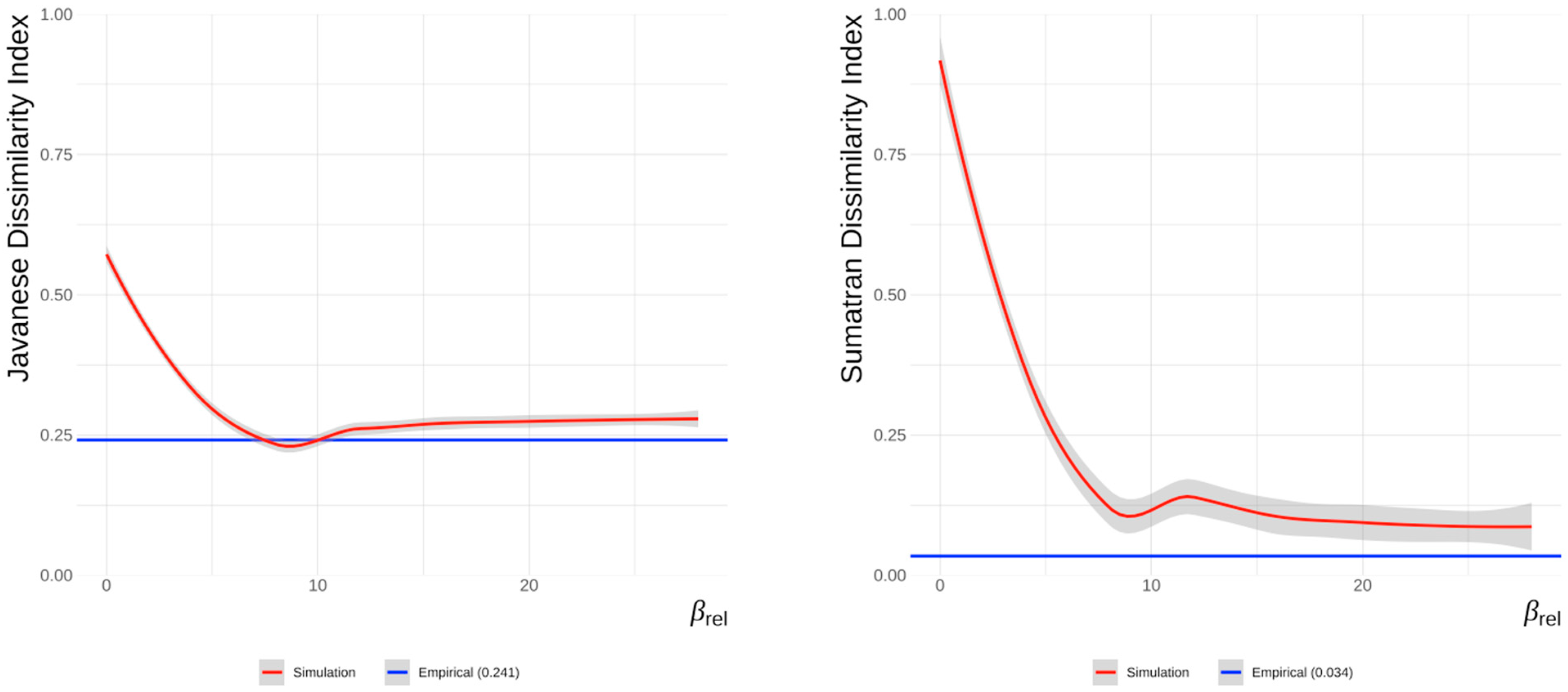
In addition to the analysis of the dissimilarity index for the inhabitants of Chinese ethnicity, we also analyzed the similarity index for the inhabitants of Javanese (i.e., EGJ) and Sumatran (i.e., EGS) ethnicities. As shown in Figure 15, the dissimilarity indexes for Javanese and Sumatran ethnicities reached their minimum value when β r e l equaled 8, and the dissimilarity indexes for Javanese and Sumatran ethnicities became constant values when β r e l reached the value of 12 and beyond. The dissimilarity index outputs derived from the simulation runs for Javanese and Sumatran ethnicities were closer to the empirical values than the dissimilarity indexes of the Chinese ethnicity (Figure 14). Moreover, the actual and empirical dissimilarity indexes for both Javanese (0.24) and Sumatrans (0.03) were lower than the dissimilarity index for the inhabitants of Chinese ethnicity (0.42).
Figure 16 shows the relationship between the population concentration value (i.e., the Simpson diversity index) and the inhabitants’ religious similarity β r e l . In line with our previous findings, the value of the excess Simpson diversity index also reached the minimum value when the religious similarity β r e l equaled 8 and stabilized when the religious similarity β r e l equaled 12 and beyond. The excess average Simpson index value was calculated by subtracting the city-level Simpson index value from the average kelurahan Simpson index.

6. Conclusions

In this study, we analyzed whether similarities in religion or socioeconomic status are more dominant in shaping segregation patterns in Jakarta. To do so, we extended Schelling’s segregation agent-based model by incorporating the random discrete utility formula to simulate the relocation decisions of the inhabitants. Utilizing actual census data from the 2010–2013 time period and the Jakarta GIS map, we simulated the migration of Jakarta inhabitants at the subdistrict level. We set the socioeconomic and religious similarities of the inhabitants as the independent variables and housing constraints as the moderating variable. As the dependent variables, we determined the inhabitants’ level of segregation (i.e., dissimilarity and Simpson indexes) and the residential segregation spatial patterns (i.e., Moran index and segregation maps). We concluded that religious similarities are more dominant than similarities in socioeconomic status in shaping residential segregation patterns in Jakarta.
Understanding the determining factors of residential segregation is valuable in regional development contexts. From this study, we gain a clear insight that religious similarity plays a more dominant role than socioeconomic similarity in shaping the residential segregation patterns of Jakarta. Thus, incorporating cultural considerations in planning and executing regional development programs is of high importance in a society where the religious aspect is dominant as it is in Jakarta. Abandoning the cultural aspect and applying a purely rational–economic approach in regional development decision-making may not bring a positive socioeconomic impact.
Studies on segregation mostly use descriptive and exploratory approaches in investigating clustering patterns derived from the inhabitants’ choice of residency. However, it is challenging for conventional research approaches to explore the inherent motives behind selecting a residential location, especially if the reasons of the residents are related to sensitive matters such as race, religion, etc. This study demonstrates the usefulness of spatial agent-based modeling and simulation to analyze the impact of an individual’s residential preference on residential segregation through the verification of its findings with the empirical demographic reality. Moreover, this study challenges the findings of previous studies concluding that the socioeconomic factor is the primary determinant of population segregation in Jakarta. On the contrary, this study confirms that similarities in religion are more dominant than similarities in socioeconomic status in shaping residential segregation patterns. Our simulation scenarios with religious housing constraints produced results very close to the actual empirical situation in terms of spatial segregation maps, dissimilarity index, and excess Simpson index value.

Author Contributions

Conceptualization, M.W.; methodology, H.K. and M.W.; software, H.K.; validation, H.K. and M.W.; formal analysis, H.K. and M.W.; data curation, H.K.; writing—original draft preparation, H.K.; writing—review and editing, H.K. and M.W.; visualization, H.K.; supervision, M.W.; funding acquisition, H.K. All authors have read and agreed to the published version of the manuscript.

Funding

This research received no external funding.

Data Availability Statement

Not applicable.

Conflicts of Interest

The authors declare no conflict of interest.

Appendix A

Figure A1. The Chinese socioeconomic dissimilarity index’s value β S E S reaches steady state after 1000 ticks (no housing constraints).
Systems 11 00020 g0a1
Figure A2. The Chinese socioeconomic dissimilarity index’s value β S E S reaches steady state after 1000 ticks (with housing constraints).
Systems 11 00020 g0a2
Figure A3. The Chinese religious dissimilarity index’s value β r e l   reaches steady state after 1000 ticks (no housing constraints).
Systems 11 00020 g0a3
Figure A4. The Chinese religious dissimilarity index’s value β r e l   reaches steady state after 1000 ticks (with housing constraints).
Systems 11 00020 g0a4
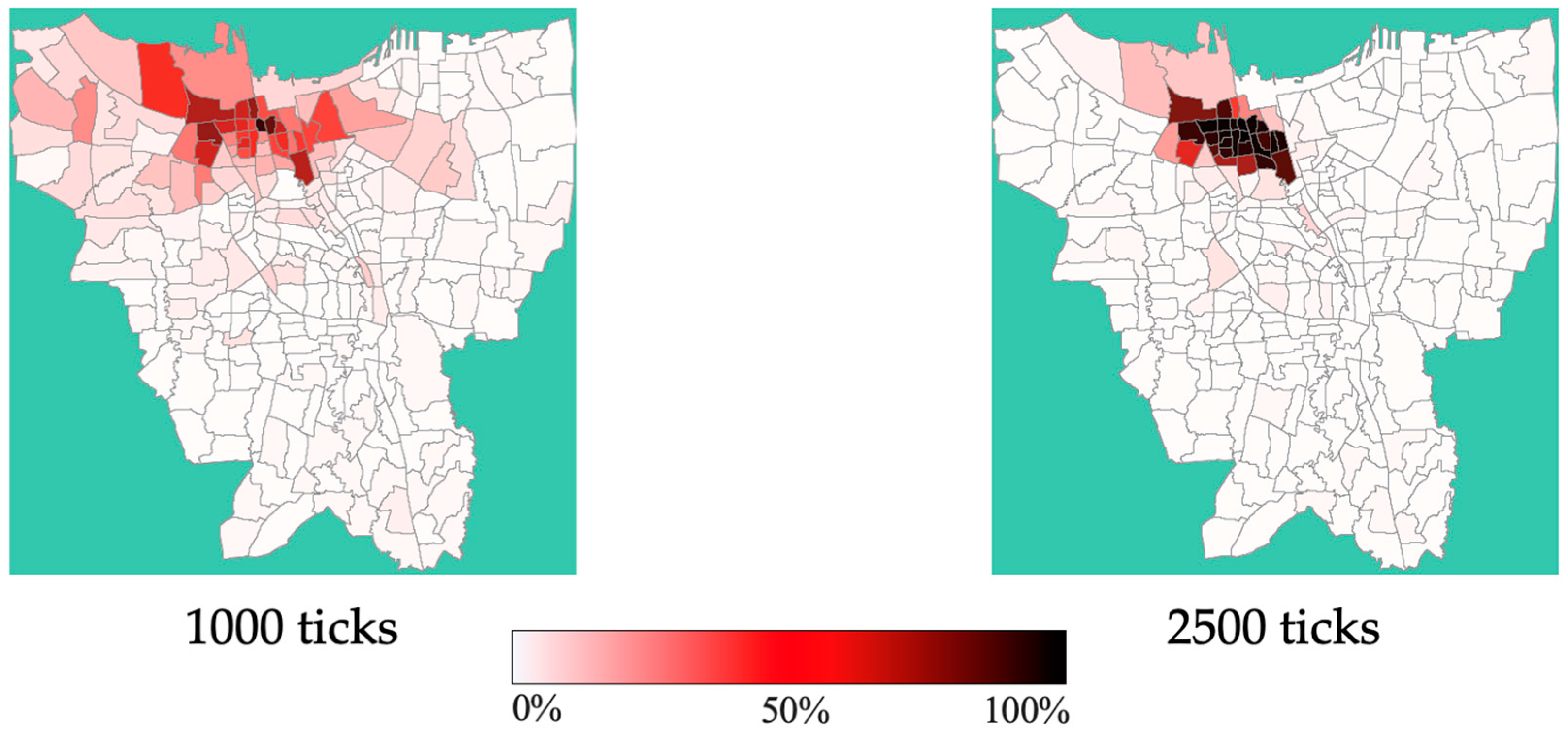
Figure A5. Spatial pattern results of the simulation with β E t h = 8 ,   β r e l = 8 ,   μ 0 = 0.3 ,   σ θ = 0.1 (with housing constraints).
Systems 11 00020 g0a5

Appendix B

Table A1. The design of the simulation experiments.
  Simulation ParameterValues
  Simulation replications10
  Simulation length1000 ticks
  GIS map (town)Jakarta
  Population scaling1:100 (i.e., 4,200,000 inhabitants Is projected to be 42,000 agents)
  Free-space fraction0.05
  Ethnicity focusCHINESE
  Housing constraints(false, true)
  Weight of ethnic similarity ( β e t h )8
  Weight of socioeconomic similarity ( β S E S )(0, 4, 8, 12, 16, 20, 24, 28)
  Weight of religious similarity ( β r e l )(0, 4, 8, 12, 16, 20, 24, 28)
  Town (GIS Data)Jakarta
  EthnicityEGJ, CHINESE, EGS, OTHER
  SESHIGH, MIDDLE, LOW
  ReligionMUSLIM, CHRISTIAN, OTHER
  Average threshold ( μ θ )0.3
  Heterogeneity threshold ( σ θ )0.1
  Color axis max0.1–5.0 (incremental 0.1)
  Turnover0
  Always searchfalse
  Always movefalse
  Ethnic-SES recommendationstrue
  Ethnic-Religion recommendationstrue
  Ignore “OTHER” Ethnictrue

Note

1
The Gumbel distribution is also known as generalized extreme value distribution type-I. It had a mean of 0.577 and a standard deviation of 1.283. In the decision to move, two random numbers were compared–one for each alternative. The difference in two Gumbel random variables had a logistic distribution with a mean of 0 and a standard deviation of 3.29.

References

  1. Yao, J.; Wong, D.W.; Bailey, N.; Minton, J. Spatial Segregation Measures: A Methodological Review. Tijdschr. Econ. Soc. Geogr. 2019, 110, 235–250. [Google Scholar] [CrossRef] [Green Version]
  2. Timberlake, J.M. Residential Segregation. In The Wiley Blackwell Encyclopedia of Race, Ethnicity, and Nationalism; John Wiley & Sons, Inc.: Hoboken, NJ, USA, 2015; pp. 1–4. [Google Scholar] [CrossRef]
  3. Lloyd, C.D.; Shuttleworth, I.G.; Wong, D.W.S. Social-Spatial Segregation: Concepts, Processes, and Outcomes, 1st ed.; Lloyd, C.D., Shuttleworth, I.G., Wong, D.W.S., Eds.; Bristol University Press: Bristol, UK, 2015. [Google Scholar] [CrossRef]
  4. Johnston, R.; Poulsen, M.; Forrest, J. Segregation Matters, Measurement Matters. Social-Spatial Segregation; Policy Press: Bristol, UK, 2014; pp. 13–44. [Google Scholar] [CrossRef]
  5. Nilsson, I.; Delmelle, E.C. On the link between rail transit and spatial income segregation. Appl. Geogr. 2020, 125, 102364. [Google Scholar] [CrossRef]
  6. Silver, D.; Byrne, U.; Adler, P. Venues and segregation: A revised Schelling model. PLoS ONE 2021, 16, e0242611. [Google Scholar] [CrossRef]
  7. Tomasiello, D.B.; Giannotti, M.; Feitosa, F.F. ACCESS: An agent-based model to explore job accessibility inequalities. Comput. Environ. Urban Syst. 2020, 81, 101462. [Google Scholar] [CrossRef]
  8. Caldwell, J.T.; Ford, C.L.; Wallace, S.P.; Wang, M.C.; Takahashi, L.M. Racial and ethnic residential segregation and access to health care in rural areas. Health Place 2017, 43, 104–112. [Google Scholar] [CrossRef] [PubMed] [Green Version]
  9. Benenson, I.; Hatna, E. Minority-Majority Relations in the Schelling Model of Residential Dynamics. Geogr. Anal. 2011, 43, 287–305. [Google Scholar] [CrossRef]
  10. Merino, S.M. Neighbors Like Me? Religious Affiliation and Neighborhood Racial Preferences among Non-Hispanic Whites. Religions 2011, 2, 165–183. [Google Scholar] [CrossRef]
  11. Tajima, Y.; Samphantharak, K.; Ostwald, K. Ethnic Segregation and Public Goods: Evidence from Indonesia. Am. Political Sci. Rev. 2018, 112, 637–653. [Google Scholar] [CrossRef]
  12. Zuccotti, C.v.; Lorenz, J.; Paolillo, R.; Sánchez, A.R.; Serka, S. Exploring the Dynamics of Neighbourhood Ethnic Segregation with Agent-Based Modelling: An Empirical Application to Bradford, UK. J. Ethn. Migr. Stud. 2022, 1–22. [Google Scholar]
  13. Browne, J. Segregation|History, Examples, & Facts|Britannica. 2020. Available online: https://bit.ly/3tffXHQ (accessed on 10 March 2022).
  14. Van Ham, M.; Tammaru, T.; de Vuijst, E.; Zwiers, M. Spatial Segregation and Socio-Economic Mobility in European Cities. SSRN Electron. J. 2021, 10277. [Google Scholar] [CrossRef]
  15. Prener, C.G. Demographic change, segregation, and the emergence of peripheral spaces in St. Louis, Missouri. Appl. Geogr. 2021, 133, 102472. [Google Scholar] [CrossRef]
  16. Zhang, T.; Duan, X.; Wong, D.W.; Lu, Y. Discovering income-economic segregation patterns: A residential-mobility embedding approach. Comput. Environ. Urban Syst. 2021, 90, 101709. [Google Scholar] [CrossRef]
  17. Florida, R.; Mellander, C. Technology, talent and economic segregation in cities. Appl. Geogr. 2020, 116, 102167. [Google Scholar] [CrossRef]
  18. Johnston, R.; Forrest, J.; Siciliano, F. Exploring the residential segregation of Chinese languages and language groups of the Indian subcontinent in Sydney. Geogr. Res. 2021, 59, 554–563. [Google Scholar] [CrossRef]
  19. Rademakers, R.; van Hoorn, A. Ethnic switching: Longitudinal evidence on prevalence, correlates, and implications for measuring ethnic segregation. J. Dev. Econ. 2021, 152, 102694. [Google Scholar] [CrossRef]
  20. Rukmana, D.; Ramadhani, D. Income Inequality and Socioeconomic Segregation in Jakarta; Urban Book Series; Springer International Publishing: Cham, Switzerland, 2021. [Google Scholar] [CrossRef]
  21. Xu, C.; Xiao, L.; Song, G.; Pan, B.; Liu, H. The impact of community residents’ occupational structure on the spatial distribution of different types of crimes. Habitat Int. 2021, 117, 102435. [Google Scholar] [CrossRef]
  22. Malanson, G.P.; Walsh, S.J. Agent-based models: Individuals interacting in space. Appl. Geogr. 2015, 56, 95–98. [Google Scholar] [CrossRef]
  23. Singh, V.K.; Gupta, A.K. Agent Based Models of Social Systems and Collective Intelligence. In Proceedings of the 2009 International Conference on Intelligent Agent and Multi-Agent Systems, IAMA, Chennai, India, 22–24 July 2009. [Google Scholar] [CrossRef]
  24. Schelling, T.C. Dynamic models of segregation†. J. Math. Sociol. 1971, 1, 143–186. [Google Scholar] [CrossRef]
  25. Hegselmann, R. Thomas, C. Schelling and James, M. Sakoda: The Intellectual, Technical, and Social History of a Model. J. Artif. Soc. Soc. Simul. 2017, 20, 15. [Google Scholar] [CrossRef]
  26. Ananta, A.; Nurvidya Arifin, E.; Sairi Hasbullah, M. Demography of Indonesia’s Ethnicity; ISEAS Publishing: Singapore, 2018. [Google Scholar] [CrossRef]
  27. Firman, T. New town development in Jakarta Metropolitan Region: A perspective of spatial segregation. Habitat Int. 2004, 28, 349–368. [Google Scholar] [CrossRef]
  28. Stepinski, T.F.; Dmowska, A. Imperfect melting pot—Analysis of changes in diversity and segregation of US urban census tracts in the period of 1990–2010. Comput. Environ. Urban Syst. 2019, 76, 101–109. [Google Scholar] [CrossRef] [Green Version]
  29. Johnston, R.; Poulsen, M. The Geography of Ethnic Residential Segregation: Of Five Countries a Comparative Study. Ann. Assoc. Am. Geogr. 2013, 97, 713–738. [Google Scholar] [CrossRef] [Green Version]
  30. Poston, D.L.P., Jr.; Compton, D.R.; Xiong, Q.; Knox, E.A. The Residential Segregation of Same-Sex Households from Different-Sex Households in Metropolitan USA, circa-2010. Popul. Rev. 2017, 56, 1–29. [Google Scholar] [CrossRef]
  31. Sabater, A.; Catney, G. Unpacking Summary Measures of Ethnic Residential Segregation Using an Age Group and Age Cohort Perspective. Eur. J. Popul. 2019, 35, 161–189. [Google Scholar] [CrossRef] [PubMed] [Green Version]
  32. Fong, E.; Chan, E. Residential Patterns among Religious Groups in Canadian Cities. City Community 2011, 10, 393–413. [Google Scholar] [CrossRef]
  33. Roy, D.; Lees, M. Understanding resilience in slums using an agent-based model. Comput. Environ. Urban Syst. 2020, 80, 101458. [Google Scholar] [CrossRef]
  34. Zwiers, M.; van Ham, M.; Manley, D. Trajectories of ethnic neighbourhood change: Spatial patterns of increasing ethnic diversity. Popul. Space Place 2018, 24, e2094. [Google Scholar] [CrossRef] [Green Version]
  35. Zuccotti, C.V. Changes in Ethnic Spatial Segregation across English Housing Market Areas (2001–2011): Identifying Ethnic and Context Configurations. Investig. Geogr. 2021, 2021, 101–120. [Google Scholar] [CrossRef]
  36. Stroub, K.J.; Richards, M.P. From Resegregation to Reintegration: Trends in the Racial/Ethnic Segregation of Metropolitan Public Schools, 1993–2009. Am. Educ. Res. J. 2013, 50, 497–531. [Google Scholar] [CrossRef]
  37. Hu, L.; Moayyed, H.; Frank, N. Racial/ethnic and class segregation at workplace and residence: A Los Angeles case study. J. Urban Aff. 2020, 44, 907–925. [Google Scholar] [CrossRef]
  38. Catney, G. The complex geographies of ethnic residential segregation: Using spatial and local measures to explore scale-dependency and spatial relationships. Trans. Inst. Br. Geogr. 2018, 43, 137–152. [Google Scholar] [CrossRef] [Green Version]
  39. Ardestani, B.M.; O’Sullivan, D.; Davis, P. A multi-scaled agent-based model of residential segregation applied to a real metropolitan area. Comput. Environ. Urban Syst. 2018, 69, 1–16. [Google Scholar] [CrossRef]
  40. Sage, L.; Flache, A. Can Ethnic Tolerance Curb Self-Reinforcing School Segregation? A Theoretical Agent Based Model. J. Artif. Soc. Soc. Simul. 2021, 24, 4544. [Google Scholar] [CrossRef]
  41. Loughran, T.; Fieldhouse, E.; Lessard-Phillips, L.; Bentley, L. Disruptive Norms: Assessing the Impact of Ethnic Minority Immigration on Nonimmigrant Voter Turnout Using a Complex Model. Soc. Sci. Comput. Rev. 2020, 38, 422–442. [Google Scholar] [CrossRef] [Green Version]
  42. Ta, N.; Kwan, M.-P.; Lin, S.; Zhu, Q. The activity space-based segregation of migrants in suburban Shanghai. Appl. Geogr. 2021, 133, 102499. [Google Scholar] [CrossRef]
  43. Badan Pusat Statistik. Hasil Sensus Penduduk 2020. Ber. Resmi Stat. 2021, XVI, 1–16. [Google Scholar]
  44. Association American Psychological. Education and Socioeconomic Status Factsheet. America Psychological Association. 2015. Available online: https://www.apa.org/pi/ses/resources/publications/education (accessed on 5 April 2022).
  45. Bruch, E.E.; Mare, R.D. Preferences and Pathways to Segregation: Reply to Van de Rijt, Siegel, and Macy. Am. J. Sociol. 2009, 114, 1181–1198. [Google Scholar] [CrossRef] [PubMed] [Green Version]
  46. Manski, C.F. The structure of random utility models. Theory Decis. 1977, 8, 229–254. [Google Scholar] [CrossRef]
  47. Massey, D.S.; Denton, N.A. The Dimensions of Residential Segregation. Soc. Forces 1988, 67, 281–315. [Google Scholar] [CrossRef]
  48. Kelly, A. A new composite measure of ethnic diversity: Investigating the controversy over minority ethnic recruitment at Oxford and Cambridge universities. Br. Educ. Res. J. 2019, 45, 41–82. [Google Scholar] [CrossRef]
  49. Glen, S. Moran’s I: Definition, Examples—Statistics How To. 2016. Available online: https://www.statisticshowto.com/morans-i/ (accessed on 5 April 2022).
  50. Ukrainski, P. How Are Objects’ Quantitative Characteristics Spatially Distributed? Finding an Answer with Global Moran’s I. 2018. Available online: http://www.50northspatial.org/global-morans-i-spatial-autocorrelation/ (accessed on 10 March 2022).
  51. Wilensky, U. NetLogo. Center for Connected Learning and Computer-Based Modeling, Northwestern University, Evanston, IL. 1999. Available online: https://ccl.northwestern.edu/netlogo/ (accessed on 10 March 2022).
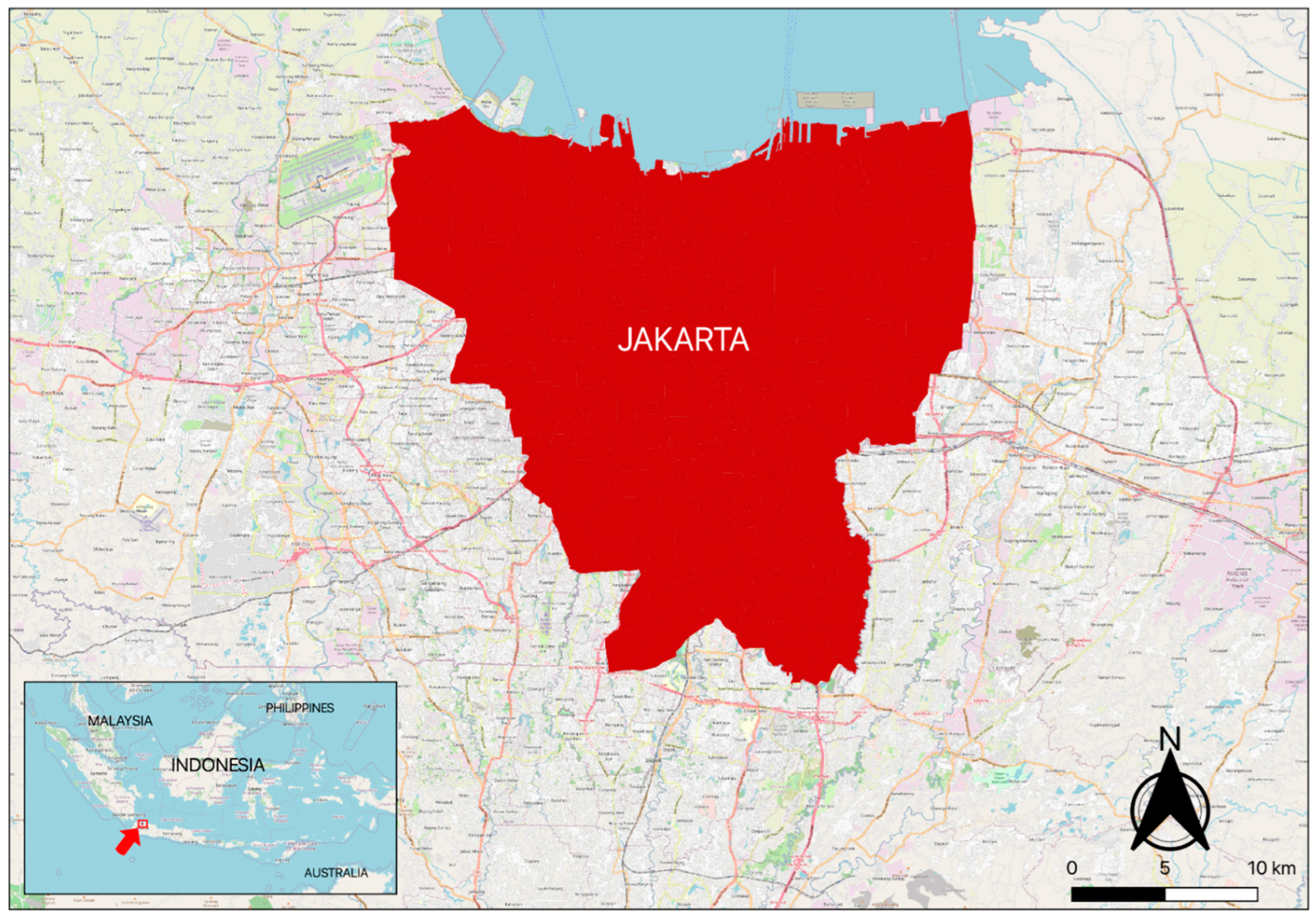
Figure 1. Map of Jakarta (The map’s inset shows the position of Jakarta in Indonesia).
Systems 11 00020 g001
Figure 2. The distribution of Jakarta’s population.
Systems 11 00020 g002
Figure 3. Spatial pattern of Jakarta’s population based on religious similarities.
Systems 11 00020 g003
Figure 4. Spatial pattern of Jakarta’s population based on socioeconomic status.
Systems 11 00020 g004
Figure 5. The conceptual research model.
Systems 11 00020 g005
Figure 6. The logic of an inhabitant agent.
Systems 11 00020 g006
Figure 7. Distribution of ethnic groups in Jakarta: (a) Javanese, (b) Chinese, (c) Sumatran, and (d) Other.
Systems 11 00020 g007
Figure 8. Distribution of excess local Simpson index value in Jakarta.
Systems 11 00020 g008
Figure 9. The graphical user interface of the agent-based simulation.
Systems 11 00020 g009
Figure 10. The impact of socioeconomic similarity and housing constraints on the segregation pattern.
Systems 11 00020 g010
Figure 11. The influence of socioeconomic similarity ( β S E S ) on Moran index.
Systems 11 00020 g011
Figure 12. The impact of religious similarity and housing constraints on the segregation pattern.
Systems 11 00020 g012
Figure 13. The influence of religious similarity ( β r e l ) on Moran index.
Systems 11 00020 g013
Figure 14. The relationship between β r e l and Chinese dissimilarity index (with housing constraints).
Systems 11 00020 g014
Figure 15. The relationship between β r e l and Javanese and Sumatran dissimilarity indexes (with housing constraints).
Systems 11 00020 g015
Figure 16. Excess average Simpson index on β r e l with housing constraints (ethnicity and religion interaction).
Systems 11 00020 g016
Table 1. The position of this study.
No.StudyMethod(s)Preference(s)Location(s)Finding
Statistical AnalysisSpatial AnalysisABMEthnic/RaceReligionSocioeconomic Status
1Florida and Mellander [17] The U.S. (country level)Technology and talent are typically associated with higher levels of economic segregation but not with increased economic segregation growth over time.
2Johnston et al. [18] Sydney, Australia (city level)There is consistent evidence of a significant degree of segregation among those speaking 17 languages at the neighborhood level.
3Loughran et al. [41] The U.K. (country level)An increase in the immigration rate causes a small but significant increase in voter turnout among the nonimmigrant population. Higher levels of civil obligation among immigrants lead to higher turnout rates among nonimmigrants over time.
4Nilsson and Delmelle [5] The U.S. (country level)There is no statistical evidence that rail transport investment spurred changes in neighborhood income diversity. Similarly, no significant impact of new or expanded rail transit lines on metropolitan-wide income segregation.
5Prener [15] St. Louis, Missouri (U.S.) (city level)St. Louis’s peripheral areas expanded over the twentieth century, first in the city and then in the county, creating dual zones of exploitation where poverty, segregation, and income inequality remain persistent.
6Rademakers and van Hoorn [19] Indonesia, the U.S., and India (country level)Ethnic switching is accurate and highly relevant for studying ethnic diversity and segregation.
7Rukmana and Ramadhani [20] Jakarta Metropolitan Area (inter-provincial level)The correlation among income inequality, socioeconomic segregation, and other institutional and contextual factors caused residential Segregation in Jakarta.
8Tomasiello et al. [7] Sao Paulo, Brazil (city level)ACCESS allowed the residential location of different social status groups to be depicted with a high correlation to the observed situation.
9van Ham et al. [14] Metropolitan regions across Europe (city level)Socioeconomic segregation is the outcome of a combination of inequality, poverty, and the spatial organization of urban housing markets.
10Xu et al. [21] 2055 communities in City ZG, a megacity along the southern coast of China (subdistrict level)Different occupational groups have different social characteristics and socioeconomic status, and so do their different impacts on various criminal activities.
11Zhang et al. [16] Shenzhen, China (city level)The more segregated communities, which are composed of the poorest and richest groups, are mostly in the peripheral regions of the city, while the inner city has lower levels of segregation due to transit of accessibility differences.
12This studyJakarta (provincial level)Inhabitants’ religious similarity is more dominant than socioeconomic status similarity in shaping residential segregation patterns.
Table 2. The religion correlation matrix of Jakarta inhabitants.
AttributesIslamProtestantCatholicHinduBuddhaConfucianOthers
Islam10.5020.2260.1970.1060.2030.013
Protestant0.50210.7990.3470.6160.481−0.071
Catholic0.2260.79910.3710.5490.502−0.141
Hindu0.1970.3470.37110.0910.1890.143
Buddha0.1060.6160.5490.09110.489−0.080
Confucian0.2030.4810.5020.1890.4891−0.133
Others0.013−0.071−0.1410.143−0.080−0.1331
Table 3. The religious composition of an ethnic group in Jakarta [26].
EthnicReligion (%)
IslamProtestantCatholicBuddhistConfucianHinduOther
(Christianity)(Other)
Javanese97.171.590.970.10-0.160.01
Betawi97.101.600.600.60--0.10
Sundanese99.400.500.10
Chinese5.0025.0018.0049.003.00
Batak44.0055.00---1.00
Minangkabau100.00------
Malay98.770.980.25
Table 4. The design of the simulation experiments.
  Simulation ParameterValues
  Simulation replications10
  Simulation length1000 ticks
  GIS map (town)Jakarta
  Population scaling1:100 (i.e., 4,200,000 inhabitants Is projected to be 42,000 agents)
  Free-space fraction0.05
  Ethnicity focusCHINESE
  Housing constraints(false, true)
  Weight of ethnic similarity ( β e t h )8
  Weight of socioeconomic similarity ( β S E S )(0, 4, 8, 12, 16, 20, 24, 28)
  Weight of religious similarity ( β r e l )(0, 4, 8, 12, 16, 20, 24, 28)
  Other parametersThe simulation detail is listed in Appendix B,
Disclaimer/Publisher’s Note: The statements, opinions and data contained in all publications are solely those of the individual author(s) and contributor(s) and not of MDPI and/or the editor(s). MDPI and/or the editor(s) disclaim responsibility for any injury to people or property resulting from any ideas, methods, instructions or products referred to in the content.