The Decision-Making for the Optimization of Finance Lease with Facilities’ Two-Dimensional Deterioration

Abstract

In the past, most companies in developing countries usually own facilities or equipment for running their businesses. However, for some managerial and financial reasons, the situation may change. Recently, leasing facilities is becoming more popular than purchasing them. Furthermore, since the deterioration of equipment or facilities depends on both time and usage, when considering only one of the two factors, the deterioration estimation for the leased facilities could be distorted. Therefore, in such cases, a two-dimensional failure model would be appropriate for dealing with such problems. In this study, in order to determine the optimal lease decision for lessors, we use analytical models and efficient solution algorithms based on the two deterioration factors (time and usage). However, such complex mathematical models are difficult to apply in real cases, and therefore the study proposes the design of computerized system architecture and the corresponding solution algorithms to enhance the practicality of the applications. Besides, a nonhomogeneous Poisson process is employed to describe the successive failure times of the leased facility. Finally, the application and sensitivity analyses will provide managerial implications and suggestions for decision-makers under different preventive maintenance alternatives.

1. Introduction

In the last two decades, the majority of companies preferred to purchase their own equipment and facilities to run their business. It is possible, however, that the situation may change due to some managerial and financial reasons. Accordingly, there are more and more companies choosing to lease equipment and facilities instead of buying them outright. In the manufacturing industry, Pongpech and Murthy [1] gave two reasons why leasing facilities will become more popular: (1) Rapid technical advancements cause technological obsolescence, with newer and better equipment arriving on the market at a quicker rate. (2) The cost of owning facilities is getting too expensive. In addition, the financial benefit is one of the primary reasons that influence the decision of companies to lease facilities instead of buying them. As a result of leasing, companies are able to better match their cash flow with revenue by making better use of their facilities. In other words, a leasing policy is a good way to reduce companies’ tax obligations and avoid the risk of investing in new facilities. Accordingly, numerous studies began focusing on finance leases in different equipment, facilities, or machines. Nisbet and Ward [2] investigated the leasing of radiation equipment for medical facilities and hospitals and provided an indication between purchase and lease in terms of cost consideration. Optimal pricing rules for remanufacturing leased items were presented by Aras et al. [3]. Bourjade et al. [4] investigated the influence of aircraft leasing on financial performance and stability.

However, leasing facilities or equipment create new challenges for both the lessor and the lessee. The lessor may be required to offer preventive maintenance services and a free repair warranty to its lessee for the duration of the lease. When the lessor prepares the lease contract for the lessee, the costs may be considered. In general, most contracts will stipulate penalties for repeated failures, unfulfilled maintenance service and repair not conducted within an acceptable time limit, and so on ([5,6,7]). In other words, leasing facilities are frequently combined with preventive maintenance and free repair service that the lessor provides to the lessee as part of a contract. Iskandar and Husniah [8] proposed an imperfect preventive maintenance policy to reduce lease equipment’s failure rate. In this lease contract, the lessor has to pay the related costs of preventive maintenance, repair, and penalty for his customers. Zhang et al. [9] expressed their viewpoint on the leasing facilities problem. In their perspective, in order to avoid the burden of purchasing facilities in the short term, most companies might choose to lease them rather than buy them. The lessor should, however, provide equipment maintenance services to lessees in order to increase their lease intention for the purpose of expanding their market share. Thus, most lease contracts include maintenance services in order to attract lessors. Liu et al. [10] proposed a non-cooperative game model to discuss the issue of preventive maintenance service of leased equipment between lessors and lessees. They considered that a cost-sharing contract can be designed to achieve the maximum revenue as in a cooperative game between lessors and lessees. According to the above-mentioned, they reasoned that most lessees or companies would lease rather than buy to avoid the expense of acquiring facilities. Lessors should, however, continue to meet lessees’ demands for facilities maintenance in order to enhance lease intention and gain market share. As a result, it is common for most leasing contracts to include preventive maintenance services in order to attract lessees.

Typically, since the lessor wants to attract customers to accept the capital or financial lease contract, he/her might provide a warranty with preventive maintenance service to customers. Accordingly, periodic and sequential preventive maintenance policies are often applied in lease contracts in practice. A periodic preventive maintenance policy is the manufacturer providing its maintenance work with equal time intervals. Sequential preventive maintenance policy is different from the periodic preventive maintenance policy. This policy is characterized by the search for the optimal number of maintenance actions to be performed during a given period and the optimal intervals between two maintenance activities. Therefore, the policy is to fulfill the system degeneration process because a system is maintained at an unequal sequence of intervals. Park et al. [11] proposed a model for calculating the ideal duration and number of preventive maintenances based on minimum repairs after breakdowns. Yeh and Lo [12] demonstrated that the ideal interval between two consecutive preventive maintenance activities is equal to the degree of maintenance. They also proved their model with an equivalent degree of preventive maintenance is the best method to decrease the related costs. Jung and Park [13] developed a periodic preventive maintenance policy to obtain the optimal number and the optimal period for warranty service by minimizing the long-run maintenance costs. Seo and Bai [14] proposed a periodic preventive maintenance strategy for two scenarios where the maintenance time might be disregarded or not. Yeh and Chang [15] determined the best failure rate and periodic maintenance strategy in a lease duration. Hu and Zong [16] relaxed some constraints under which the lease period is proposed in Pongpech and Murthy’s [1] model, and established the best lease duration and preventive maintenance method to minimize total cost per unit time. Das and Sarmah [17] provided an overview of optimization methods for maintenance and replacement in heavy-process industries. Yeh et al. [5] evaluated the effects of various maintenance cost functions on a leased product with a Weibull lifetime distribution and periodic maintenance policy. Chang and Lo [18] evaluated the impact of lease terms on maintenance strategy for leased equipment with residual value. Bouguerra et al. [19] created a mathematical model for various maintenance alternatives when customers choose to purchase an extended warranty. They discovered a viable compromise to establish a win-win situation between producers and customers in terms of warranty costs. Chang and Lin [20] developed an ideal maintenance policy for repairable items with extended warranties. They discovered that manufacturers should give a slight discount to consumers who have purchased extended warranty contracts in order to increase earnings. Kim and Ozturkoglu [21] transformed the traditional preventive maintenance problem into an integer programming problem. Shafiee et al. [22] create a mathematical model to simultaneously calculate the ideal burn-in time, optimal number of maintenance operations, and appropriate maintenance degree. Shafiee’s model’s primary contribution is that it measures the consequences of maintenance action when the failure rate is constant. Khojandi et al. [23] investigated the optimal lifetime-reward maintenance strategies for perfect and imperfect maintenance situations. They showed the tradeoff between the virtual age of the systems and the incentive rate for decision-makers. Yuan and Lu [24] suggested an effective way to solve a reliability-based optimization issue that combines the weighted approach with sequential preventive maintenance optimization. Lu et al. [25] proposed a joint model of sequential preventive maintenance and quality improvement for deteriorating manufacturing systems. The study is more appropriate for maintaining machines in a production system. Wang and Djurdjanovic [26] also proposed a joint model for preventive maintenance scheduling with consideration of inventory and transportation management. They seek an integrated decision-making policy to trigger preventive maintenance for working parts. Zhou et al. [27] proposed a sequential preventive maintenance model with a reducing failure factor. The model was applied to urban bus systems’ maintenance works. García and Salgado [28] discussed a case study to analyze the selection of preventive maintenance strategies in multistage industrial equipment. Their study utilized some individual indicators to evaluate which preventive maintenance strategies are better. Alrifaey et al. [29] designed a hybrid reliability-centered maintenance model to optimize the preventive maintenance work for an electrical gas turbine generator. Since the preventive maintenance work involves the scheduling issue, they utilized a particle swarm optimization algorithm to obtain the optimal solution. Tsarouhas [30] applied preventive maintenance models based on an NHPP assumption to the ice cream industry. Tsarouhas used RAM (Reliability, Availability, and Maintainability) analytical methods for monitoring a firm’s machine status of manufacturing systems. Lastra et al. [31] proposed the applicability of additive manuring processes to improve the works of preventive maintenance. They considered that the spare parts would play an important role in machine maintenance. Diatte et al. [32] proposed a methodology for improving an automobile brake system, and the methodology makes the integration of the equipment’s reliability, availability, and maintainability into system engineering and dependability analyses for reducing related costs and increasing a system’s reliability.

Since the degradation of industrial equipment or facilities is affected not only by time but also by usage, just considering one of them may skew the assessment of equipment deterioration. As a result, a two-dimensional failure model would be appropriate for dealing with such issues. Baik et al. [33] addressed two-dimensional failure modeling for a system that is degrading owing to two factors: age and usage. In their study, the two-dimensional situation was applied to the concept of minimal repair, and the failures were characterized using the Bivariate Weibull model. He et al. [34] utilized a similar concept in order to assess the reliability of piezoelectric micro-actuators by taking two factors into account: the driving voltage and the temperature of the actuator. As a means of solving a two-dimensional warranty problem, Murthy et al. [35] used Beta-Stacy and Bivariate Pareto distributions. In order to estimate the expected cost under a free-replacement warranty, Kim and Rao [36] used a bivariate exponential distribution. Pal and Murthy [37] also utilized a Bivariate Exponential distribution to estimate machinery’s repair cost. It offered manufacturers with guidance on how to offer two-dimensional maintenance service to customers with appropriate duration. Shahanaghi et al. [38] designed a two-dimensional extended warranty contract for automobile manufacturers. They focused on how to improve preventive maintenance plans based on the length and usage of the warranty. Huang et al. [39] used a bivariate Weibull distribution to analyze the repair costs with periodic preventive maintenance. Huang et al. [40] designed a customized warranty with two-dimensional deterioration for different usage style customers. Their study result indicated that the customized warranty policy is beneficial by providing an effective mechanism to decrease the related costs. Park et al. [41] proposed a warranty policy with consideration of two-dimensional deterioration especially focusing on the post-warranty period. Dong et al. [42] proposed an opportunistic maintenance strategy for improving system availability and reducing warranty costs. In their model, a two-dimensional warranty was taken into consideration, and a designed reliability threshold is used to ensure the utilization is above a certain level. Wang et al. [43] proposed and applied punctual and unpunctual preventive maintenance policies with two-dimensional deterioration in automobile industries. Dong et al. [44] studied a multi-component system with two-dimensional deterioration. In order to solve their proposed model efficiently, they utilized beetle antennae search with particle swarm optimization to achieve the objectives of lower cost and higher system availability.

According to the discussions above, the study takes a two-dimensional deterioration (time and usage) into consideration to develop an analytical model and an efficient solution method for obtaining the optimal leasing decision for facilities. A nonhomogeneous Poisson process (NHPP) is used to characterize the consecutive failure times of lease facilities. Preventive maintenance schemes are also considered in the proposed model to reduce the related costs during the lease period. The study may have the advantages or contributions as follows: (1) The study can integrate the issues of the lease facility’s two-dimensional deterioration, different customers’ usage rates, preventive maintenance alternatives, financial lease strategies, etc., to construct the decision model. (2) In order to measure the different lessees’ customs and usage styles, the study utilizes different probability distributions to depict the heterogeneity of lessees. It can truly reflect the lease market of equipment or facilities because most related studies simply assumed that the lessees are homogeneous and their usage styles are almost the same but it might distort the estimation of the lease contract’s costs. (3) In order to apply the proposed models in real cases, the study provides solution algorithms and a computerized architecture design to lessors to realize the computerization of decision-making.

The rest of this paper is organized as follows: Section 2 presents the two-dimensional deterioration model with different probability distributions of customers’ usage rates and the estimation of related costs under periodic preventive maintenance. Section 3 provides the optimal preventive maintenance models with and without consideration of revenue of a financial lease contract. The proposed solution algorithms and the computerized management system design are also presented in the section. Section 4 presents the application and sensitivity analysis. Finally, Section 5 draws the concluding remarks and identifies topics for future studies.

2. Two-Dimensional Deterioration of Lease Facilities

In the past, the estimation of one-dimensional deterioration has been used in most of the studies on electronic or mechanical systems for inspection and repair works. However, in the real world, most machinery equipment’s deterioration is two-dimensional. It means that a machinery equipment’s deterioration is not only influenced by time but also influenced by usage. Accordingly, the section will propose a two-dimensional deterioration model with different probability distributions of usage rates.

The following notations in

Table 1. The notations.

$t$: the age of the leased facility. $t_k^{-}$: the effective age of a deteriorating system before the kth preventive maintenance. $t_k^{+}$: the effective age of a deteriorating system after the kth preventive maintenance. $t_r$: the time required for performing a minimal repair. $\alpha$: the scale parameter of the bivariate Weibull model for the system’s age. $\beta$: the shape parameter of the bivariate Weibull model for the system’s age. $\omega$: the scale parameter of the bivariate Weibull model for the system’s usage. $\kappa$: the shape parameter of the bivariate Weibull model for the system’s usage. $\lambda \left(t,u\right)$: the intensity function of age and usage of a deteriorating system. $\lambda \left(t,s\right)$: the intensity function of age and usage rate of a deteriorating system. $u$: the usage of the leased facility. $s$: the usage per unit time, and it varies from lessees’ usual practice. (s = t/u) $T_L$: the length of a lease contract. $T_D$: the time segment for time-discounting factor. $\rho$: the depreciation rate of the leased facility after a time segment. $V_P$: the purchase price of the leased facility. $V_R\left(T_L,T_D,\rho ,V_P\right)$: the residual value of the leased facility at time $T_L$. $R\left(T_L,T_D,\overline{R},\xi \right)$: the payment of the lease facilities. $E\left[N_{br}|T_L,{\mathsf{\Psi }}_{\mathcal{D}}\left(s\right),\mathsf{\Theta }\right]$: the expected number of the failures times of the leased facility. The mathematical form is given in Equation (8) $\mathcal{D}=G,L,U$, $\mathsf{\Theta }=\left\{\alpha ,\beta ,\omega ,\kappa \right\}$ $x$: the time span between two scheduled periodic preventive maintenances. $C_{mr}$: the expected cost of performing a minimal repair. $C_{pl}$: the penalty cost when the actual repair time exceeds the time limit $\phi$. $\phi$: the pre-specified limit of time for a minimal repair work. $\mathsf{\Phi }\left(t_r\right)$: the probability density function of the time for performing minimal repair. $C_{p{m}_k}^q$: the cost of performing the kth preventive maintenance for alternative $q$. $C_F^p$: the base cost for performing a preventive maintenance, and it is influenced by the degree of PM. ${\tau }_q$: the periodically increasing rate of the preventive maintenance cost for alternative $q$. ${\delta }_{pm}^q$: the age reduction factor in effective age for alternative $q$ due to the kth preventive maintenance, where ${\delta }_{pm}^q\in \left[0,1\right]$.

are used in the analysis throughout this study:

2.1. Two-Dimensional Deterioration Model

Regarding the two-dimensional deterioration model, we assume that the breakdown process of the leased facility behaves according to the bivariate Weibull process. According to Lu and Bhattacharyya’s proposed bivariate Weibull model [45], the failure intensity function is given as follows:

$$\lambda \left(t,u,\Theta \right)=\left(\frac{\beta }{{\alpha }^{\beta }}{t}^{\beta -1}\right)\left(\frac{\kappa }{{\omega }^{\kappa }}{u}^{\kappa -1}\right),$$

(1)

where the parameters $\alpha$ and $\beta$ represent the scale and shape parameters in terms of deterioration with time. The parameters $\omega$ and $\kappa$ represent the scale and shape parameters in terms of deterioration with usage. To the bivariate Weibull model, if the values of shape parameters $\beta$ and $\kappa$ are greater than one, the deteriorating system will increase with time and usage. By amplifying the scale parameter’s value, the system will present an exponentially increasing trend. In most aging facility cases, the model is more flexible and manageable to describe the behavior of aging systems than other models. However, when the shape parameters $\beta$ are $\kappa$ are equal to one, the NHPP downgrade to an HPP with a constant failure intensity $\alpha$ and $\omega$. With regard to the estimation of the parameters, the lessor can make accelerated deterioration experiments to obtain the estimated values.

Without consideration of any preventive maintenance (PM) policy and any lessees’ usual practice, the estimation of the expected number of breakdowns can be obtained as the following equation:

$$E\left[N_{br}|T_L,\Theta \right]={{\displaystyle \int }}_0^{T_L}{{\displaystyle \int }}_0^{U_L}\lambda \left(t,u,\Theta \right)dudt={\left(\frac{T_L}{\alpha }\right)}^{\beta }{\left(\frac{U_L}{\omega }\right)}^{\kappa }.$$

(2)

Due to the fact that the breakdown process of a deteriorating system can be modeled as an NHPP (Non-Homogenous Poisson Process) with the intensity function $\lambda \left(t,u,\mathsf{\Theta }\right)$, the probability of the number of breakdowns $N_0$ in the interval $\left(T_{L1},T_{L2}\right)$ is thus given by

$$Pr\left\{N_{br}\left(T_{L2},U_L\right)-N_{br}\left(T_{L1},U_L\right)=N_0\right\}=\frac{{\left({\int }_{T_{L1}}^{T_{L2}}{\int }_0^{U_L}\lambda \left(t,u,\Theta \right)dudt\right)}^{N_0}{e}^{-{\int }_{T_{L1}}^{T_{L2}}{\int }_0^{U_L}\lambda \left(t,u,\Theta \right)dudt}}{N_0!}$$

(3)

The reliability of a facility $R\left(T_L,U_L\right)$ will decline with time and usage, and therefore it can be given as

$$R\left(T_L,U_L\right)=Pr\left\{N_{br}\left(T_L,U_L\right)=0\right\}=e^{-{\int }_0^{T_L}{\int }_0^{U_L}\lambda \left(t,u,\Theta \right)dudt}=e^{-{\left(\frac{T_L}{\alpha }\right)}^{\beta }{\left(\frac{U_L}{\omega }\right)}^{\kappa }}.$$

(4)

However, different customers have their custom, individual needs or usage style, and therefore the different customers’ lease facility will present different deteriorations under the same using time. In order to measure these deteriorations, a usage rate is defined as a ratio of the using time to the usage ($s=t/u$). In other words, it denotes the usage per unit time to the lease facility. Therefore, the usage rate $s$ can be regarded as an indicator to measure the degree of customers’ usage. It is helpful to transform the two-variate model into the univariate model. Moreover, all the usage rates can be assumed to be distributed with a reasonable region. Accordingly, in this study, the probability distribution of the usage rate can be assumed to follow Gamma, Lognormal or Uniform distribution by investigating marketing and consumer surveys. Figure 1 illustrates the relation between the using time and the usage for the usage rate $s$.

Suppose that the usage rate is a random variable and approximately follows a Gamma distribution according to all lessees’ usage in practice, and therefore the estimation of the expected number of breakdowns can be expressed as follow:

$$\begin{array}{c}E\left[N_{br}|T_L,{\Psi }_G\left(s\right),\Theta \right]={{\displaystyle \int }}_0^{T_L}{{\displaystyle \int }}_0^{\infty }\lambda \left(t,s,\Theta \right){\Psi }_G\left(s|\theta ,\gamma \right)dsdt\\ ={{\displaystyle \int }}_0^{T_L}{{\displaystyle \int }}_0^{\infty }\left(\frac{\beta t^{\beta -1}}{{\alpha }^{\beta }}\right)\left(\frac{\kappa {\left(st\right)}^{\kappa -1}}{{\omega }^{\kappa }}\right)\left(\frac{s^{\theta -1}{e}^{-s/\gamma }}{{\gamma }^{\theta }\Gamma \left(\theta \right)}\right)dsdt\\ ={{\displaystyle \int }}_0^{T_L}\beta \kappa \left(\frac{{\gamma }^{\kappa -1}}{t^2}\right)\left(\frac{\Gamma \left(\kappa +\theta -1\right)}{\Gamma \left(\theta \right)}\right){\left(\frac{t}{\alpha }\right)}^{\beta }{\left(\frac{t}{\omega }\right)}^{\kappa }dt\\ =\beta \kappa \left(\frac{{\gamma }^{\kappa -1}}{\left(\beta +\kappa -1\right)T_L}\right)\left(\frac{\Gamma \left(\kappa +\theta -1\right)}{\Gamma \left(\theta \right)}\right){\left(\frac{T_L}{\alpha }\right)}^{\beta }{\left(\frac{T_L}{\omega }\right)}^{\kappa },\end{array}$$

(5)

where ${\mathsf{\Psi }}_G\left(s|\theta ,\gamma \right)$ is a Gamma probability density function under the parameters $\theta$ and $\gamma$, and its form can be expressed as

$${\Psi }_G\left(s|\theta ,\gamma \right)=\left(\frac{s^{\theta -1}{e}^{-s/\gamma }}{{\gamma }^{\theta }\Gamma \left(\theta \right)}\right).(\Gamma \left(\theta \right)={{\displaystyle \int }}_0^{\infty }{y}^{\theta -1}{e}^{-y}dy)$$

(6)

If the usage rate approximately follow to a Lognormal distribution with the mean $\mu$ and the standard deviation $\sigma$ from market surveys, the estimation of the expected number of breakdowns should be rewritten as follow:

$$\begin{gathered} E\left[N_{br}|T_L,{\Psi }_L\left(s\right),\Theta \right]={{\displaystyle \int }}_0^{T_L}{{\displaystyle \int }}_0^{\infty }\lambda \left(t,s,\Theta \right){\Psi }_L\left(s|\mu ,\sigma \right)dsdt \\ ={{\displaystyle \int }}_0^{T_L}{{\displaystyle \int }}_0^{\infty }\left(\frac{\beta t^{\beta -1}}{{\alpha }^{\beta }}\right)\left(\frac{\kappa {\left(st\right)}^{\kappa -1}}{{\omega }^{\kappa }}\right)\left(\frac{1}{\sqrt{2\pi }\sigma st}{e}^{-\frac{1}{2}{\left(\frac{ln\left[st\right]-\mu }{\sigma }\right)}^2}\right)dsdt \\ ={{\displaystyle \int }}_0^{T_L}\frac{{\left(t/\alpha \right)}^{\beta }{\left(t/\omega \right)}^{\kappa }}{t^2}\left(\beta \kappa e^{\frac{1}{2}\left(\kappa -1\right)\left(2\mu +\left(\kappa -1\right){\sigma }^2\right)}\right)dt \\ =\frac{{\left(\frac{T_L}{\alpha }\right)}^{\beta }{\left(\frac{T_L}{\omega }\right)}^{\kappa }{e}^{\frac{1}{2}\left(\kappa -1\right)\left(2\mu +\left(\kappa -1\right){\sigma }^2\right)}}{\left(\beta +\kappa -1\right)T_L}, \end{gathered}$$

(7)

where ${\mathsf{\Psi }}_L\left(s|\mu ,\sigma \right)$ is a Lognormal probability density function, and it can be expressed as

$${\Psi }_L\left(s|\mu ,\sigma \right)=\left(\frac{1}{\sqrt{2\pi }\sigma st}{e}^{-\frac{1}{2}{\left(\frac{ln\left[st\right]-\mu }{\sigma }\right)}^2}\right)$$

(8)

However, if the probability of the customers’ usage rate are equally distributed in a given range $\left[U_1,U_2\right]$, the estimation of the expected number of breakdowns can be expressed as follow:

$$\begin{gathered} E\left[N_{br}|T_L,{\Psi }_U\left(s|U_1,U_2\right),\Theta \right]={{\displaystyle \int }}_0^{T_L}{{\displaystyle \int }}_{U_1}^{U_2}\lambda \left(t,s,\Theta \right){\Psi }_U\left(s|U_1,U_2\right)dsdt \\ ={{\displaystyle \int }}_0^{T_L}{{\displaystyle \int }}_{U_1}^{U_2}\left(\frac{\beta t^{\beta -1}}{{\alpha }^{\beta }}\right)\left(\frac{\kappa {\left(st\right)}^{\kappa -1}}{{\omega }^{\kappa }}\right)\left(\frac{1}{U_2-U_1}\right)dsdt \\ =\frac{\beta \left(U_2{}^{\kappa }-U_2{}^{\kappa }\right){\left(\frac{T_L}{\alpha }\right)}^{\beta }{\left(\frac{T_L}{\omega }\right)}^{\kappa }}{\left(U_2-U_1\right)\left(\beta +\kappa -1\right)T_L}, \end{gathered}$$

(9)

where ${\mathsf{\Psi }}_U\left(s|U_1,U_2\right)$ is a Uniform probability density function with the upper bound $U_1$ and the lower bound $U_2$, and its form can be expressed as

$${\Psi }_U\left(s|U_1,U_2\right)=\left(\frac{1}{U_2-U_1}\right)$$

(10)

The following assumptions should be noticed before you employ the model of the study:

• The leased facility deteriorates over time and usage, and an NHPP can describe the failure or breakdown process.
• When a failure or breakdown appears during the leased period, a minimal repair is made. The facility would be immediately returned to its previous state following the repair.
• Because the PM activities are imperfect, the leased facility‘s condition cannot be fully restored after PM.
• The lessor is responsible for covering the costs of repairs and routine PM.
• It is assumed that the usage rate of the leased facilities follows a Gamma, Lognormal or Uniform distribution.

2.2. Estimation of Related Costs under Periodic Preventive Maintenance

The reliability of leased facilities should be managed to an acceptable level when considering system safety and customer satisfaction. PM can be used to avoid potential disasters caused by catastrophic failures. It is possible to implement either a periodic or non-periodic PM policy in order to improve system reliability. As a result of this study, a schedule of periodic PM strategies has been included in the analysis. This is because it is more manageable for the manager. Moreover, it is assumed that the failure times of the leased facilities are derived from a non-homogeneous Poisson process (NHPP) with a specific intensity function and that they would undergo $N-1$ PM actions during the lease period $T_L$, where the inter-PM times are designated to be $x$. After the timing $Nx$, the lease contract will be terminated, and the entire system will be replaced. Based on this, the breakdown process of the system can be modeled by an NHPP with a bivariate Weibull distribution. Besides, in order to simplify the influence of repair time on the system age, the study assumes that the repair time can be negligible.

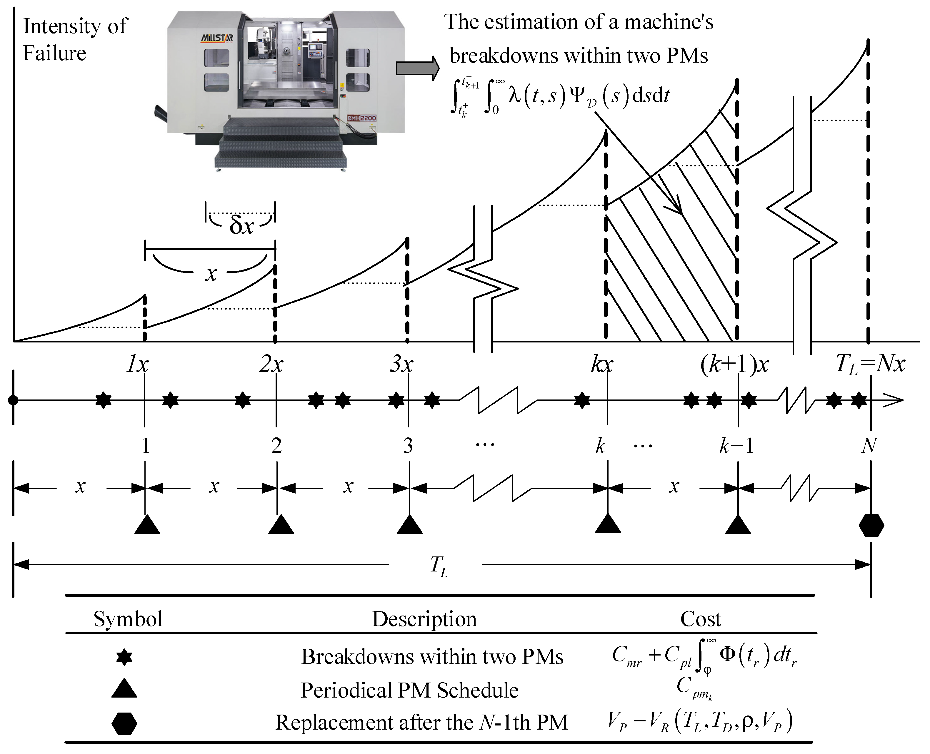
Suppose that the inter-PM time is set to $x$ according to the maintenance engineers’ suggestion. In order to evaluate the effective age of the system, the symbols $t_k^{-}$ and $t_k^{+}$ are used to denote the effective age before and after the kth PM action. We assume that the system can be partially recovered by a PM action and the degree of the recovery ${\delta }_{pm}^q$ can be measured by comparative deterioration experiments. The effective age of the system before the first PM action should be $t_1^{-}=x$. However, after the first PM action, the effective age of the system will be immediately recovered as $t_1^{+}=x-{\delta }_{pm}^{q}x=\left(1-{\delta }_{pm}^q\right)x$. Based on this, the effective ages of the system immediately before and after the kth PM action can be derived as

$$t_k^{-}=kx-\left(k-1\right){\delta }_{pm}^{q}x=\left(k-1\right)\left(1-{\delta }_{pm}^q\right)x+x=\left(\left(k-1\right)\left(1-{\delta }_{pm}^q\right)+1\right)x$$

(11)

and

$$t_k^{+}=t_k^{-}-{\delta }_{pm}^{q}x=kx-\left(k-1\right){\delta }_{pm}^{q}x-{\delta }_{pm}^{q}x=k\left(1-{\delta }_{pm}^q\right)x$$

(12)

respectively.

Figure 2 illustrates the timeline and breakdowns of a deteriorating system under the imperfect PM model.

During the lease period, the expected disbursement should include both the repair and preventive maintenance expenses. The concept of the repair cost consists of the two components: (1) the cost to perform a minimal repair ($C_{mr}$); (2) the penalty cost ($C_{pl}$) if the actual repair time exceed the tolerable waiting time $\phi$. Based on the lessor’s responsibility, any failure or breakdown of the lease product (facility or equipment) by the lessor’s maintenance department. Furthermore, the repair time $t_r$ can be thought of as a random variable with a Gamma probability distribution. The following equation presents the probability function that the repair time $t_r$ is over the time limit $\phi$.

$$\Phi \left(t_r\right)={{\displaystyle \int }}_{\phi }^{\infty }\frac{{\eta }^{\omega }{t}_r^{\omega -1}}{\Gamma \left(\omega \right)e^{\eta t_r}}d{t}_r$$

(13)

In order to estimate the probability of the overtime repair, it is necessary to evaluate the parameters $\omega$ and $\eta$ in advance. Since the parameters $\omega$ and $\eta$ are related to their expectation and variance, they can be calculated by $\omega =E{\left(t_r\right)}^2/\sigma {\left(t_r\right)}^2$ and $\eta =E\left(t_r\right)/\sigma {\left(t_r\right)}^2$.

In order to evaluate the repair cost of the lease facility or equipment, the lessor must estimate the facility or equipment’s deterioration over the lease period. Based on the assumption that the facility or equipment’s failure process is an NHPP with a specific intensity function $\lambda \left(t,s,\mathsf{\Theta }\right)$, the expected number of failures for the lease period $\left[0,T_L\right]$ under PM interval $x$ and age reduction $\delta$ is $E\left[N_{br}|T_L,x,{\delta }_q,{\mathsf{\Psi }}_{\mathcal{D}}\left(s\right),\mathsf{\Theta }\right]$. In accordance with the mentioned above, the total repair cost during the leasing period can be calculated as follows:

$$\left(C_{mr}+C_{pl}{{\displaystyle \int }}_{\phi }^{\infty }\Phi \left(t_r\right)d{t}_r\right)E\left[N_{br}|T_L,x,\delta ,{\Psi }_{\mathcal{D}}\left(s\right),\mathsf{\Theta }\right].$$

(14)

For preventive maintenance to be beneficial, the lessor should only perform it if the reduction of repair expense outweighs the maintenance cost. For sequential PM activities over the lease period, the maintenance costs will rise due to mechanical or electronic aging of the deteriorating system. According to Jayabalan and Chaudhuri [46], there is an approach to estimating maintenance costs per unit time during the lease period, and it can be calculated by:

$$C_{p{m}_k}=C_F\left(1+\tau \left(k-1\right)x\right)$$

(15)

where $C_F$ and $\tau$ respectively denote the base cost of proceeding with a PM and the increasing rate of the PM cost. As a result, the total PM cost should be given by

$$C_{pm}\left(C_F,\tau ,x,T_L\right)={\displaystyle \sum }_{k=1}^{T_L/x-1}{C}_{p{m}_k}={\displaystyle \sum }_{k=1}^{T_L/x-1}{C}_F\left(1+\tau (k-1\right)x).$$

(16)

In addition, various preventive maintenance options will influence the system’s recovery, but will also raise the lessor’s PM costs. Suppose that the series of PM alternatives $M_P=\left\{M_P^1,M_P^2,\dots M_P^q,\dots ,M_P^Q\right\}$ can be chosen, and the corresponding PM cost with the expected failure number can be rewritten as follows:

$$C_{pm}^q\left(C_F^q,{\tau }_q,x,T_L\right)={\displaystyle \sum }_{k=1}^{T_L/x-1}{C}_{p{m}_k}^q={\displaystyle \sum }_{k=1}^{T_L/x-1}{C}_F^q\left(1+{\tau }_q(k-1\right)x).$$

(17)

Accordingly, a failure of leased facility or equipment can be estimated based on the expected number during the lease period $T_L$ as follows:

$$\begin{array}{c}E\left[N_{br}|T_L,x,{\delta }_{pm}^q,{\Psi }_{\mathcal{D}}\left(s\right),\mathsf{\Theta }\right]\\ \hspace{1em}\hspace{1em}\hspace{1em}={{\displaystyle \int }}_{t_1^{+}}^{t_2^{-}}\left({{\displaystyle \int }}_0^{\infty }\lambda \left(t,s,\mathsf{\Theta }\right){\Psi }_{\mathcal{D}}\left(s\right)ds\right)dt+{{\displaystyle \int }}_{t_2^{+}}^{t_3^{-}}\left({{\displaystyle \int }}_0^{\infty }\lambda \left(t,s,\mathsf{\Theta }\right){\Psi }_{\mathcal{D}}\left(s\right)ds\right)dt+\dots \\ \hspace{1em}\hspace{1em}\hspace{1em}+{{\displaystyle \int }}_{t_k^{+}}^{t_{k+1}^{-}}\left({{\displaystyle \int }}_0^{\infty }\lambda \left(t,s,\mathsf{\Theta }\right){\Psi }_{\mathcal{D}}\left(s\right)ds\right)dt\\ \hspace{1em}\hspace{1em}\hspace{1em}\hspace{1em}={\displaystyle {\displaystyle \sum }_{k=1}^{T_L/x-1}}{{\displaystyle \int }}_{t_k^{+}}^{t_{k+1}^{-}}\left({{\displaystyle \int }}_0^{\infty }\lambda \left(t,s\right){\Psi }_{\mathcal{D}}\left(s\right)ds\right)dt\\ \hspace{1em}\hspace{1em}\hspace{1em}={\displaystyle {\displaystyle \sum }_{k=1}^{T_L/x-1}}{{\displaystyle \int }}_{kx}^{\left(k+1\right)x}\left({{\displaystyle \int }}_0^{\infty }\lambda \left(t-k{\delta }_{pm}^{q}x,s\right){\Psi }_{\mathcal{D}}\left(s\right)ds\right)dt.\end{array}$$

(18)

3. Optimal PM Decision to Facilities with and without Consideration of Financial Lease Contract Revenue

This section introduces the optimal decision of the multiple PM alternatives with and without considering a financial lease contract revenue. The proposed model can provide the best PM plan for lessors to reduce the related costs during the lease period by considering the lease revenue throughout the lease period and the residual value at the end. Furthermore, the analytical models and efficient solution algorithm will be provided for solving the issue of the leased facility with two-dimensional deterioration. Finally, in order to easily apply the models in a real scenario, a computerized system design is also proposed in this section.

3.1. Optimal PM without Consideration of Financial Lease Contract Revenue

Generally, the lessor not only provides lease facilities to customers (lessees) but also provides a free-repair warranty for increasing the customers’ satisfaction and reducing the related costs. Since a free-repair warranty would cover the costs of non-artificial damage or deterioration, the lessor must bear the expenses of repair, overtime, and preventive maintenance. Furthermore, due to the fact that the initial investment in lease facilities is the most significant expenditure for the lessor, he/her have to treat it as an amortized expenditure when calculating the average cost per unit of time, and the residual value of the lease facilities can be considered an investment deduction. However, if the lessor did not make the plan for the revenue of rent, the expected average cost per unit of time can be given by:

$$\begin{gathered} Min EC\left[N|M_P^q\right]=\frac{{{\displaystyle \sum }}_{k=1}^{T_L/x-1}{C}_{p{m}_k}^q+\left(C_{mr}+C_{pl}{{\displaystyle \int }}_{\phi }^{\infty }\Phi \left(t_r\right)d{t}_r\right)E\left[N_{br}|T_L,x,{\delta }_{pm}^q,{\Psi }_{\mathcal{D}}\left(s\right),\mathsf{\Theta }\right]+V_P}{T_L} \\ =\frac{{{\displaystyle \sum }}_{k=1}^{N-1}{C}_{p{m}_k}^q+\left(C_{mr}+C_{pl}{{\displaystyle \int }}_{\phi }^{\infty }\Phi \left(t_r\right)d{t}_r\right)E\left[N_{br}|T_L,x,{\delta }_{pm}^q,{\Psi }_{\mathcal{D}}\left(s\right),\mathsf{\Theta }\right]+V_P}{Nx}. \end{gathered}$$

(19)

The convexity of the cost function $EC\left[N|M_P^q\right]$ with respect to $N$ can be justified if the two inequalities $EC\left[N+1|M_P^q\right]\ge EC\left[N|M_P^q\right]$ and $EC\left[N|M_P^q\right]<EC\left[N-1|M_P^q\right]$ both hold, and the optimal $N^{*}$ can therefore be obtained.

Proposition 1.

If the intensity function$\lambda \left(t,s,\mathsf{\Theta }\right)$is strictly increasing, and the two inequalities$EC\left[N+1|M_P^q\right]\ge EC\left[N|M_P^q\right]$and$EC\left[N|M_P^q\right]<EC\left[N-1|M_P^q\right]$are both hold, the convexity of the cost function$EC\left[N|M_P^q\right]$with respect to N can be assured.

Proof: 

For $EC\left[N+1|M_P^q\right]\ge EC\left[N|M_P^q\right]$, we have $EC\left[N+1|M_P^q\right]-EC\left[N|M_P^q\right]\ge 0$

$$\begin{array}{c}\Rightarrow \frac{{{\displaystyle \sum }}_{k=1}^N{C}_{p{m}_k}^q+\left(C_{mr}+C_{pl}{{\displaystyle \int }}_{\phi }^{\infty }\mathsf{\Phi }\left(t_r\right)d{t}_r\right)E\left[N_{br}|\left(N+1\right)x,x,{\delta }_{pm}^q,{\mathsf{\Psi }}_{\mathcal{D}}\left(s\right),\mathsf{\Theta }\right]+V_P}{\left(N+1\right)x}\\ -\frac{{{\displaystyle \sum }}_{k=1}^{N-1}{C}_{p{m}_k}^q+\left(C_{mr}+C_{pl}{{\displaystyle \int }}_{\phi }^{\infty }\mathsf{\Phi }\left(t_r\right)d{t}_r\right)E\left[N_{br}|Nx,x,{\delta }_{pm}^q,{\mathsf{\Psi }}_{\mathcal{D}}\left(s\right),\mathsf{\Theta }\right]+V_P}{Nx}\ge 0\\ \Rightarrow \frac{{{\displaystyle \sum }}_{k=1}^N{C}_{p{m}_k}^q+\left(C_{mr}+C_{pl}{{\displaystyle \int }}_{\phi }^{\infty }\mathsf{\Phi }\left(t_r\right)d{t}_r\right)E\left[N_{br}|\left(N+1\right)x,x,{\delta }_{pm}^q,{\mathsf{\Psi }}_{\mathcal{D}}\left(s\right),\mathsf{\Theta }\right]+V_P}{\left(N+1\right)x}\\ -\frac{\left(\frac{N+1}{N}\right)\left\{{{\displaystyle \sum }}_{k=1}^{N-1}{C}_{p{m}_k}^q+\left(C_{mr}+C_{pl}{{\displaystyle \int }}_{\phi }^{\infty }\mathsf{\Phi }\left(t_r\right)d{t}_r\right)E\left[N_{br}|Nx,x,{\delta }_{pm}^q,{\mathsf{\Psi }}_{\mathcal{D}}\left(s\right),\mathsf{\Theta }\right]+V_P\right\}}{\left(N+1\right)x}\ge 0\\ \Rightarrow \frac{\left(C_{mr}+C_{pl}{{\displaystyle \int }}_{\phi }^{\infty }\mathsf{\Phi }\left(t_r\right)d{t}_r\right)\left\{E\left[N_{br}|\left(N+1\right)x,x,{\delta }_{pm}^q,{\mathsf{\Psi }}_{\mathcal{D}}\left(s\right),\mathsf{\Theta }\right]-\left(1+\frac{1}{N}\right)E\left[N_{br}|Nx,x,{\delta }_{pm}^q,{\mathsf{\Psi }}_{\mathcal{D}}\left(s\right),\mathsf{\Theta }\right]\right\}}{\left(N+1\right)x}\\ \hspace{1em}\hspace{1em}\ge \frac{\left(\frac{1}{N}\right)V_P-C_{p{m}_N}+\left(\frac{1}{N}\right){{\displaystyle \sum }}_{k=1}^{N-1}{C}_{p{m}_k}^q}{\left(N+1\right)x}\\ \hspace{1em}\hspace{1em}\Rightarrow \left(C_{mr}+C_{pl}{{\displaystyle \int }}_{\phi }^{\infty }\mathsf{\Phi }\left(t_r\right)d{t}_r\right)\{E\left[N_{br}|\left(N+1\right)x,x,{\delta }_{pm}^q,{\mathsf{\Psi }}_{\mathcal{D}}\left(s\right),\mathsf{\Theta }\right]\\ \hspace{1em}\hspace{1em}\hspace{1em}-\left(1+\frac{1}{N}\right)E\left[N_{br}|Nx,x,{\delta }_{pm}^q,{\mathsf{\Psi }}_{\mathcal{D}}\left(s\right),\mathsf{\Theta }\right]\}\ge \left(\frac{1}{N}\right)V_P-C_{p{m}_N}^q+\left(\frac{1}{N}\right){\displaystyle \sum }_{k=1}^{N-1}{C}_{p{m}_k}^q\\ \hspace{1em}\hspace{1em}\hspace{1em}\Rightarrow \left(C_{mr}+C_{pl}{{\displaystyle \int }}_{\phi }^{\infty }\mathsf{\Phi }\left(t_r\right)d{t}_r\right)\{E\left[N_{br}|\left(N+1\right)x,x,{\delta }_{pm}^q,{\mathsf{\Psi }}_{\mathcal{D}}\left(s\right),\mathsf{\Theta }\right]\\ \hspace{1em}\hspace{1em}\hspace{1em}-\left(N+1\right)E\left[N_{br}|Nx,x,{\delta }_{pm}^q,{\mathsf{\Psi }}_{\mathcal{D}}\left(s\right),\mathsf{\Theta }\right]\}\ge V_P-N{C}_{p{m}_N}^q+{\displaystyle \sum }_{k=1}^{N-1}{C}_{p{m}_k}^q\\ \hspace{1em}\hspace{1em}\Rightarrow NE\left[N_{br}|\left(N+1\right)x,x,{\delta }_{pm}^q,{\Psi }_{\mathcal{D}}\left(s\right),\mathsf{\Theta }\right]-\left(N+1\right)E\left[N_{br}|Nx,x,{\delta }_{pm}^q,{\Psi }_{\mathcal{D}}\left(s\right),\mathsf{\Theta }\right]\\ \hspace{1em}\hspace{1em}\hspace{1em}\ge \frac{V_P-N{C}_{p{m}_N}^q+{{\displaystyle \sum }}_{k=1}^{N-1}{C}_{p{m}_k}^q}{C_{mr}+C_{pl}{{\displaystyle \int }}_{\phi }^{\infty }\Phi \left(t_r\right)d{t}_r}\end{array}$$

(20)

For $EC\left[N|M_P^q\right]<EC\left[N-1|M_P^q\right]$, we have $EC\left[N|M_P^q\right])-EC\left[N-1|M_P^q\right]<0$

$$\begin{gathered} \Rightarrow \frac{{{\displaystyle \sum }}_{k=1}^{N-1}{C}_{p{m}_k}^q+\left(C_{mr}+C_{pl}{{\displaystyle \int }}_{\phi }^{\infty }\mathsf{\Phi }\left(t_r\right)d{t}_r\right)E\left[N_{br}|Nx,x,{\delta }_{pm}^q,{\mathsf{\Psi }}_{\mathcal{D}}\left(s\right),\mathsf{\Theta }\right]+V_P}{Nx} \\ \hspace{1em}-\frac{{{\displaystyle \sum }}_{k=1}^{N-2}{C}_{p{m}_k}^q+\left(C_{mr}+C_{pl}{{\displaystyle \int }}_{\phi }^{\infty }\mathsf{\Phi }\left(t_r\right)d{t}_r\right)E\left[N_{br}|\left(N-1\right)x,x,{\delta }_{pm}^q,{\mathsf{\Psi }}_{\mathcal{D}}\left(s\right),\mathsf{\Theta }\right]+V_P}{\left(N-1\right)x}<0 \end{gathered}$$

$$\hspace{1em}\Rightarrow \frac{\left(1-\frac{1}{N}\right)\left\{{{\displaystyle \sum }}_{k=1}^{N-1}{C}_{p{m}_k}^q+\left(C_{mr}+C_{pl}{{\displaystyle \int }}_{\phi }^{\infty }\mathsf{\Phi }\left(t_r\right)d{t}_r\right)E\left[N_{br}|Nx,x,{\delta }_{pm}^q,{\mathsf{\Psi }}_{\mathcal{D}}\left(s\right),\mathsf{\Theta }\right]+V_P\right\}}{\left(N-1\right)x}$$

$$\hspace{1em}-\frac{{{\displaystyle \sum }}_{k=1}^{N-2}{C}_{p{m}_k}^q+\left(C_{mr}+C_{pl}{{\displaystyle \int }}_{\phi }^{\infty }\mathsf{\Phi }\left(t_r\right)d{t}_r\right)E\left[N_{br}|\left(N-1\right)x,x,{\delta }_{pm}^q,{\mathsf{\Psi }}_{\mathcal{D}}\left(s\right),\mathsf{\Theta }\right]+V_P}{\left(N-1\right)x}<0$$

$$\begin{gathered} \hspace{1em}\Rightarrow \left(1-\frac{1}{N}\right){\displaystyle \sum }_{k=1}^{N-1}{C}_{p{m}_k}^q+\left(1-\frac{1}{N}\right)\left(C_{mr}+C_{pl}{{\displaystyle \int }}_{\phi }^{\infty }\mathsf{\Phi }\left(t_r\right)d{t}_r\right)E\left[N_{br}|Nx,x,{\delta }_{pm}^q,{\mathsf{\Psi }}_{\mathcal{D}}\left(s\right),\mathsf{\Theta }\right]+\left(1-\frac{1}{N}\right)V_P \\ \hspace{1em}\hspace{1em}-\left\{{\displaystyle \sum }_{k=1}^{N-2}{C}_{p{m}_k}^q+\left(C_{mr}+C_{pl}{{\displaystyle \int }}_{\phi }^{\infty }\mathsf{\Phi }\left(t_r\right)d{t}_r\right)E\left[N_{br}|\left(N-1\right)x,x,{\delta }_{pm}^q,{\mathsf{\Psi }}_{\mathcal{D}}\left(s\right),\mathsf{\Theta }\right]+V_P\right\}<0 \end{gathered}$$

$$\begin{gathered} \Rightarrow \left(C_{mr}+C_{pl}{{\displaystyle \int }}_{\phi }^{\infty }\mathsf{\Phi }\left(t_r\right)d{t}_r\right)\left\{\left(\frac{N-1}{N}\right)E\left[N_{br}|Nx,x,{\delta }_{pm}^q,{\mathsf{\Psi }}_{\mathcal{D}}\left(s\right),\mathsf{\Theta }\right]-E\left[N_{br}|\left(N-1\right)x,x,{\delta }_{pm}^q,{\mathsf{\Psi }}_{\mathcal{D}}\left(s\right),\mathsf{\Theta }\right]\right\} \\ \hspace{1em}+\left(\frac{N-1}{N}\right)C_{p{m}_{N-1}}^q-\left(\frac{1}{N}\right){\displaystyle \sum }_{k=1}^{N-2}{C}_{p{m}_k}^q-\left(\frac{1}{N}\right)V_P<0 \end{gathered}$$

$$\begin{gathered} \Rightarrow \left(C_{mr}+C_{pl}{{\displaystyle \int }}_{\phi }^{\infty }\mathsf{\Phi }\left(t_r\right)d{t}_r\right)\left\{\left(\frac{N-1}{N}\right)E\left[N_{br}|Nx,x,{\delta }_{pm}^q,{\mathsf{\Psi }}_{\mathcal{D}}\left(s\right),\mathsf{\Theta }\right]-E\left[N_{br}|\left(N-1\right)x,x,{\delta }_{pm}^q,{\mathsf{\Psi }}_{\mathcal{D}}\left(s\right),\mathsf{\Theta }\right]\right\} \\ \hspace{1em}+\left(\frac{N-1}{N}\right)C_{p{m}_{N-1}}^q-\left(\frac{1}{N}\right){\displaystyle \sum }_{k=1}^{N-2}{C}_{p{m}_k}^q-\left(\frac{1}{N}\right)V_P<0 \end{gathered}$$

$$\Rightarrow \left(N-1\right)E\left[N_{br}|Nx,x,{\delta }_{pm}^q,{\Psi }_{\mathcal{D}}\left(s\right),\Theta \right]-NE\left[N_{br}|\left(N-1\right)x,x,{\delta }_{pm}^q,{\Psi }_{\mathcal{D}}\left(s\right),\Theta \right]<\frac{V_P-\left(N-1\right)C_{p{m}_{N-1}}^q+{{\displaystyle \sum }}_{k=1}^{N-2}{C}_{p{m}_k}^q}{\left(C_{mr}+C_{pl}{{\displaystyle \int }}_{\phi }^{\infty }\Phi \left(t_r\right)d{t}_r\right)}$$

(21)

Let $\Delta \left(N\right)=NE\left[N_{br}|\left(N+1\right)x,x,{\delta }_q,{\mathsf{\Psi }}_{\mathcal{D}}\left(s\right),\mathsf{\Theta }\right]-\left(N+1\right)E\left[N_{br}|Nx,x,{\delta }_q,{\mathsf{\Psi }}_{\mathcal{D}}\left(s\right),\mathsf{\Theta }\right]$ for $N\in Z^{+}$ and $\Delta \left(N\right)$ = 0 for $N$ = 0. Since $\Delta \left(N\right)$ is strictly increasing, it exists an $N$ such that inequalities (20) and (21) would hold simultaneously, and such an $N$ is the optimal number of periodic PM actions. Since the failure rate is increasing over time for deteriorating systems, i.e., $\lambda \left(t,s,\mathsf{\Theta }\right)>\lambda \left(0,s,\mathsf{\Theta }\right)$ for $t>0$, we then have $\Delta \left(N\right)-\Delta \left(N-1\right)=N\left\{\left(E\left[N_{br}|\left(N+1\right)x,x,{\delta }_{pm}^q,{\mathsf{\Psi }}_{\mathcal{D}}\left(s\right),\mathsf{\Theta }\right]-E\left[N_{br}|Nx,x,{\delta }_{pm}^q,{\mathsf{\Psi }}_{\mathcal{D}}\left(s\right),\mathsf{\Theta }\right]\right)-\left(E\left[N_{br}|Nx,x,{\delta }_{pm}^q,{\mathsf{\Psi }}_{\mathcal{D}}\left(s\right),\mathsf{\Theta }\right]-E\left[N_{br}|\left(N-1\right)x,x,{\delta }_{pm}^q,{\mathsf{\Psi }}_{\mathcal{D}}\left(s\right),\mathsf{\Theta }\right]\right)\right\}>0$, and the convexity of the cost function $E\left[N_{br}|Nx,x,{\delta }_q,{\mathsf{\Psi }}_{\mathcal{D}}\left(s\right),\mathsf{\Theta }\right]$ with respect to $N$ is thus assured.

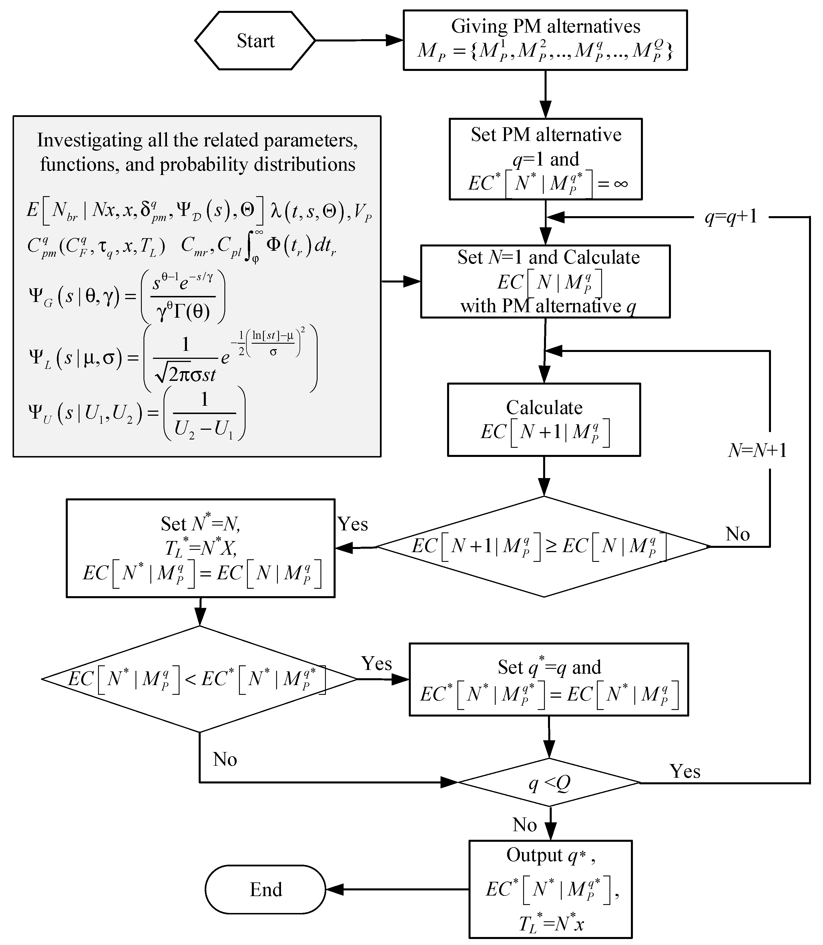
Based on Proposition 1, the heuristic solution algorithm for obtaining the optimal cost can be briefly presented as follows:

• Step 1: Initially, all the PM alternatives are given as the candidate list $M_P=\left\{M_P^1,M_P^2,\dots M_P^q,\dots ,M_P^Q\right\}$.
• Step 2: Start with the first PM alternative ($q=1$), and the variable of the optimal expected cost $E{C}^{*}\left[N^{*}|M_P^{q^{*}}\right]$ is set to infinity.
• Step 3: Set the PM number $N=1$ and calculate the expected cost $EC\left[N|M_P^q\right]$.
• Step 4: Calculate the expected cost $EC\left[N+1|M_P^q\right]$.
• Step 5: Investigating whether the condition $EC\left[N+1|M_P^q\right]\ge EC\left[N|M_P^q\right]$ is supported or not? If it is supported, go to Step 6. Otherwise, go to Step 4 with $N\leftarrow N+1$.
• Step 6: Set the optimal number as $N^{*}\leftarrow N$, the optimal lease length as $T_L^{*}\leftarrow N^{*}x$, and the variable of the optimal expected cost as $E{C}^{*}\left[N^{*}|M_P^q\right]\leftarrow EC\left[N|M_P^q\right]$.
• Step 7: Investigating whether the condition $E{C}^{*}\left[N^{*}|M_P^q\right]<E{C}^{*}\left[N^{*}|M_P^{q^{*}}\right]$ is supported or not? If the answer is yes, go to Step 8. Otherwise, go to Step 9.
• Step 8: Set the optimal PM alternative as $q^{*}\leftarrow q$ and the variable of the optimal expected cost as $E{C}^{*}\left[N^{*}|M_P^{q^{*}}\right]\leftarrow E{C}^{*}\left[N^{*}|M_P^q\right]$.
• Step 9: Investigating whether the condition $q<Q$ has reached? If the answer is yes, go to Step 3 with $q\leftarrow q+1$. Otherwise, go to Step 10.
• Step 10: Output the optimal solution (The best PM alternative $q^{*}$, the optimal expected cost $E{C}^{*}\left[N^{*}|M_P^{q^{*}}\right]$, the optimal lease length $T_L^{*}$) $EC\left[N+1|M_P^q\right]\ge EC\left[N|M_P^q\right]$.

The above solution algorithm is illustrated in Figure 3.

3.2. Optimal PM with Consideration of Financial Lease Contract Revenue

As a result of some financial considerations, a company may rent some facilities instead of buying them. In order to increase customers’ satisfaction, the lessor will provide a free repair warranty on the lease contract. In order to effectively control the frequency of facility breakdowns and reduce the repair cost, the lessor has to make effective PM alternatives. In the previous section, the lessor only pursues the optimization from the cost perspective. However, there is no guarantee that low costs will lead to high profits. It depends on the lease revenue of the lease contract and the compensation of the residual value. Taking the revenue into account, the rent is $R\left(T_L,T_D,\overline{R},\xi \right)$ with the discount rate $\xi$ during the lease period $T_L$. Suppose that the rent of each period $T_D$ is $\overline{R}$. The payment of the lease facilities can be evaluated as follows:

$$R\left(T_L,T_D,\overline{R},\xi \right)=\overline{R}+\overline{R}\left(1-\xi \right)+\overline{R}{\left(1-\xi \right)}^2+\cdots +\overline{R}{\left(1-\xi \right)}^{T_L/T_D-1}=\overline{R}\left(\frac{1-{\left(1-\xi \right)}^{T_L/T_D}}{\xi }\right).$$

(22)

In addition, the lessor may sell the old leased facility to retrieve a part of the original investment at the end of the lease period, as a result, the firm needs to estimate or evaluate the residual value of the leased facility. In other word, the residual value of a leased facility can be regarded as of a part of the revenue of the lease contract. In this study, a declining balance depreciation method is used to evaluate the residual value since the method is popular in most accounting systems. Based on the above-mentioned, the estimated residual value of the leased facility can be formulated as follow:

$$V_R\left(T_L,T_D,\rho ,V_P\right)=V_P{\left(1-\rho \right)}^{T_L/T_D},$$

(23)

In Equation (23), $\rho$ is the depreciation rate of the leased facility after a time segment (year). Accordingly, the lessor’s profit can be formulated as follow:

$$\begin{array}{c}Max E\left[\pi |T_L,M_P^q\right]\\ =\left(\frac{1}{T_L}\right)\{R\left(T_L,T_D,\overline{R},\xi \right)+V_R\left(T_L,T_D,\rho ,V_P\right)-C_{pm}^q\left(C_F^q,{\tau }_q,x,T_L\right)\\ -\left(C_{mr}+C_{pl}{{\displaystyle \int }}_{\phi }^{\infty }\Phi \left(t_r\right)d{t}_r\right)E\left[N_{br}|T_L,x,{\delta }_q,{\Psi }_{\mathcal{D}}\left(s\right),\mathsf{\Theta }\right]-V_P\}\\ Subject to: T_L^{LB}\le T_L\le T_L^{UB}\end{array}$$

(24)

$T_L^{UB}$ and $T_L^{LB}$ denote the upper and lower bounds of the leased facility’s lifetime, and the length of lease contract can’t exceed the leased facility’s lifetime. Accordingly, the heuristic solution algorithm for obtaining the optimal cost can be briefly presented as follows:

Step 1: Initially, all the PM alternatives are given as the candidate list $M_P=\left\{M_P^1,M_P^2,\dots M_P^q,\dots ,M_P^Q\right\}$ and set the variable $E^{*}\left[\pi |T_L^{*},M_P^{q^{*}}\right]\leftarrow -\infty$.

Step 2: Start with the first PM alternative ($q=1$), and set $T_L\leftarrow T_L^{LB}$, $N\leftarrow T_L/x$, and $E^{*}\left[\pi |T_L^{*},M_P^q\right]\leftarrow -\infty$.

Step 3: Calculate the expected profit $E\left[\pi |T_L,M_P^q\right]$ under the lease period $T_L$ and the PM alternative $M_P^q$.

Step 4: Investigating whether the condition $E\left[\pi |T_L,M_P^q\right]\ge E^{*}\left[\pi |T_L^{*},M_P^q\right]$ is supported or not? If it is supported, go to Step 5. Otherwise, go to Step 6.

Step 5: Set $E^{*}\left[\pi |T_L^{*},M_P^q\right]\leftarrow E\left[\pi |T_L,M_P^q\right]$ and $T_L^{*}\leftarrow T_L$.

Step 6: Investigating whether the condition $T_L<T_L^{UB}$ has reached or not? If yes, calculate $T_L\leftarrow T_L+x$ and $N\leftarrow N+1$, and then go to Step 3. Otherwise, go to Step 7.

Step 7: Investigating whether the condition $E^{*}\left[\pi |T_L^{*},M_P^q\right]>E^{*}\left[\pi |T_L^{*},M_P^{q^{*}}\right]$ is supported or not? If it is supported, go to Step 8. Otherwise, go to Step 9.

Step 8: Set $q^{*}\leftarrow q$ and $E^{*}\left[\pi |T_L^{*},M_P^{q^{*}}\right]\leftarrow E^{*}\left[\pi |T_L^{*},M_P^q\right]$.

Step 9: Investigating whether the condition $q<Q$ has reached or not? If yes, set $q\leftarrow q+1$ and then go to Step 2. Otherwise, go to Step 10.

Step 10: Output the optimal solution (The best PM alternative $q^{*}$, the optimal lease length $T_L^{*}$, the optimal expected profit $E^{*}\left[\pi |T_L^{*},M_P^{q^{*}}\right]$)

The above solution algorithm can be illustrated as Figure 4.

3.3. Computerized Decision Support System Design

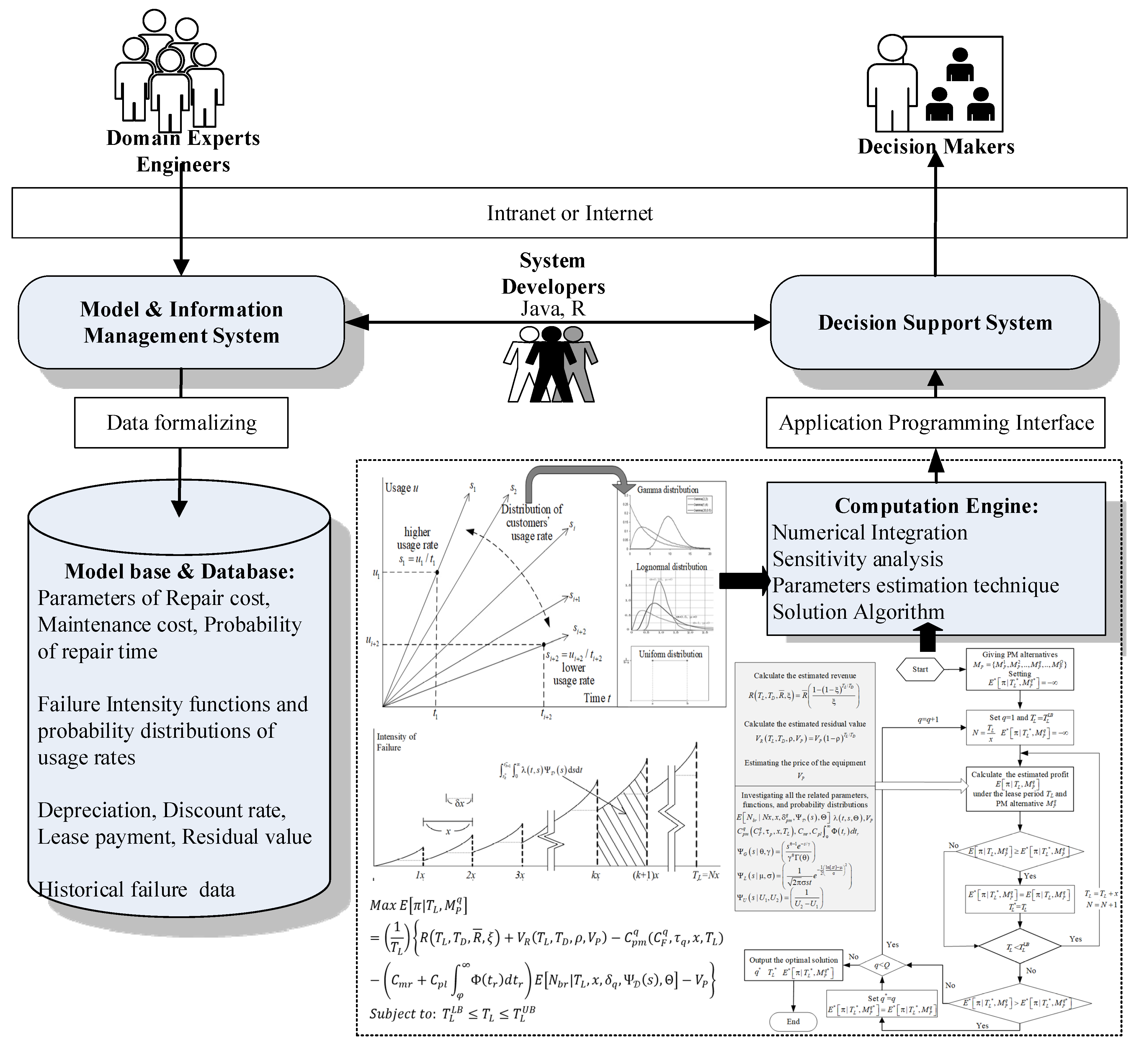
To obtain the optimal decision in such complicated mathematical problems, a computerized application would be required. In order to enhance the manageability of the whole application, it can be designed as the two independent systems (the model and information management system and the decision support system). The model and information management system is mainly used to store the failure datasets to estimate the values of deteriorating model parameters. Furthermore, the different PM alternatives’ parameters’ values, customers’ usage patterns, the corresponding probability distributions, and all the related costs and revenues are also critical to the cost or profit analyses. In order to store and retrieve all the information more conveniently and efficiently, the system developers have to design a data formalization mechanism, and it might be different from a traditional relational database because some data present hierarchical structure. After investigating and obtaining all the required information, the firm’s domain experts and engineers can use the model and information management system to store, retrieve, maintain, and analyze them. Moreover, in order to provide useful information and suggestion to the firm’s managers, the decision support system is required in practice. In order to deal with the estimation of parameters, solution algorithm, numeric integration, graphic presentation, and sensitivity analyses, computation engines will be needed for analyzing all the candidate alternatives. Such computation engines can be developed by the R projects’ package, and the system developers/programmers can write Java codes to apply them through an application programming interface (API). The computerized implementation architecture of our system is shown in Figure 5.

4. Application and Sensitivity Analysis

4.1. Application

Assume an industrial equipment maker (lessor) proposes a capital leasing project to attract consumers in the industrial equipment market since most companies or organizations prefer to lease rather than buy for financial and tax reasons. During the lease period, the industrial equipment maker will provide a preventive maintenance and free repair service to consumers (lessee). Due to the fact that the machinery equipment’s deterioration is not only influenced by time but also influenced by usage, the domain experts and engineers will evaluate the characteristics of the machine’s degradation. After the evaluation, the domain experts and engineers consider that the machine’s deterioration will follow the bivariate Weibull process, and its model parameters can be estimated from the historical data which was produced by some accelerated deterioration experiments. Besides, the lessees are heterogeneous due to their custom and usage. We assume that the lessees usage rates $s$ may follow a Gamma distribution with $E\left(s\right)=1.5$ and $\sigma {\left(s\right)}^2=0.7$.

Furthermore, since the repair time is not constant and it will be influenced by the degree of a machine’s breakdown, the repair time is need to be estimated first. However, the time for some repair works may exceed the tolerable limit due to serious breakdowns, and it will cause the increase in the penalty cost. The probability of the repair time over the tolerable limit can be evaluated by the reliability engineers. After the evaluation, the expected value $E\left(t_r\right)$ and standard deviation $\sigma \left(t_r\right)$ of performing a repair are estimated as 9 h and 5 h, respectively.

Moreover, the reliability engineers recommend six distinct PM alternatives, each of which will result in different expenditures and systems’ recovery during the lease period. Although alternative 6’s age reduction factor is greater than the other alternatives, its PM cost and increasing rate are also higher than the others. As a result, determining which PM alternative is preferable for the lessor is difficult. Because the lease length of the contract has an influence on the revenue, residual value, and associated costs, the lessor should carefully choose a PM alternative and the lease length to optimize its average profit. Based on the foregoing,

Table 2. The detailed information of the candidate PM alternatives.

The estimated values of the parameters of the two-dimensional deterioration	$\alpha =1.1$, $\beta =1.4$, $\omega =1.25$, $\kappa =1.65$
Interval of PM; Time segment	$x=0.5\mathrm{years}$; $T_D=0.5\mathrm{years}$
The probability distribution of customers’ usage rate	Gamma probability distribution ${\mathsf{\Psi }}_G\left(s|\theta ,\gamma \right)=\left(\frac{s^{\theta -1}{e}^{-s/\gamma }}{{\gamma }^{\theta }\mathsf{\Gamma }\left(\theta \right)}\right)$ with $E\left(s\right)=1.5$ and $\sigma {\left(s\right)}^2=0.7$
Age reduction factors of the alternatives (1..6)	${\delta }_{pm}^q=\left\{0.6,0.65,0.7,0.75,0.8,0.85\right\}$
The base cost for a PM action (1..6)	$C_F^q=\left\{\$570,\$650,\$700,\$730,\$750,\$820\right\}$
Periodically increasing rates of PM cost (1..6)	${\tau }_q=\left\{0.08,0.09,0.12,0.125,0.135,0.15\right\}$
Depreciation rate	$\rho =0.15$
The lower and upper boundaries of the planned lease terms	$T_L^{LB}=2 \mathrm{years}$; $T_L^{UB}=15 \mathrm{years}$
Rental per half-year	$\overline{R}=\$9800$
Time discount rate	$\xi =0.02$
The purchasing cost of an equipment	$V_P=\$90,000$
Expected cost of performing a minimal repair	$C_{mr}$ = $450
Penalty cost when the repair time exceed the time limit $\phi$	$C_{pl}=\$250$
Expected value and standard deviation of performing a minimal repair	$E\left(t_r\right)=9\mathrm{h}$, $\sigma \left(t_r\right)=5\mathrm{h}$
Tolerable waiting time limit for performing a minimal repair	$\phi =4.5\mathrm{h}$

presents thorough information on the six PM alternatives, together with expert evaluations on the leasing equipment’s deterioration.

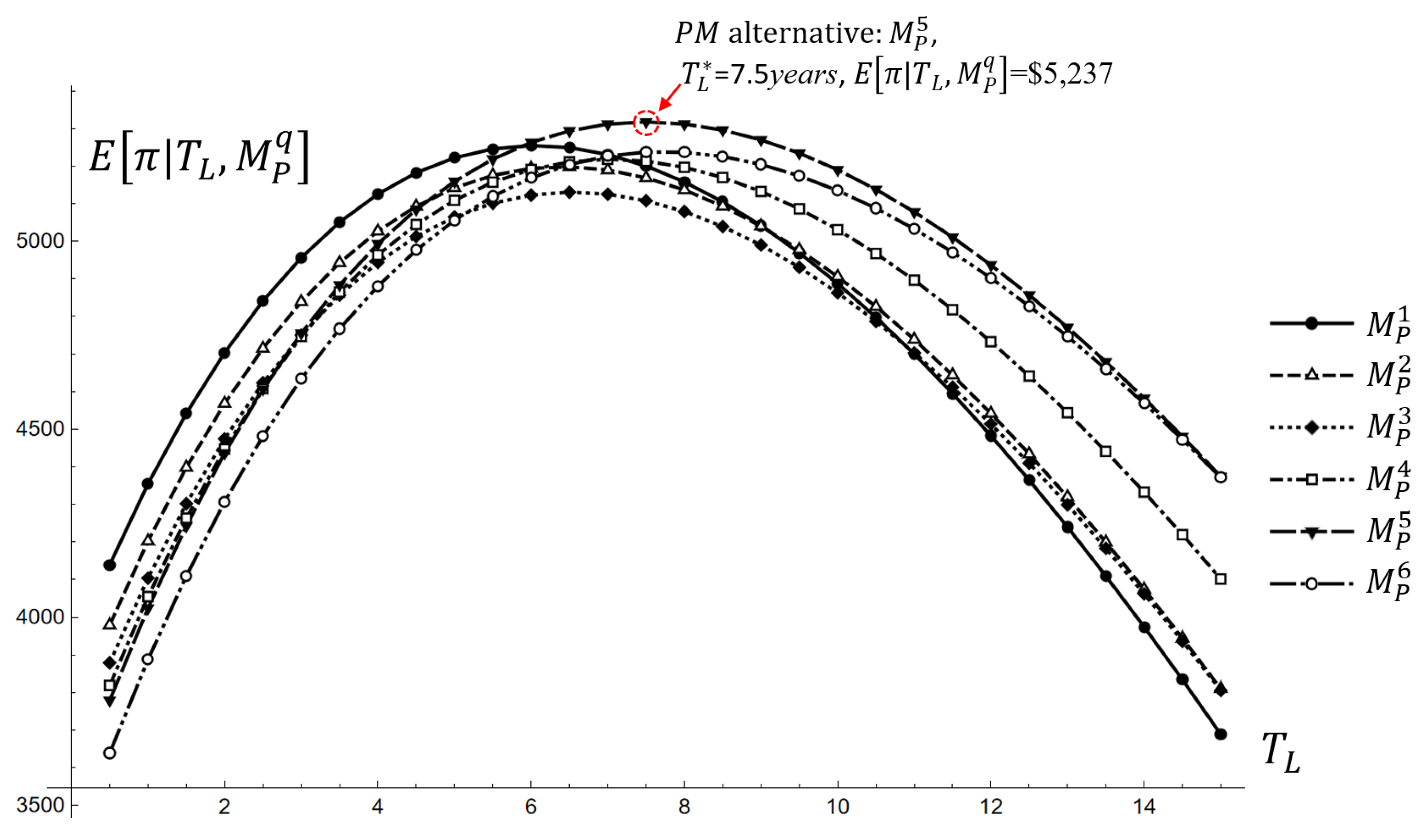
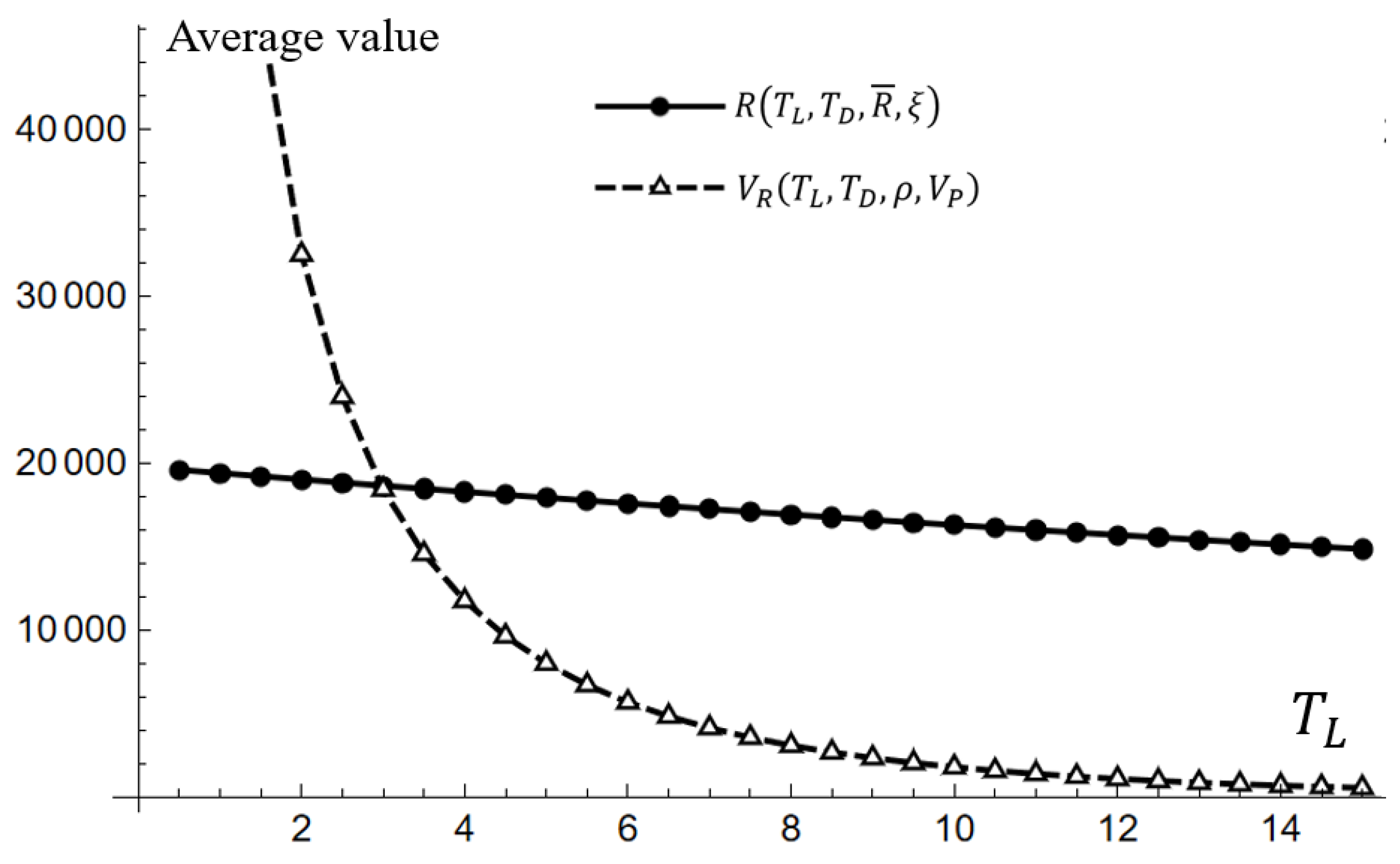
After performing the proposed heuristic algorithm presented in Figure 4, the numerical results are shown in Figure 6. According to

Table 3. Average residual value, related costs and profit per unit and year for the PM alternatives.

${\mathit{T}}_{\mathit{L}}$	${\mathit{V}}_{\mathit{R}}\left({\mathit{T}}_{\mathit{L}}\right)$	${\mathit{C}}_{\mathit{p}\mathit{m}}^{\mathit{q}}\left({\mathit{C}}_{\mathit{F}}^{\mathit{q}},{\mathit{\tau }}_{\mathit{q}},\mathit{x},{\mathit{T}}_{\mathit{L}}\right)$						$({\mathit{C}}_{\mathit{m}\mathit{r}}+{\mathit{C}}_{\mathit{p}\mathit{l}}{{\displaystyle \int }}_{\mathit{\phi }}^{\mathit{\infty }}\mathbf{\Phi }\left({\mathit{t}}_{\mathit{r}}\right)\mathit{d}{\mathit{t}}_{\mathit{r}})\mathit{E}\left[{\mathit{N}}_{\mathit{b}\mathit{r}}\right]$						$\mathit{E}\left[\mathit{\pi }|{\mathit{T}}_{\mathit{L}},{\mathit{M}}_{\mathit{P}}^{\mathit{q}}\right]$
		${\mathit{M}}_{\mathit{P}}^1$	${\mathit{M}}_{\mathit{P}}^2$	${\mathit{M}}_{\mathit{P}}^3$	${\mathit{M}}_{\mathit{P}}^4$	${\mathit{M}}_{\mathit{P}}^5$	${\mathit{M}}_{\mathit{P}}^6$	${\mathit{M}}_{\mathit{P}}^1$	${\mathit{M}}_{\mathit{P}}^2$	${\mathit{M}}_{\mathit{P}}^3$	${\mathit{M}}_{\mathit{P}}^4$	${\mathit{M}}_{\mathit{P}}^5$	${\mathit{M}}_{\mathit{P}}^6$	${\mathit{M}}_{\mathit{P}}^1$	${\mathit{M}}_{\mathit{P}}^2$	${\mathit{M}}_{\mathit{P}}^3$	${\mathit{M}}_{\mathit{P}}^4$	${\mathit{M}}_{\mathit{P}}^5$	${\mathit{M}}_{\mathit{P}}^6$
2	32,513	1208	1388	1526	1597	1652	1825	621	576	532	488	444	401	4703	4568	4474	4447	4436	4307
2.5	23,980	1231	1417	1568	1643	1703	1886	740	680	620	561	503	444	4841	4715	4623	4608	4607	4481
3	18,424	1254	1446	1610	1688	1753	1948	860	784	709	635	561	488	4956	4839	4750	4746	4755	4634
3.5	14,559	1277	1476	1652	1734	1804	2009	980	889	799	709	620	532	5050	4943	4856	4864	4884	4767
4	11,745	1300	1505	1694	1779	1854	2071	1102	995	889	784	679	576	5125	5027	4943	4963	4993	4880
4.5	9625	1322	1534	1736	1825	1905	2132	1224	1101	980	859	739	620	5182	5093	5013	5044	5084	4976
5	7987	1345	1563	1778	1871	1956	2194	1347	1208	1071	934	799	664	5222	5142	5065	5109	5159	5056
5.5	6694	1368	1593	1820	1916	2006	2255	1470	1316	1162	1010	859	709	5246	5175	5101	5157	5218	5119
6	5657	1391	1622	1862	1962	2057	2317	1594	1423	1254	1086	919	754	5254	5194	5123	5191	5263	5169
6.5	4815	1414	1651	1904	2008	2108	2378	1718	1531	1346	1162	979	798	5249	5198	5130	5211	5294	5204
7	4122	1436	1680	1946	2053	2158	2440	1843	1640	1438	1238	1040	843	5231	5190	5125	5218	5312	5227
7.5	3547	1459	1710	1988	2099	2209	2501	1968	1749	1531	1315	1101	889	5200	5169	5108	5213	5317	5237
8	3066	1482	1739	2030	2144	2259	2563	2093	1858	1624	1392	1162	934	5158	5136	5079	5197	5312	5237
8.5	2660	1505	1768	2072	2190	2310	2624	2219	1967	1717	1469	1223	979	5105	5093	5039	5169	5296	5225
9	2316	1528	1797	2114	2236	2361	2686	2345	2077	1811	1546	1284	1025	5042	5040	4990	5132	5270	5204
9.5	2023	1550	1827	2156	2281	2411	2747	2472	2187	1904	1624	1346	1070	4969	4977	4931	5086	5234	5174
10	1772	1573	1856	2198	2327	2462	2809	2599	2298	1998	1701	1407	1116	4887	4906	4863	5031	5190	5135
10.5	1556	1596	1885	2240	2373	2513	2870	2726	2408	2093	1779	1469	1162	4797	4826	4787	4967	5138	5088
11	1369	1619	1914	2282	2418	2563	2932	2853	2519	2187	1857	1531	1207	4700	4738	4703	4896	5078	5033
11.5	1207	1642	1944	2324	2464	2614	2993	2981	2630	2281	1935	1593	1253	4595	4644	4612	4818	5011	4971
12	1067	1664	1973	2366	2509	2664	3055	3109	2741	2376	2014	1655	1299	4483	4542	4514	4733	4937	4902
12.5	944	1687	2002	2408	2555	2715	3116	3237	2853	2471	2092	1717	1345	4364	4434	4409	4641	4857	4827
13	837	1710	2031	2450	2601	2766	3178	3365	2964	2566	2171	1779	1391	4240	4319	4299	4544	4771	4746
13.5	743	1733	2061	2492	2646	2816	3239	3494	3076	2661	2250	1841	1438	4110	4200	4183	4441	4679	4660
14	661	1756	2090	2534	2692	2867	3301	3623	3188	2757	2328	1904	1484	3974	4075	4062	4333	4582	4568
14.5	588	1778	2119	2576	2738	2918	3362	3752	3301	2852	2408	1967	1530	3834	3945	3936	4219	4480	4472
15	524	1801	2148	2618	2783	2968	3424	3881	3413	2948	2487	2029	1577	3689	3810	3805	4102	4374	4371

, the ideal lease lengths for the six PM alternatives should be 6, 6.5 6.5, 7, 7.5, and 7.5 years, with average earnings of $5254, $5198, $5130, $5217, $5317, and $5237 per unit. It is obvious that PM alternative 5 is the best option for the lessor, and the optimal lease length is about 7.5 years. As a result, it can be observed that the extremely intensive PM alternative may not have a positive influence on earnings. In general, the highest intensive PM alternatives can lower failure times while saving money on repairs. However, the cost savings from repairs cannot fully remedy the increase in PM costs. According to Table 3, we can see that the profit of PM alternative 6 is lower than that of PM alternatives 1 and 4. Accordingly, it is difficult to judge which PM alternative is best by intuition. Although a lower-intensive PM alternative will result in major failures during the post-phase, the lessor can avoid this disadvantage by opting for a shorter lease period if the lessor is subject to accepting a lower-intensive PM alternative due to the lack of critical replaceable components. It can be seen that once the lease length exceeds 6 years, the average profit of PM alternative 5 is higher than that of the other alternatives. However, before the time point, PM alternative 5 is not always more advantageous than others. Accordingly, if the lessor needs to shorten the lease length for some reason, PM alternative 1 (lowest intensive PM) will be the best choice for less than six years. For example, the customers may not accept a long-term lease contract, and therefore the lessor can make an appropriate contract with different customers through negotiation. Besides, from the aspect of the expenditures, the optimal lease length may be longer than 7.5 years because the average of the accumulated depreciation ($\left(V_P-V_R\left(T_L,T_D,\rho ,V_P\right)\right)/T_L$) presents a rapidly increasing trend before 9 years in Figure 7. Accordingly, different aspects will influence the lessor to make different decisions.

4.2. Sensitivity Analysis

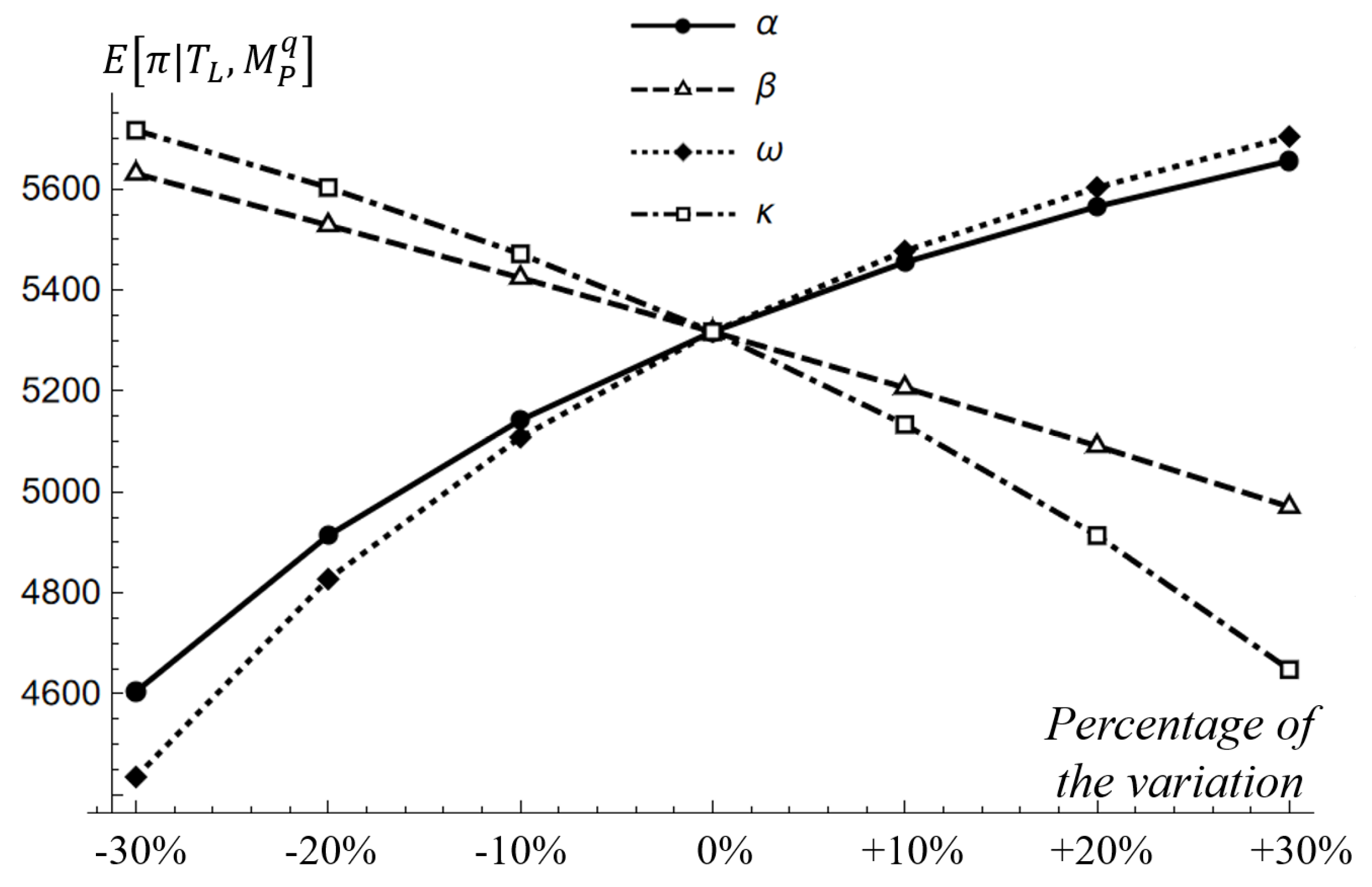
The estimation of the scale and shape parameters $\alpha$, $\omega$, $\beta$ and $\kappa$ may be inaccurate due to insufficient data from deterioration experiments. Therefore, the inaccurate estimation will have an influence on the prediction of the average profit and related costs, thus the lessor should be aware of any changes in the estimations. As a result, sensitivity analysis can be used to assess differences in estimated average profit. Furthermore, it is logical to assume that if we underestimate these parameters’ value, the estimated repair cost will also be inaccurate and it leads to incorrect decisions such as incorrectly extending or shortening the lease length. Figure 8 presents the impact of the scale and shape parameters $\alpha$, $\omega$, $\beta$ and $\kappa$ on the expected profit. According to Figure 8, if the scale parameters $\alpha$ and $\omega$ are estimated to be larger, the profits are also estimated to be amplified because the number of breakdowns is underestimated. On the contrary, the overestimation of the shape parameters $\beta$ and $\kappa$ would cause the underestimation of the estimated profit. Moreover, the impact of the parameters regarding usage ($\omega ,\kappa$) is more than that of the parameters regarding time ($\alpha ,\beta$). In other words, the deterioration of usage is more than that of time, and the lessor should pay attention to the improvement of the related usage components to mitigate the deterioration.

Furthermore, since the variation of the related costs and the parameters of PM might impact the expected profit and the decision-making, the lessor should be aware of any changes in the related costs. Figure 9 depicts the impact of the parameters $C_{mr}$, $C_{pl}$, $C_F^q$ and ${\tau }_q$ on the expected profit. According to Figure 9, the base cost of PM ($C_F^q$) is more sensitive than the repair cost and the penalty cost. It is because the lessor takes a high intensive PM alternative, and such high intensive PM can effectively reduce the repair and penalty cost but it also increases the lessor’s PM cost. Accordingly, the lessor must balance the two costs to make the best decision. Moreover, the lessor should also consider to shortening the lease length to respond to the increase of repair and penalty costs when the lessor adopted a low intensive PM alternative. Besides, the growing rate of PM cost may rise due to the inflation of linked prices. The impact will be increased as the lease length increases. Accordingly, as the base cost of PM rises, the optimal lease length should be shortened to reduce the burden of PM costs.

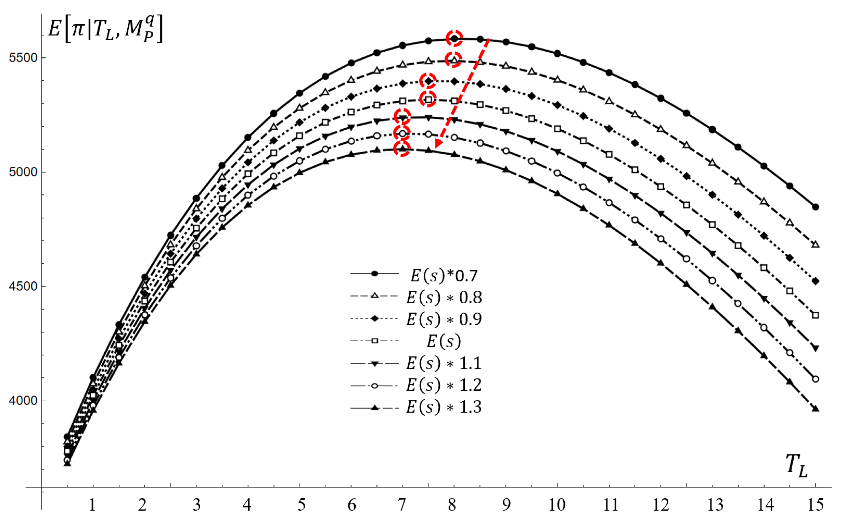
Since different customers (lessees) have their individual needs or usage style, their lease facility will present different deteriorations and different numbers of failures under the same lease length. For measuring the impact of these different customers on the facility’s deterioration, the usage rate is a useful indicator for calculating the different customers’ lease facility breakdowns. Figure 10 depicts the impact of the customers’ average usage rate on the expected profit. In this case, the usage rate is assumed to be a Gamma distribution with $E\left(s\right)=1.5$ and $\sigma {\left(s\right)}^2=0.7$. According to Figure 10, if $E\left(s\right)$ is higher, the lease length should be shortened for obtaining the optimal expected profit. According to the information in

Table 4. The impact of $E\left(s\right)$ and $\sigma {\left(s\right)}^2$ on expected profit.

${\mathit{T}}_{\mathit{L}}$	$\mathit{E}\left(\mathit{s}\right)$							$\mathit{\sigma }{\left(\mathit{s}\right)}^2$
	−30%	−20%	−10%	0%	+10%	+20%	+30%	−30%	−20%	−10%	0%	+10%	+20%	+30%
2	4540	4503	4469	4436	4405	4375	4346	4432	4433	4435	4436	4438	4439	4441
2.5	4724	4682	4644	4607	4571	4537	4505	4601	4603	4605	4607	4608	4610	4612
3	4886	4840	4797	4755	4716	4678	4642	4749	4751	4753	4755	4757	4759	4761
3.5	5029	4977	4929	4884	4840	4798	4758	4877	4879	4881	4884	4886	4888	4890
4	5152	5096	5043	4993	4945	4899	4855	4986	4988	4991	4993	4995	4998	5000
4.5	5257	5196	5139	5084	5033	4983	4935	5077	5079	5082	5084	5087	5089	5092
5	5346	5280	5218	5159	5103	5049	4997	5151	5154	5157	5159	5162	5165	5167
5.5	5419	5348	5282	5218	5158	5100	5044	5210	5213	5215	5218	5221	5224	5227
6	5478	5402	5331	5263	5198	5136	5077	5253	5257	5260	5263	5266	5269	5272
6.5	5523	5442	5366	5294	5225	5159	5095	5284	5287	5290	5294	5297	5300	5304
7	5555	5469	5388	5312	5238	5168	5101	5301	5304	5308	5312	5315	5319	5322
7.5	5575	5484	5398	5317	5240	5166	5094	5306	5310	5314	5317	5321	5325	5328
8	5583	5487	5397	5312	5230	5152	5076	5300	5304	5308	5312	5316	5320	5323
8.5	5581	5480	5386	5296	5210	5127	5048	5283	5287	5292	5296	5300	5304	5308
9	5570	5464	5364	5270	5179	5093	5009	5256	5261	5265	5270	5274	5278	5283
9.5	5549	5438	5333	5234	5140	5049	4962	5220	5225	5230	5234	5239	5243	5248
10	5519	5403	5294	5190	5091	4996	4905	5176	5180	5185	5190	5195	5200	5204
10.5	5481	5360	5246	5138	5035	4936	4840	5123	5128	5133	5138	5143	5148	5153
11	5436	5309	5190	5078	4970	4867	4768	5062	5067	5073	5078	5083	5088	5093
11.5	5383	5251	5128	5011	4899	4791	4688	4994	5000	5005	5011	5016	5021	5027
12	5323	5187	5059	4937	4821	4709	4601	4920	4925	4931	4937	4942	4948	4953
12.5	5258	5116	4983	4857	4736	4620	4509	4839	4845	4851	4857	4862	4868	4874
13	5186	5039	4901	4771	4646	4526	4410	4752	4758	4764	4771	4777	4783	4788
13.5	5109	4957	4814	4679	4550	4425	4306	4660	4666	4673	4679	4685	4691	4697
14	5027	4870	4722	4582	4448	4320	4196	4562	4569	4576	4582	4589	4595	4601
14.5	4940	4778	4625	4480	4342	4210	4082	4460	4467	4474	4480	4487	4494	4500
15	4849	4681	4524	4374	4232	4095	3963	4353	4360	4367	4374	4381	4388	4395

, we can see −30%~+30% of $E\left(s\right)$ to map to the optimal lease lengths 8, 8, 7.5, 7.5, 7, 7, 7 years to obtain the profits $5583, $5487, $5398, $5317, $5238, $5168, $5101. This sensitive result reflects that the degree of usage deterioration is higher than the degree of time deterioration in this case. However, the impact of $\sigma \left(s\right)$ on the expected profit seems insensitive, and therefore the variation of $\sigma \left(s\right)$ would not change the decision of the lease length in this case.

5. Conclusions

For the purpose of this study, we provide analytical models and to provide efficient solution algorithms for solving the problem of two-dimensional deterioration in leased facilities. As a result of the proposed model, a PM scheme can be designed to reduce the associated costs within the lease period. Besides, the income from leasing revenues as well as the residual value of the leased facilities at the end of the lease term is also taken into consideration throughout the entire lease period. It is contemplated that a nonhomogeneous Poisson process can be used to describe the successive failure times of the deteriorating leased facility. The limitation of the study is that the failure process of leased facilities must behave non-homogeneous Poisson process. The main advantage of the proposed method is to integrate all the related issues into a decision model with consideration of the heterogeneity of lessees and the two-dimensional deterioration. Moreover, the proposed computerized system design and efficient solution algorithms can help the proposed study to be applied in lease industries in practice. However, there is a disadvantage to relying on the proposed method. Once the historical deterioration data is insufficient, the proposed method cannot accurately estimate the related costs of leased facilities’ failures.

Based on the discussion of the mathematical and sensitivity analyses of Section 4, the main findings and managerial insights can be summarized as follows: (1) The lessor should carefully analyze all candidate PM alternatives to decide the lease length for obtaining the best solution because all the related factors compound and interact with each other. Without numerical analyses, it is difficult to judge by experts’ experience and intuition. (2) Lower intensive PM alternatives will result in major failures during the post-phase. Therefore, when the lessor is subject to accepting a lower intensive PM alternative due to the lack of critical replaceable components. He can set a shorter length of the lease contract for the customers to avoid this disadvantage. (3) In general, higher intensive PM alternatives can lower failure times to save money on repairs. However, extremely intensive PM alternatives may not have a positive influence on earnings because the cost savings from repairs cannot fully remedy the increase in PM costs. (4) In some cases, customers may not accept a long-term lease contract. Therefore the lessor can make an appropriate lease contract of a customized PM alternative with negotiation. (5) If the scale parameters of the two-Weibull distribution are estimated to be larger, the profits will be amplified. On the contrary, the overestimation of the shape parameters of the two-Weibull distribution would cause the underestimation of the estimated profit. Therefore, the inaccurate estimation of the parameters will influence on the prediction of the average profit and related costs. The lessor should pay more attention to the possible changes in these parameters. (6) The growing rate of PM cost may rise due to the inflation of linked prices. The impact will be increased as the lease length increases. Therefore, as the base cost of PM rises, the optimal lease length should be shortened to reduce the burden of PM costs. (7) In some cases, if the degree of usage deterioration is higher than the degree of time, the lessor should pay attention to improving the related usage components to mitigate the deterioration. (8) In most cases, the impact of the standard deviation of usage rate on the expected profit is insensitive, but the increase of the standard deviation of usage rate will amplify the uncertainty of the estimation of the related costs, and the lessor needs more preparation for this.

Recently, the demand for second-hand facilities has increased due to the rise of second-hand markets, customers continue to be in doubt as to their quality and durability. As a result of further research, we can refine the proposed model to address the issue of second-hand facilities in the future. For lessors, offering a warranty on their facilities could reduce this uncertainty. Accordingly, lessors of second-hand electronic equipment, furniture, automobiles, etc., would be wise to consider offering a warranty in order to increase their marketing potential on second-hand facilities. Decision-makers can also use such an analytical model to refine their marketing strategies as a result of such a model.

References

1. Pongpech, J.; Murthy, D.N.P. Optimal periodic preventive maintenance policy for leased equipment. Reliab. Eng. Syst. Saf. 2006, 91, 772–777. [Google Scholar] [CrossRef]
2. Nisbet, A.; Ward, A. Radiotherapy equipment–purchase or lease? Br. J. Radiol. 2001, 74, 735–744. [Google Scholar] [CrossRef] [PubMed]
3. Aras, N.; Güllü, R.; Yürülemz, S. Optimal inventory and pricing policies for remanufacturable leased products. Int. J. Prod. Econ. 2011, 133, 262–271. [Google Scholar] [CrossRef]
4. Bourjade, S.; Huc, R.; Muller-Vibes, C. Leasing and profitability: Empirical evidence from the airline industry. Transp. Res. Part A 2017, 97, 30–46. [Google Scholar] [CrossRef]
5. Yeh, R.H.; Kao, K.C.; Chang, W.L. Preventive-maintenance policy for leased products under various maintenance costs. Expert Syst. Appl. 2011, 38, 3558–3562. [Google Scholar] [CrossRef]
6. Schutz, J.; Rezg, N. Maintenance strategy for leased equipment. Comput. Ind. Eng. 2013, 66, 593–600. [Google Scholar] [CrossRef]
7. Ben Mabrouk, A.; Chelbi, A.; Radhoui, M. Optimal imperfect maintenance strategy for leased equipment. Int. J. Prod. Econ. 2016, 178, 57–64. [Google Scholar] [CrossRef]
8. Iskandar, B.P.; Husniah, H. Optimal preventive maintenance for a two dimensional lease contract. Comput. Ind. Eng. 2017, 113, 693–703. [Google Scholar] [CrossRef]
9. Zhang, Y.; Zhang, X.; Zeng, J.; Wang, J.; Xue, S. Lessees’ satisfaction and optimal condition-based maintenance policy for leased system. Reliab. Eng. Syst. Saf. 2019, 191, 106532. [Google Scholar] [CrossRef]
10. Liu, B.; Wang, Y.; Yang, H.; Segerstedt, A.; Zhang, L. Maintenance service strategy for leased equipment: Integrating lessor-preventive maintenance and lessee-careful protection efforts. Comput. Ind. Eng. 2021, 156, 107257. [Google Scholar] [CrossRef]
11. Park, D.H.; Jung, G.M.; Yum, J.K. Cost minimization for periodic maintenance policy of a system subject to slow degradation. Reliab. Eng. Syst. Saf. 2000, 68, 105–112. [Google Scholar] [CrossRef]
12. Yeh, R.H.; Lo, H.C. Optimal preventive-maintenance warranty policy for repairable products. Eur. J. Oper. Res. 2001, 134, 59–69. [Google Scholar] [CrossRef]
13. Jung, G.M.; Park, D.H. Optimal maintenance policies during the post-warranty period. Reliab. Eng. Syst. Saf. 2003, 82, 173–185. [Google Scholar] [CrossRef]
14. Seo, J.H.; Bai, D.S. An optimal maintenance policy for a system under periodic overhaul. Math. Comput. Model. 2004, 39, 373–380. [Google Scholar] [CrossRef]
15. Yeh, R.H.; Chang, W.L. Optimal threshold value of failure-rate for Leased products with preventive maintenance actions. Math. Comput. Model. 2007, 46, 730–737. [Google Scholar] [CrossRef]
16. Hu, F.; Zong, Q. Optimal periodic preventive maintenance policy and lease period for leased equipment. J. Tianjin Univ. Sci. Technol. 2008, 41, 248–253. [Google Scholar]
17. Das, A.N.; Sarmah, A.N. Preventive replacement models: An overview and their application in process industries. Eur. J. Ind. Eng. 2010, 4, 280–307. [Google Scholar] [CrossRef]
18. Chang, W.L.; Lo, H.C. Joint determination of lease period and preventive maintenance policy for leased equipment with residual value. Comput. Ind. Eng. 2011, 61, 489–496. [Google Scholar] [CrossRef]
19. Bouguera, S.; Chelbi, A.; Rezg, N. A decision model for adopting an extended warranty under different maintenance policies. Int. J. Prod. Econ. 2012, 135, 840–849. [Google Scholar] [CrossRef]
20. Chang, W.L.; Lin, J.H. Optimal maintenance policy and length of extended warranty within the life cycle of products. Comput. Math. Appl. 2012, 63, 144–150. [Google Scholar] [CrossRef] [Green Version]
21. Kim, B.S.; Ozturkoglu, Y. Scheduling a single machine with multiple preventive maintenance activities and position-based deteriorations using genetic algorithms. Int. J. Adv. Manuf. Technol. 2013, 67, 1127–1137. [Google Scholar] [CrossRef]
22. Shafiee, M.; Finkelstein, M.; Zuo, M. Optimal burn-in and preventive maintenance warranty strategies with time-dependent maintenance costs. IIE Trans. 2013, 45, 1024–1033. [Google Scholar] [CrossRef]
23. Khojandi, A.; Maillart, L.M.; Prokopyev, O.A. Optimal planning of life-depleting maintenance activities. IIE Trans. 2014, 46, 636–652. [Google Scholar] [CrossRef]
24. Yuan, X.; Lu, Z. Efficient approach for reliability-based optimization based on weighted importance sampling approach. Reliab. Eng. Syst. Saf. 2014, 132, 107–114. [Google Scholar] [CrossRef]
25. Lu, B.; Zhou, X.; Li, Y. Joint modeling of preventive maintenance and quality improvement for deteriorating single-machine manufacturing systems. Comput. Ind. Eng. 2016, 91, 188–196. [Google Scholar] [CrossRef]
26. Wang, K.; Djurdjanovic, D. Joint Optimization of Preventive Maintenance, Spare Parts Inventory and Transportation Options for Systems of Geographically Distributed Assets. Machines 2018, 6, 55. [Google Scholar] [CrossRef] [Green Version]
27. Zhou, Y.; Kou, G.; Xiao, H.; Peng, Y.; Alsaadi, F.E. Sequential imperfect preventive maintenance model with failure intensity reduction with an application to urban buses. Reliab. Eng. Syst. Saf. 2020, 198, 106871. [Google Scholar] [CrossRef]
28. García, F.J.Á.; Salgado, D.R. Analysis of the Influence of Component Type and Operating Condition on the Selection of Preventive Maintenance Strategy in Multistage Industrial Machines: A Case Study. Machines 2022, 10, 385. [Google Scholar] [CrossRef]
29. Alrifaey, M.; Sai Hong, T.; As’arry, A.; Elianddy Supeni, E.; Ang, C.K. Optimization and Selection of Maintenance Policies in an Electrical Gas Turbine Generator Based on the Hybrid Reliability-Centered Maintenance (RCM) Model. Processes 2020, 8, 670. [Google Scholar] [CrossRef]
30. Tsarouhas, P. Reliability, Availability, and Maintainability (RAM) Study of an Ice Cream Industry. Appl. Sci. 2020, 10, 4265. [Google Scholar] [CrossRef]
31. Lastra, R.; Pereira, A.; Díaz-Cacho, M.; Acevedo, J.; Collazo, A. Spare Parts Made by Additive Manufacturing to Improve Preventive Maintenance. Appl. Sci. 2022, 12, 10564. [Google Scholar] [CrossRef]
32. Diatte, K.; O’Halloran, B.; Van Bossuyt, D.L. The Integration of Reliability, Availability, and Maintainability into Model-Based Systems Engineering. Systems 2022, 10, 101. [Google Scholar] [CrossRef]
33. Baik, J.; Murthy, D.N.P.; Jack, N. Two-dimensional failure modeling with minimal repair. Nav. Res. Logist. 2004, 51, 345–362. [Google Scholar] [CrossRef]
34. He, Z.; Loh, H.T.; Xie, M. A two-dimensional probability model for evaluating reliability of piezoelectric micro-actuators. Int. J. Fatigue 2007, 29, 245–253. [Google Scholar] [CrossRef]
35. Murthy, D.N.P.; Iskandar, B.P.; Wilson, S.P. Two-dimensional failure-free warranty policies: Two-dimensional point process models. Oper. Res. 1995, 43, 356–366. [Google Scholar] [CrossRef]
36. Kim, H.G.; Rao, B.M. Expected warranty cost of two-attribute free-replacement warranties based on a bivariate exponential distribution. Comput. Ind. Eng. 2000, 38, 425–434. [Google Scholar] [CrossRef]
37. Pal, S.; Murthy, G.S.R. An application of Gumbel’s bivariate exponential distribution in estimation of warranty cost of motor cycles. Int. J. Qual. Reliab. Manag. 2003, 20, 488–502. [Google Scholar] [CrossRef]
38. Shahanaghi, K.; Noorossana, R.; Jalali-Naini, S.G.; Heydari, M. Failure modeling and optimizing preventive maintenance strategy during two-dimensional extended warranty contracts. Eng. Fail. Anal. 2013, 28, 90–102. [Google Scholar] [CrossRef]
39. Huang, Y.S.; Gau, W.Y.; Ho, J.W. Cost analysis of two-dimensional warranty for products with periodic preventive maintenance. Reliab. Eng. Syst. Saf. 2015, 134, 51–58. [Google Scholar] [CrossRef]
40. Huang, Y.S.; Huang, D.D.; Ho, J.W. A customized two-dimensional extended warranty with preventive maintenance. Eur. J. Oper. Res. 2017, 257, 971–978. [Google Scholar] [CrossRef]
41. Park, M.; Jung, K.M.; Park, D.H. Optimization of periodic preventive maintenance policy following the expiration of two-dimensional warranty. Reliab. Eng. Syst. Saf. 2018, 170, 1–9. [Google Scholar] [CrossRef]
42. Dong, E.; Gao, T.; Cheng, Z.; Wang, R.; Bai, Y. Opportunistic Maintenance Strategy for Complex Equipment with a Genetic Algorithm Considering Failure Dependence: A Two-Dimensional Warranty Perspective. Sensors 2022, 22, 6801. [Google Scholar] [CrossRef] [PubMed]
43. Wang, X.; Li, L.; Xie, M. An unpunctual preventive maintenance policy under two-dimensional warranty. Eur. J. Oper. Res. 2020, 282, 304–318. [Google Scholar] [CrossRef]
44. Dong, E.; Cheng, Z.; Wang, R.; Zhao, J. Optimization of two-dimensional extended warranty scheme for failure dependence of a multi-component system with improved PSO–BAS algorithm. Processes 2022, 10, 1479. [Google Scholar] [CrossRef]
45. Lu, J.C.; Bhattacharyya, G.K. Some new construction of bivariate Weibull models. Ann. Inst. Stat. Math. 1990, 42, 543–559. [Google Scholar] [CrossRef]
46. Jayabalan, V.; Chaudhuri, D. Cost optimization of maintenance scheduling for a system with assured reliability. IEEE Trans. Reliab. 1992, 41, 21–25. [Google Scholar] [CrossRef]
Figure 1. The relation between the using time and the usage for the usage rate s .
Systems 10 00210 g001
Figure 2. Timeline and breakdowns of a deteriorating system under the imperfect PM model.
Systems 10 00210 g002
Figure 3. Flow chart of the heuristic algorithm for obtaining the optimal cost with N * and q * .
Systems 10 00210 g003
Figure 4. Flow chart of the heuristic algorithm for obtaining the optimal profit with N * and q * .
Systems 10 00210 g004
Figure 5. Computerized decision support system design.
Systems 10 00210 g005
Figure 6. Average profits per unit and year for the candidate PM alternatives.
Systems 10 00210 g006
Figure 7. Average values of the rental revenue and the machine’s residual value.
Systems 10 00210 g007
Figure 8. The impact of the scale and shape parameters α , ω , β and κ on the expected profit.
Systems 10 00210 g008
Figure 9. The impact of the parameters C m r , C p l , C F q and τ q on the expected profit.
Systems 10 00210 g009
Figure 10. The impact of the customers’ average usage rate on the expected profit.
Systems 10 00210 g010