The Impact of Green Entrepreneurship on Social Change and Factors Influencing AMO Theory

Abstract

This study analyses the importance of the entrepreneurial intention of university students to promote social change by green entrepreneurship in regard to the three most vibrant components of AMO (Ability, Motivation, and Opportunity) theory, developed by the partial least square structural equation model (PLS-SEM). The entrepreneurial intention among students is identified via a deductive approach and this approach is developed using a PLS-SEM. The literature exploited and the methodology used comprise a full exploratory analysis technique to collect empirical data to find the predictor variables that influence the promotion of social changes connected to the mediating variable of green entrepreneurship. The survey data were collected from a total of 302 respondents through survey questionnaires from the students. The data were examined statistically to demonstrate the hypotheses predicted from the literature review. The outcomes of the hypothesis association showed that AMO theory influences the predictor variables of skills, incentives, and entrepreneurship education, and that these skills are statistically significant and accepted towards green entrepreneurship. However, the importance of a green entrepreneurship strategy is influenced by the entrepreneurial intention that encourages the promotion of social change. Therefore, the present study helps researchers to find the structural relationship between different wings connecting AMO theory with the entrepreneurial intention that incurs and develops sustainable business performance to create jobs, instead of searching for jobs. Secondly, this study also indicates a mixed approach where participants can openly discuss their opinion and understanding. Ultimately, this study encourages the use of the covariance-based structural equation model (CB-SEM) by confirming its theory, and testing the confirmatory factor analysis in particular.

1. Introduction

The three characteristics of a person—ability, incentive, and opportunity—within the AMO framework for fostering a cooperative workplace [1] have been the subject of several studies [2,3,4]. A cooperative workplace inspires students to communicate their expertise with other individuals. The promotion of these qualities to align with AMO theory regarding the importance of the green entrepreneurship of university students’ intent to promote social change is growing among university students [3,4]. Therefore, the objective of the entire study is to generate empirical goals through hypothesis development. The context of green entrepreneurial intention forms the background of the study, and elucidates the research. The purpose of this study is to examine three activities—skills, incentives, and entrepreneurship education—to explore in what way they can develop green entrepreneurship towards social change. Skills, incentives, and entrepreneurship education are the most important instruments of AMO theory to promote social change [5], and can motivate fresh graduates’ intentions during university life. Therefore, based on AMO theory, three separate elements of a work program influence students’ intentions and traits and help the firm succeed [5]. The notion holds that a structure that cares about an employee’s skill, motivation, and opportunity serves collective goals [1,5]. However, this is a big challenge in developing countries, particularly Bangladesh, where the growing industry rate is small in comparison to fresh graduates. This is one of the challenges in Bangladesh, and university students struggle to find the right platform to develop their careers [1,5,6,7]. Consequently, green entrepreneurship can help reduce social barriers to entrepreneurship intention and becoming an entrepreneur.

Nevertheless, the vital nature of a helpful context for AMO theory can be largely acknowledged [5]. Thus, in higher education institutions, the AMO theory concept is impressed upon students before they finish their studies [5]. However, students’ behavior is diversified once they learn the techniques to grow their skills, motivation, and ability at university level. Moreover, the AMO model comes from a different angle, motivating the student’s intent to become an entrepreneur. The AMO model is a generally regarded concept in the literature on human resource management (HRM) and has proven effectiveness [1,2]. As mentioned above, concentrating on the AMO paradigm appears sensible given the significance of social, human, and behavioral aspects.

Additionally, this is consistent with past studies of the three primary AMO factors: ability (skills), motivation (incentives), and opportunity (entrepreneurship education) [1,7,8]. Therefore, the study objective is based on past research. Furthermore, this study will modify AMO paradigm constructs and employ the model to study the framework on the importance of green entrepreneurship and its impact [4,6] on emerging nations such as Bangladesh. It is a widespread challenge to understand student perception in the present day. Therefore, evaluating students’ perceptions through AMO theory gives them confidence and self-efficacy through the green entrepreneurship concept. In the study, the most significant indicator is the AMO model’s fundamental assumption that all AMO components affect green entrepreneurs’ intentions and that any potential effects on promoting social change must be further investigated [1,3,6,7].

Furthermore, pertinent AMO factors among university students enrolled in business school can aid in improving students’ comprehension of green business [2,7] with a consequent influence on boosting the competitive edge and financial performance of future entrepreneurs [2,4]. All of these factors refer to entrepreneurship education that influences young students’ intentions to embrace the green concept [3,5,7,8]. The three phenomena of AMO theory and green entrepreneurship towards promoting social change intention are elaborated in the literature review.

2. Literature Review

2.1. AMO Theory

Ability–motivation–opportunity theory (AMO) assesses the immediate effects of green entrepreneurship on society [1,3] which have previously been ignored in underdeveloped nations such as India, Pakistan, and Bangladesh [9]. According to the AMO proposition, three separate elements of a work system influence operative traits and help a firm succeed [9]. The system provides influence through ability (A), motivation (M), and opportunity (O). However, in this study, ability is connected to skill, motivation is linked to incentive, and opportunity is allied to entrepreneurship education [1]. Therefore, the three factors of the AMO model modify skills, incentives, and entrepreneurship education as independent variables [1,2,3,4,6], and this is elaborated consequently to establish the hypotheses.

Skills—Skills and green entrepreneurship have persuasiveness, bravery, and learning abilities such as innovative thinking, change detection, networking, team building, entrepreneurial thinking, and fast response [9,10]. The new generation of green and ethical entrepreneurs needs certain skills to flourish [10]. Therefore, potential entrepreneurs grow their mindset by eliminating a lack of information and increasing the business hub through innovation and critical thinking. Skills include green technical skills that can help creative thinking, and operative communication towards green entrepreneurship [11,12].

Incentives—A new word for sustainability is “green entrepreneurship”: the notion that businesses can become greener by reducing their negative environmental effects and committing to sustainability while maintaining monetary incentives to motivate young entrepreneurs [13]. Motivating business owners helps to move society closer to environmental and social goals by ensuring that goods and processes are sustainable [13,14]. Therefore, the most important trait of entrepreneurial motivation is green entrepreneurship and the connection between sustainability and environmental responsibility. Social entrepreneurship’s significance for startup leadership encouraged by “incentive” refers to the idea that startups should forge strong ties not just with green entrepreneurship but also with other stakeholders, such as similar-sector businesses, the government, academics, and people [15,16]. An economical way to create a sustainable entrepreneurial ecosystem would also be to change the corporate culture to promote green enterprise [16].

Entrepreneurship Education—The best strategy a society has for addressing the difficulties of the present day and the future is entrepreneurship education; students benefit from entrepreneurship education in many ways, and are encouraged to think green [10,12]. The goal of entrepreneurship education is to increase people’s intelligence, knowledge, and ethical responsibility as well as their capacity to recognize harmful behaviors and replace them with beneficial ones, to improve both individual and societal problem-solving abilities, to help people reach their full potential and to actively contribute to humanity, as well as to promote the exploration of new perspectives [12]. Indeed, entrepreneurship education is integral to the green business model promoted by positive changes to social scenarios [15]. Therefore, entrepreneurship education has an emphasis on the global discussion of green entrepreneurship: justification, learning goals, materials, the audience of students and parents, and learning procedures [10,15]. Likewise, the best hope for humanity is in entrepreneurship education, which is also the most efficient means of achieving sustainable growth [12]. These skills and attributes, which are acquired via education, can help solve the world’s problems [9,10,12,15].

Therefore, from the above literature review, the following hypotheses are proposed in this study.

Hypothesis 1 (H1).

Entrepreneurial skills affect the intention to engage in green entrepreneurship.

Entrepreneurial skills increase the productivity of innovation and performance [7,10,16], leading to smaller operations costs and the onset of green entrepreneurship [3,7]. University education within a business has a considerably stronger beneficial impact on productivity than lower-level education [10,16].

Hypothesis 2 (H2).

Features of entrepreneurial incentives positively influence green entrepreneurship.

Entrepreneurial incentive elements can be both internal and external and encourage green thinking, subsequently influencing entrepreneurial intention [4,13,15]. Overall, encouraging students to reach their full potential may result in positive performance results for the business as a whole, as well as for green businesses [3,4,17,18,19]. It has been discovered that efficient incentive programs provide young entrepreneurs with the chance to play a major role in fostering green entrepreneurship [3,18].

Hypothesis 3 (H3).

Entrepreneurship education of youth entrepreneurs significantly impacts green entrepreneurship.

Delivering ideals at the university level may be undertaken as a behavioral approach to promote green entrepreneurship [18]. Even though entrepreneurship education is crucial, little is known about how it affects students’ intentions to start green businesses [9,10,12,18]. The empirical literature review supports the association between entrepreneurship education and green entrepreneurship ambitions, values, and institutional support for green entrepreneurship [10,15,18].

2.2. Green Entrepreneurship

Green entrepreneurship is identified as essential in the continually changing economy, as it encourages students to prepare for the future with the skills necessary to create an alliance between the present day and the future [18,20]. Green entrepreneurship has an intended effect on university students. This might be characterized as the method through which an established company adopts eco-friendly practices to encourage societal reforms [20]. Green entrepreneurship contributes significantly to thrill-seeking, the development of new schemes, and the tendency to be independent [21]. Moreover, the graduates with green intentions have higher earnings, higher resources, and higher job satisfaction than those without green entrepreneurship concepts [20,21]. Green entrepreneurship contributes to the development of green firms that engage entrepreneurs and businesses committed to promoting social change; these businesses are more likely to last longer, and have more sales than those adhering to non-green entrepreneurship concepts [18,20,21,22]. Therefore, green entrepreneurship knowledge also encourages the handover to technology for products and services, and endorses technology-based businesses and products [21,22]. The increasing attention given to the green entrepreneurship mindset has influenced a discussion regarding whether or not green knowledge will align with entrepreneurial behavior in developing countries [22].

Indeed, green entrepreneurship knowledge is increasing in relation to business plans, risk rationale, control, and self-achievement, leading to an escalation of the level of efficiency of the entrepreneurship program [23,24]. Additionally, the study contributes to the present literature on the green entrepreneurship concepts in Bangladesh, particularly on the effect of universities pushing green entrepreneurship to promote social change by developing a measurement scale through surveys [23]. The green education concept is an important issue for students at university level, and has an optimistic and significant effect on university education, increasing self-efficacy and entrepreneurial intention [24,25,26]. Green entrepreneurship education can also be estimated hypothetically in order to establish whether it has its desired intention and identify the respondent’s thinking on how to promote social change [14]. Learning and teaching entrepreneurship as a portion of technical and vocational education and training on the large-scale context is, therefore, comparatively fresh [27]. Thus, the fourth hypothesis is developed through a deductive approach as follows:

Hypothesis 4 (H4).

Green entrepreneurship has a significant impact on promoting social change.

The specific subgroup of entrepreneurship known as “green entrepreneurship” strives to develop and put into practice solutions to environmental issues [18,20], as well as to encourage societal change to prevent environmental harm [18]. Additionally, it has been proposed that green entrepreneurship may not only be a subset of entrepreneurship, but a new paradigm for business since green entrepreneurs are motivated by more than just creating eco-friendly goods and promoting social change, which is called sustainability [18,23,26].

Likewise, the following section elaborates on the entrepreneurial intention of graduate students to promote social change as a dependent variable in this study.

2.3. Entrepreneurial Intention to Promote Social Change

It is vital that university students have an interest in entrepreneurship as an occupation possibility, that they espouse entrepreneurship with their hearts and minds, and that green entrepreneurship be provided with the promise of the belief of evolving their self-efficiency to promote social change by values and attitudes [28,29]. Therefore, the green entrepreneurship concept is important in growing students’ intentions after graduation or during the learning stage [30]. Entrepreneurship and green entrepreneurship lessons employ many competitive and complementing theories [31]. Therefore, there needs to be models to understand these theories, such as AMO; this is particularly helpful for examiners conducting training specializing in entrepreneurship intentions. Family atmosphere, self-concept, motivation, and risk-taking tendency significantly reduce pretentious entrepreneurship intention. Skills, incentives, and entrepreneurship education-generated self-efficacy are necessary to grow university students’ intentions [16,32]. Subsequently, green entrepreneurship attitudes offer a positive contribution to entrepreneurial intention and change society as a whole. Risk-taking tendencies promote confidence, contributing to entrepreneurship attitudes, and the perception of self-ability is optimized as a result of these risk-taking tendencies [32,33].

Therefore, a considerable discussion exists around encouraging green entrepreneurship to motivate economic development, and significant consideration should be given to the part that entrepreneurship knowledge plays in amplifying green entrepreneurship intentions towards promoting social change [23]. However, AMO and green entrepreneurship are frequently observed as dual concepts with a balanced relationship, implying that the more advanced the social and environmental reflection, the lower the private and economic assistance [16,20]. Moreover, individual skills and ability orientation have an effect on opportunity acknowledgement and green entrepreneurship intention [34]. Therefore, green intention has a positive association with opportunity acknowledgement, and green intention is connected to promoting social change [30,31].

Therefore, the above four hypotheses are generated to draw our conceptual framework, a deductive approach tested by empirical data. The conceptual framework has three exogenous variables with one mediator variable and one connected endogenous variable (Figure 1).

3. Methods

A thorough process to categorize, select, and interpret the research findings served as the methodology’s compass [35,36]. Three paradigms are often utilized in social science research: qualitative, quantitative, and mixed methods [35,36,37]. The SEM method is used to support the conceptual framework, which is widely used in business and social disciplines to create models or test theories [36]. An exploratory analysis, which is appropriate for the structural equation model [35], was used as the research methodology, and SmartPLS and SPSS were used to experimentally validate the conceptual model’s structure and find data based on the literature review. However, the following approach was elaborated separately for the research design: target respondents and sampling technique, survey data process management, and data manipulation (a tool used in this study subsequently).

Research Design—In this research, exploratory analysis is more suitable. Exploratory analysis is a method for data analysis that employs visual methods [35,38]. Therefore, the research design fully adapted the method quantitatively to justify the structural model of independent, mediator, and dependent constructs. Secondly, exploratory factor analysis (EFA) was used to measure items that were valid for the subsequent analysis, such as the reliability and validity of the data [35,36]. In contrast, the further analysis employed structural equation modelling (SEM) [35,38].

Target Respondents and Sampling Technique—The target respondents of this study were students, particularly from a business studies background at university graduate level at Daffodil International University. The sampling technique selected for survey data collection was the simple random sampling method of Daffodil International University, Dhaka. However, a total of 335 questionnaires were distributed in mid-May of this year, and after that 313 completed questionnaires were returned. After the screening, 302 samples were taken for the final data analysis. Moreover, the questionnaires were developed through a Likert scale of 1 to 5 points, where 1 = strongly disagree, 2 = disagree, 3 = neutral, 4 = agree, and 5 = strongly agree. The details questionnaires are attached in Appendix A.

Data Process Management—The data management process involves a variety of activities and steps, including gathering, processing, verifying, and storing the data [35,36]. The study used data manipulation using SPSS and SmartPLS, which ensured the survey data’s internal consistency and that measurement item parameters for factor loadings were identified for SEM analysis. However, the survey data manipulation was confirmed first with EFA and then Cronbach’s Alpha (α) was conducted to check each item [38]. Therefore, the following section elaborates on empirical data analysis and provides the empirical outputs of the survey data to demonstrate the hypotheses’ relationships.

4. Results and Interpretation

4.1. Data Analysis

Empirical Data Analysis—In this section, data analysis is executed with the statistical package for the social sciences (SPSS) and SmartPLS software. Data manipulation is the process before the final analysis required for data screening, cleaning, and checking data errors [39]. However, certain phenomena are also checked in further analysis, such as descriptive statistics, measurement scales of internal consistency, and validation of the items through exploratory factor analysis. As a result, EFA identified the items that were reliable and valid for further analysis, such as structural equation modeling. Particularly, this is important for the reflective model of variance-based structural equation modeling (VB-SEM) [39,40].

Data Screening Earlier to Analysis—Data screening was the first point after the data collection survey was completed. It identified if there were any missing values and checked the data errors [41]. It is vital to be undertaken before the final execution of any statistical analysis. However, there were a few missing items on the answer sheet where respondents put their opinion. Therefore, the collected data were checked, and it was confirmed that the data were error-free and there was no missing value for the subsequent analysis such as descriptive and inferential statistics.

Data Analyzing Using Descriptive Statistics—Descriptive statistics is the division of statistics that provides recommendations on how to summarize research data in tables, figures, charts, and graphs. Before the execution of a descriptive breakdown, it is of paramount importance to review the objective or objectives [42]. The

Table 1. Cross-tabulation of respondent’s profiles.

Count	Gender		Total
	Male	Female
Age
18–20	70	40	110
21–23	55	47	102
24–26	60	30	90
Total	185	117	302

Source: Empirical data analysis by SPSS [43].

represents the respondent’s demographic profile summaries, with age and gender profiles displayed with cross-tabulation.

The Table 1 displays the respondent’s details with regard to gender and age; the highest demographic of respondents was males of the age (18–20). However, the most common female demographic, with 47 respondents, was the age (21–23). Therefore, the age of (18–20) had the highest number of respondents out of N 302.

Validate Measurement Scales with EFA—Exploratory factor analysis (EFA) is a statistical tool executed for numerous derivatives. It was initially developed in the early 1900s to regulate unitary or multidimensional paradigms [44]. There are several tests in EFA to perform, which are confirmed by measurement scales to discern whether the items have enough factor loading indications, such as KMO with a Sig level, factor loadings, and cumulative percentage. The

Table 2. KMO and Bartlett’s Test.

Kaiser–Meyer–Olkin Measure of Sampling Adequacy		0.87
Bartlett’s Test of Sphericity	Approx. Chi-Square	4216.09
	df	300
	Sig.	0.000

Source: Empirical data analysis by SPSS [43].

display the EFA execution outputs.

In EFA, the output of KMO and Bartlett’s Test of Sphericity is an essential statistical method for the decisive factor structure that establishes the measured variable that statistically shows the significance level of the α parameter [45]. However, if the value of KMO is 0.70 to 0.80, then it is desirable; once the value is >0.80, then it is excellent. The value is significant at the level of ≤0.05 [46]. The achieved test results of KMO were more than desirable: KMO was 0.87, which is greater than 0.80, indicating an excellent score with Bartlett’s test of Sphericity. The Sig. level value was 0.000, which is <0.001. Therefore, the computed test of the survey data was statistically significant, and allowed us to undertake further analysis such as the reliability and validity tests. Nevertheless, the

Table 3. Rotated Component Matrix.

Items	Component
	1	2	3	4	5
S1	0.51
S2	0.76
S3	0.80
S4	0.81
S5	0.83
I1		0.76
I2		0.86
I3		0.82
I4		0.73
I5		0.65
EE1			0.52
EE2			0.50
EE3			0.82
EE4			0.83
EE5			0.86
GE1				0.58
GE2				0.79
GE3				0.81
GE4				0.74
GE5				0.67
PSC1					0.78
PSC2					0.86
PSC3					0.79
PSC4					0.76
PSC5					0.62

Source: Empirical data analysis by the varimax extraction and rotation method by SPSS [43].

displays the factor loadings of each questionnaire analyzed through the varimax rotated component matrix.

The Table 3 displays the factor loadings of each item according to the rotated component matrix of the extraction method and the rotation method of computed varimax with Kaiser normalization. Each variable identified a rotation converged in five iterations. EFA normally explores the probable underlying factor loading, which is a set of the empirical data with the structure defined [46]. However, once the factor outcome is ≥0.50, then it is desirable for the questionnaire to be measured by the empirical data and without cross-loading the factor [45]. The Table 3 shows that the outputs of the pragmatic data were strongly desirable, i.e., >0.70 each of the factor loadings. However, the cumulative extraction sums of squared loadings received 65.17%, accumulated with five components. However, the EFA identified that the items were valid, and are usable in further tests for the different demographic regions for intention to promote social change for green business sustainability. 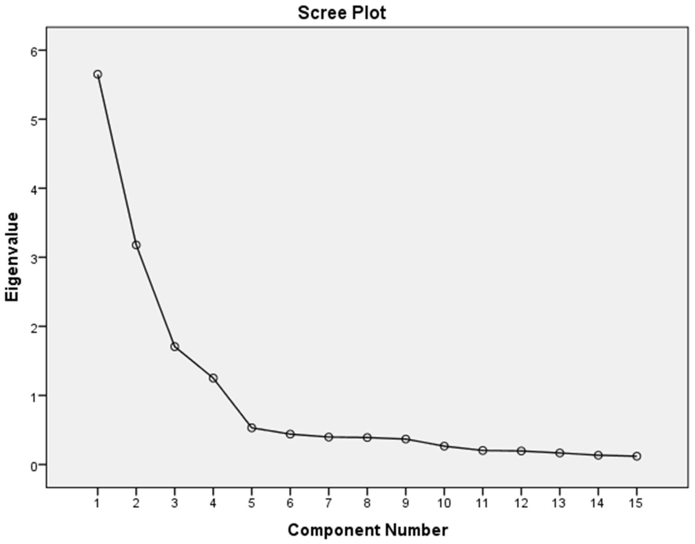Moreover, the Figure 2 of the scree plot also shows that the component number is reliable in further statistical analysis, such as to test the internal consistency of measurement scales.

Measurement Scales of Internal Consistency—Reliability and validity are very important to obtain information on survey questionnaires for individual items respondents have voiced their opinion on [36,47]. However, reliability measures consistency, and validity measures the accuracy of the data [47]. The

Table 4. Internal consistency results of measurement items.

Items	Mean	Corrected Item–Total Correlation	Cronbach’s Alpha (α)		Total N
S1	4.16	0.48	0.90	0.88	302
S2	4.18	0.78	0.83		302
S3	3.85	0.75	0.84		302
S4	4.03	0.78	0.83		302
S5	3.94	0.74	0.84		302
I1	4.25	0.61	0.82	0.84	302
I2	4.23	0.76	0.78		302
I3	4.25	0.71	0.79		302
I4	4.21	0.63	0.82		302
I5	4.24	0.54	0.84		302
EE1	4.01	0.60	0.85	0.86	302
EE2	4.26	0.49	0.88		302
EE3	4.13	0.76	0.81		302
EE4	4.21	0.78	0.80		302
EE5	4.20	0.77	0.81		302
GE1	3.81	0.45	0.83	0.82	302
GE2	4.05	0.66	0.77		302
GE3	4.18	0.74	0.75		302
GE4	4.30	0.67	0.77		302
GE5	4.01	0.59	0.80		302
PSC1	4.22	0.65	0.84	0.86	302
PSC2	4.20	0.79	0.80		302
PSC3	4.24	0.75	0.82		302
PSC4	4.18	0.68	0.83		302
PSC5	4.24	0.54	0.86		302

Source: Empirical data analysis by SPSS [43].

shows the reliability and validity tests executed on the empirical data to obtain their parameters, such as Cronbach’s alpha (α). A value of Cronbach’s alpha (α) ≥0.70 is desirable, while >0.80 is high in social science research [36]. One of the well-known tests for reliability statistics in the procedure method is called Cronbach’s alpha [36,48]. Cronbach’s alpha is a common method to measure reliability when calculating the reliability score to recap the information of numerous items in questionnaires [49].

The Table 4 confirms that the internal consistency of the measurement items achieve more than the desired value of >0.70 [36,48]. The reliability of skills alpha (α) is 0.88, and the validity level is above 0.30, which is good, as the cut-off line of validity is 0.30 [46,50]. However, the alpha value for incentives is 0.84, entrepreneurship education is 0.86, green entrepreneurship is 0.82, and entrepreneurial intention to promote social changes is 0.86, which all demonstrate that the constructs are reliable with the validity scores of the corrected item–total correlation. Indeed, each item of Cronbach’s alpha is reliable and valid. Thus, the variable of each α is >0.70, and the validity of each item is confirmed as >0.30, and thus their parameters are indicated to have strong internal consistency [50]. Therefore, skills, incentives, entrepreneurship education, green entrepreneurship, and entrepreneurial intention to promote social change parameters are confirmed as items that can be demonstrated in empirical survey data for further statistical analysis. Nevertheless, the following section elaborates on the SEM analysis using SmartPLS to validate the structural model to test the hypotheses.

4.2. Structural Equation Model

In the structural equation model, there are two types of analysis. The first analysis is called the partial least square (pls) SEM algorithm, and the second is called the bootstrapping analysis [26,27,28,39,51]. Therefore, the following point is first illustrated by the PLS-SEM algorithm and secondly by the bootstrapping model [39,40,51,52].

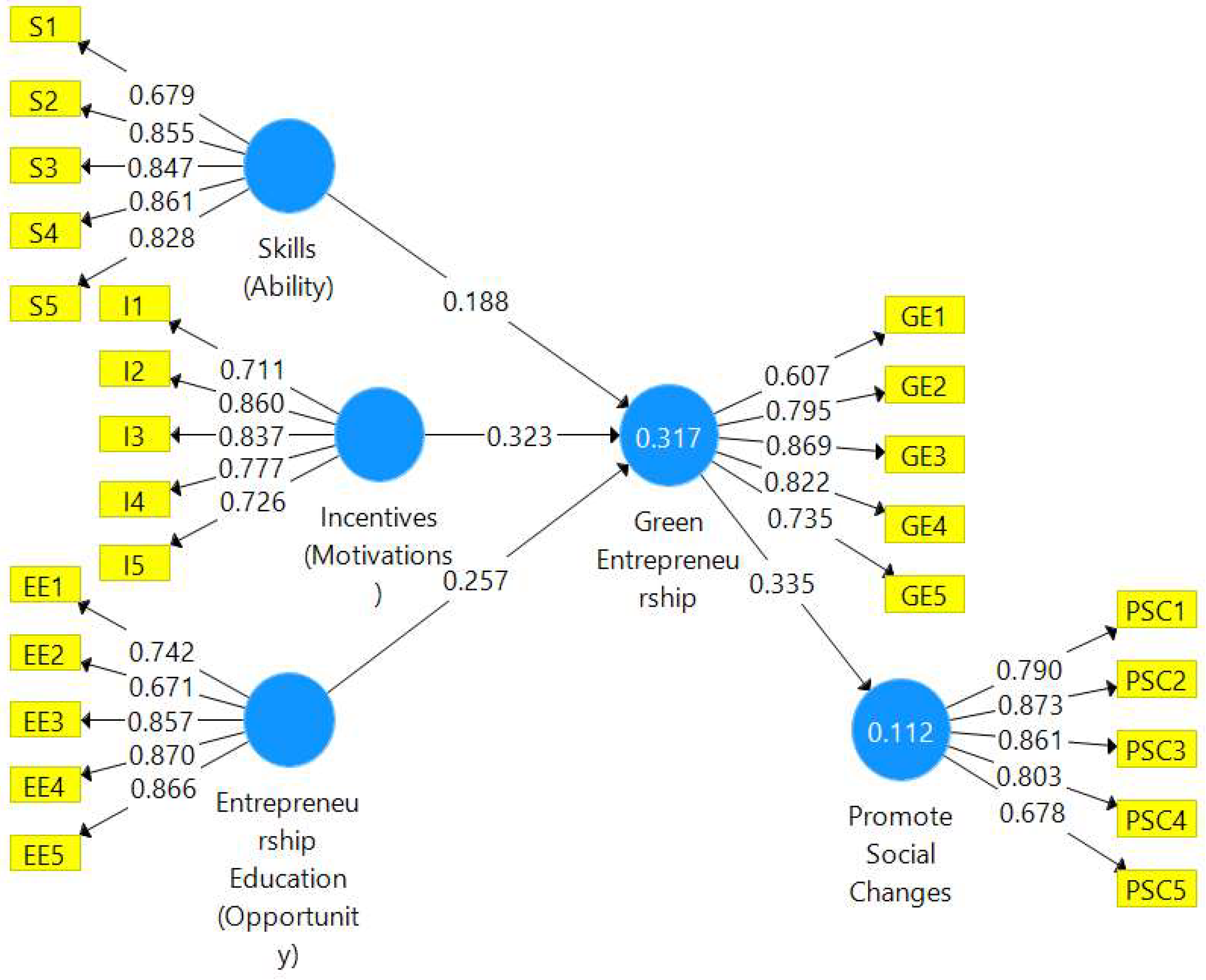
PLS-SEM Algorithm—The Figure 3 of the measuring model is executed by SmartPLS which provides the inter-consistency of survey items for the value of path coefficients (β), outer loadings, construct reliability and validity, discriminant validity, and collinearity statistics. Therefore, the consequent parameters are explained below.

PLS-SEM Algorithm—A number between −1 and +1 is the correlation coefficient [53]. A correlation coefficient greater than 0.6 is sufficient for a student of natural, social, or economic science, whereas correlation coefficients less than 0.3 are regarded as weak, between 0.3 and 0.7 as moderate, and greater than 0.7 as high [53]. From the Figure 3, the path correlations between skills and entrepreneurship education toward green entrepreneurship can be seen to be less than 0.30, i.e., 0.188 and 0.257 with positive but weak relations. Likewise, the correlation between incentives and green entrepreneurship is r = 0.323, which has a moderate and positive relationship. However, the mediating variable of green entrepreneurship and the dependent variable of entrepreneurial intention to promote social change is r = 0.335, which is also a positive and moderate association. Therefore, the path correlation coefficients illustrate that the correlation coefficients are positive between all of them.

Outer Loadings—The outer loadings, for instance, arrows from the latent variable to its indicators, are estimated connections in reflective measurement models [40]. The absolute contribution of an item to its assigned construct is determined by its outside loadings once the loading is ≥0.70 [45]. Though, the range between 0.50 and 0.70 is also acceptable if the HTMT and AVE criterion is reached at the desired value, which is better to assess the discriminant validity [54]. The PLS algorithm demonstrates more than 0.70 for the outer loadings, except for 4 items out of 25. However, the following discriminant validity is checked and no issues are found for Fornell–Larcker or HTMT, despite the cross-loadings of each item. Therefore, the outer loading is estimated as the connection with the latent variables that are demonstrated without any issues and assessed with discriminant validity.

Construct Reliability and Validity—The construct’s reliability and validity is an assessment of the internal consistency for the constructs such as Cronbach’s alpha, rho_A, composite reliability (C.R.), and AVE (average variance extracted) [39,40,45,51,55].

The

Table 5. Construct reliability and validity.

	Cronbach’s α	rho_A	Composite Reliability (C.R.)	Average Variance Extracted
Skills	0.873	0.873	0.909	0.667
Incentives	0.843	0.852	0.888	0.615
Entrepreneurship Education	0.861	0.861	0.901	0.648
Green Entrepreneurship	0.825	0.845	0.878	0.594
Promote Social Changes	0.861	0.873	0.901	0.647

Source: Empirical data analysis by SmartPLS [52].

displays that the phenomenon of Cronbach’s alpha, which measures the internal consistency of the construct, was attained at more than 0.70 with all of the variables [52]. Therefore, each scale item measured the construct closely. On the other hand, the value of rho_A demonstrates whether the value between Cronbach’s alpha and composite reliability is achieved or not [55]. Nevertheless, the rho_A demonstrated in the Table 5 shows that every construct is in between Cronbach’s alpha and composite reliability. Therefore, the value of rho_A perfectly aligns with one of the assessments of internal consistency. Thirdly, the value of composite reliability generated above 0.70 for each construct is similar to Cronbach’s alpha, which is measured by the item for internal consistency. However, C.R. offers a smaller amount of biased calculation than Cronbach’s alpha, provided the construct is reliable and valid. However, the AVE is the mean of the squared loadings of each indicator connected to a build used to compute the AVE [45,52]. Once the average variance extracted (AVE) value is more than 0.50, convergent validity is demonstrated statistically [45,55,56]. However, the Table 5 shows that the AVE is achieved as greater than 0.50. Thus, convergent validity is statistically demonstrated, and there is no issue convergently. Indeed, the assessment for construct reliability and validity is established by every phenomenon.

Discriminant Validity—The level of differentiation and asymmetry between the components is referred to as discriminant validity. According to the rule, variables should have stronger relationships with their factor than with another factor [54]. The

Table 6. Fornell–Larcker criterion.

	Entrepreneurship Education	Green Entrepreneurship	Incentives	Promote Social Changes	Skills
Entrepreneurship Education	0.805
Green Entrepreneurship	0.435	0.771
Incentives	0.193	0.403	0.784
Promoting Social Change	0.413	0.335	0.237	0.804
Skills	0.611	0.397	0.161	0.456	0.817

Source: Empirical data analysis by SmartPLS [52].

displays the first discriminant validity illustrated [52]. It can be seen that entrepreneurship education is more significant than in the column, and green entrepreneurship, incentives, promoting social change, and skills are higher than every column of their engaged row and column.

Fornell–Larcker, cross-loadings, and the outcomes of the HTMT criteria are used to evaluate discriminant validity [54]; however, it is widely recommended to establish discriminant validity using Fornell–Larcker and the HTMT criteria [54]. Likewise, discriminant validity between two reflective conceptions is proven, and if the Fornell–Larcker has a higher value in the same row and column, and the HTMT value is less than 0.90, then discriminant validity is established [39,54]. Therefore, the

Table 7. HTMT criteria.

	Entrepreneurship Education	Green Entrepreneurship	Incentives	Promoting Social Change	Skills
Entrepreneurship Education	0
Green Entrepreneurship	0.507
Incentives	0.219	0.479
Promote Social Changes	0.482	0.393	0.275
Skills	0.710	0.454	0.182	0.521	0

Source: Empirical data analysis by SmartPLS [52].

shows that discriminant validity is established, as every construct is less than 0.90. Therefore, the discriminant validity is established through Fornell–Larcker and HTMT [52].

Collinearity statistics—The variance inflation factor (VIF) is examined to determine the degree of collinearity statistics in PLS-SEM [57,58]. There are two often used guidelines: if the VIF value is 5 or greater, there may be a collinearity problem [54]. Indeed, in the measurement items, there are no values which are less than 4. However, the VIF values are mostly less than 3. Therefore, no collinearity issues in the measured items are found, and all of the PLS algorithms have provided outputs that are desirable. Thus, we can continue to the path analysis for the hypotheses test predicted by the literature with the deductive approach.

4.3. Bootstrapping of the Path Model

With the path model, it is possible to assess the statistical significance of different PLS-SEM outcomes, such as path coefficients and r-square (R²) values, using the nonparametric approach of bootstrapping [51,54]. Consequently, the following bootstrapping model and results are clarified.

Path Coefficients—Path coefficients are normalized versions of linear regression weights that may be employed in the structural equation modeling technique to investigate potential causal relationships between statistical data [51].

The

Table 8. Path coefficients.

	Correlations	T Statistics	p Values	Remark
Skills -> Green Entrepreneurship	0.187	2.863	0.004	H1 accepted
Incentives -> Green Entrepreneurship	0.324	5.240	0.000	H2 accepted
Entrepreneurship Education -> Green Entrepreneurship	0.257	3.529	0.000	H3 accepted
Green Entrepreneurship -> Promoting Social Change	0.335	2.978	0.003	H4 accepted

Source: Empirical data analysis by SmartPLS [52].

confirms the two most common components, t-statistics and the p-values, are achieved by the cut-off value [52]. However, if the t-statistic is 1.96, then it becomes significant when the p-value is ≤0.05 [40,45,50,55,59]. The path direction of hypothesis, H1, is accepted for skills → green entrepreneurship: the t-statistic is 2.863 and the p-value is 0.004, which is ≥1.96 for the t-statistic, and ≤0.05 for the p-value. Therefore, hypothesis H1 is established by the literature and is confirmed as statistically significant. The factor of skills is strongly associated with green entrepreneurship. Thus, if students have the opportunity to develop their skills at university level then the business will be aligned with the green concept that is demonstrated in emerging nations such as Bangladesh [3,9,10,18]. The second hypothesis, H2, of incentive → green entrepreneurship is illustrated at the desired level: the t-statistic is 5.24 and the p-value is 0.000, which is greater than 1.96 and less than 0.05, respectively. Therefore, in this scenario, the student is motivated to start the business and also has a positive significant association with green entrepreneurship. Thus, incentive has more power to motivate university students to think green [3,18,20]. Likewise, if we look at the third hypothesis, H3, the relationship of entrepreneurship education → green entrepreneurship is also strongly related: the t-statistic is 3.529 and the probability level is 0.000. Therefore, hypothesis H3 achieved more than 1.96 and a p-value smaller than 0.05, which means that proper guidance and practical learning have a strong relationship. Moreover, opportunity allows students with a positive mindset embrace a green approach [18,32]. Nevertheless, the final hypothesis is also confirmed by the empirical data: the t-statistic is 2.978 and the p-value is 0.003. 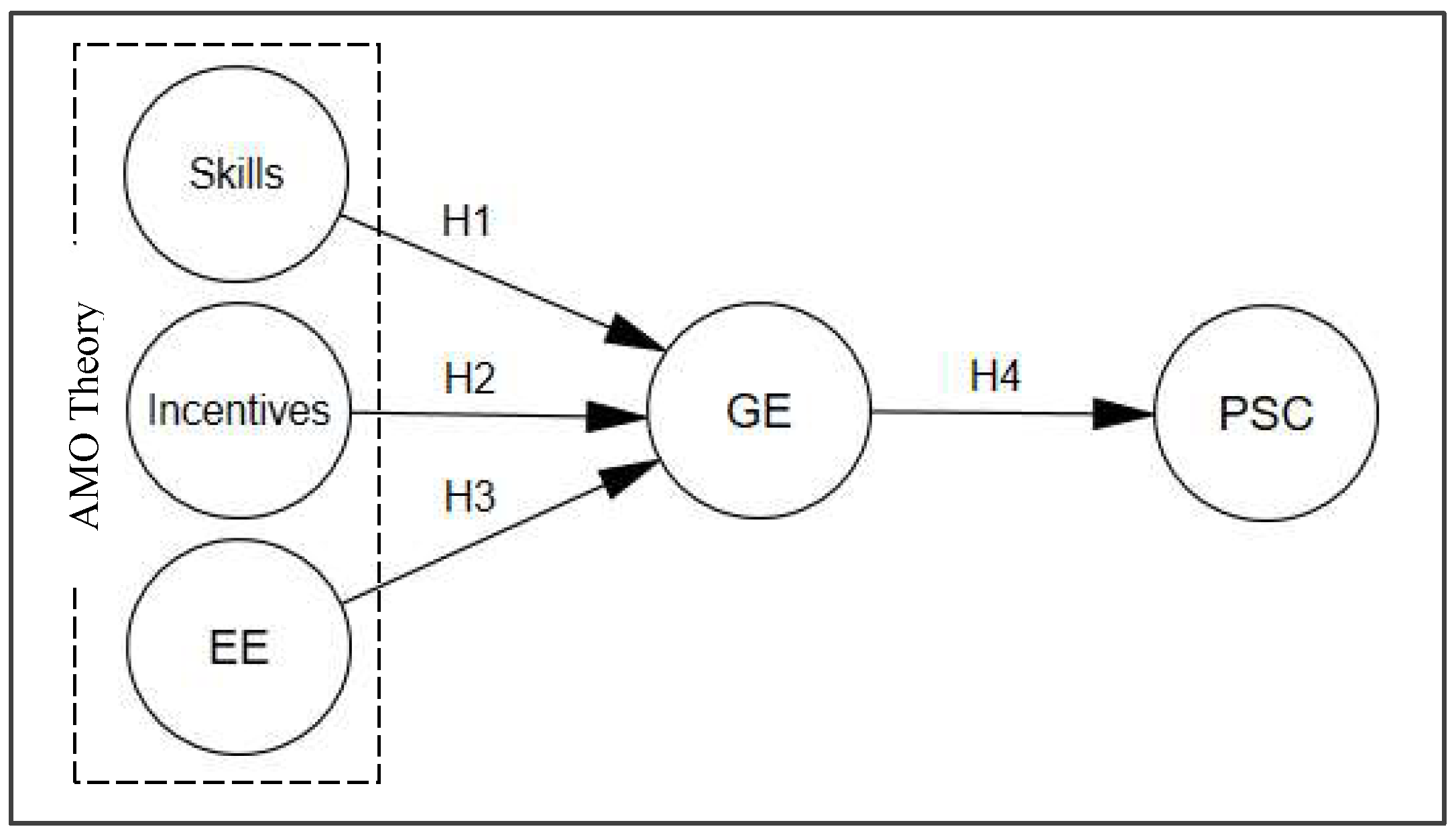Therefore, hypothesis H4 is accepted, confirming the significant relationship (Figure 1). An entrepreneurship education encourages businesses to think green by installing solar panels, employing eco-friendly businesses, and undertaking recycling operations. Many prospective businesses can be considered green enterprises by embracing creative opportunists and ethical views [6,18,20]. Indeed, the four hypotheses are demonstrated to be statistically significant by the survey data, in which respondents offered their opinion on a Likert scale of 1 to 5 points.

The

Table 9. Specific indirect effects.

	Original Sample	T Statistics	p Values	Remark
Skills -> Green Entrepreneurship -> Promoting Social Change	0.06	1.90	0.058	Closely significant mediation.
Incentives -> Green Entrepreneurship -> Promoting Social Change	0.11	2.22	0.027	Mediation demonstrated.
Entrepreneurship Education -> Green Entrepreneurship -> Promoting Social Change	0.09	2.14	0.033	Mediation demonstrated.

Source: Empirical data analysis by SmartPLS [52].

displays the specific indirect effects of mediation between skills and promoting social change with green entrepreneurship, which are closely related. However, the t-statistic is 1.90 and the p-value is 0.058; thus, the cut-off line of the t-value should be 1.96, and the p-value becomes 0.05 [40,45,50,55,59]. Therefore, the mediation of skills and promoting social change through green entrepreneurship have a poorly fit indirect relationship. On the second mediation between incentives and promoting social change, a statistically significant relationship is demonstrated through green entrepreneurship. The value of the t-statistic is 2.22 and the p-value is 0.27, which is more than 1.96, and the p-value is achieved at less than 0.05. Eventually, the mediation between entrepreneurship education and promoting social change through green entrepreneurship achieved a significant and positive association. The t-statistic is 2.14 and the p-value is 0.033, which is greater than the cut-off line of the t-value with a statistically identified p-value as well. Therefore, the conceptual model demonstrates hypothetical and statistical significance with direct and partial mediation as well, and the four hypotheses are positively significant with mediation.

R² (r-square)—The values of R² vary from 0 to 1, and they are frequently expressed as percentages from 0% to 100% [39,55]. Therefore, the R² of 100% indicates that changes in the independent variable fully explain all changes in another dependent variable. However, from the Figure 4 displays that the value of R² is 0.317 for green entrepreneurship, which is around 32% of that predicted by the variables of skills, incentives, and entrepreneurship education [60,61,62]. Entrepreneurial intention to promote social change is 0.112, which is 11% influenced by green entrepreneurship. Therefore, the rest of the influence might be other predictable variables. However, the dependent variable was influenced poorly at only 11% by green entrepreneurship, whereas 89% (100–11) might be other predicted variables. Therefore, the research hypotheses demonstrate that the research model is valid and it will be helpful for students to adopt a green mindset instead of traditional propensity.

5. Discussion

Our research objective was to explore and enhance a structural model influenced by AMO theory of deductive approaches from the perspective of university students and their entrepreneurial intention to go green. The validation of the model was conducted with SmartPLS to explore the prediction enhancement. The components were identified with 5 constructs and a total of 25 measured items, which were statistically significant and validated by the empirical literature review. The model was identified as statistically significant, which was predicted earlier in this study with hypothesis association. AMO theory has influenced and connected green entrepreneurship towards intention enhancement, the promotion of social change, and adopting green business sustainability through structural equation modeling (SEM) analysis. Four hypotheses are developed in the current study in comparison with past empirical literature. Therefore, exploratory analysis supported the survey data that were chosen for the research method earlier in this study. However, the literature and the students’ perceptions positively influenced the factors of AMO theory towards green entrepreneurship, and entrepreneurial intention promoted social change with sustainability for business development. Eventually, skills, incentives, and entrepreneurship education were positively associated with green entrepreneurship intention to become a positive entrepreneur at university level. This can be achieved by taking entrepreneurship education courses. Businesses should be environmentally friendly and ensure a green economy for emerging future nations. Green entrepreneurs are viewed as leading change-makers who can bring about societal changes in the areas of environment, society, and ethics [2,3,9].

Likewise, Figure 5 shows that the highest response was related to incentive, which is demonstrated as the most important factor for green entrepreneurship among the factors of AMO theory. The second highest factor was entrepreneurship education and the students’ perceptions. Indeed, AMO theory is demonstrated by its three statistically significant and positive path coefficients towards green entrepreneurship that are influenced by the entrepreneur’s intention for social change.

There is a limitation to this research: data were collected only from respondents with business studies backgrounds. However, further research needs to view students’ perceptions of different backgrounds to identify measurement scales. Therefore, further study may suggest that survey data from students of different backgrounds may give more diverse intentions to justify entrepreneurship and entrepreneurial intention measurement items. However, by enhancing students’ skills, incentives, and entrepreneurship education through green entrepreneurship effective performance, and chances for knowledge-sharing and problem-solving involvement [1], this research model enables the entrepreneur to promote social change to a high-performing class. Eventually, this study can help researchers to research structural equation modeling (SEM) to develop this model with different factors, or to test the theory for confirmation with a covariance-based SEM model rather than a variance-based SEM model.