
Revisiting the Mousetraps Experiment: Not Just about Nuclear Chain Reactions


1
Consorzio Interuniversitario Nazionale per la Scienza e la Tecnologia dei Materiali (INSTM), 50121 Florence, Italy
2
Dipartimento di Chimica, Università degli Studi di Firenze, Via della Lastruccia 3, 50019 Sesto Fiorentino, Italy
*
Author to whom correspondence should be addressed.
Systems 2022, 10(4), 91; https://doi.org/10.3390/systems10040091
Submission received: 13 May 2022
/
Revised: 27 June 2022
/
Accepted: 28 June 2022
/
Published: 29 June 2022
(This article belongs to the Section Complex Systems)
Abstract
:We present here the first quantitative measurements of a classic experiment, that of the “mousetrap chain reaction”. It was proposed for the first time in 1947 to illustrate the chain reaction occurring in nuclear fission. It involves several spring-loaded mousetraps loaded with solid balls. Once one trap is made to snap, it releases two balls that may trigger the other traps. The result is a chain reaction that rapidly flares and then subsides as most traps have been triggered. The experiment has been popular as a scientific demonstration, but it does not seem that quantitative data were ever reported about it, nor that it was described using a model. We set out to do exactly that, and we can report for the first time that the mousetrap experiment can be fitted by a simple dynamic model derived from the well-known Lotka-Volterra one. We also discuss the significance of this experiment beyond nuclear chain reactions, providing insight into a variety of fields (chemistry, biology, memetic, natural resources exploitation) involving complex adaptive systems.
1. Introduction
The “mousetrap experiment” was proposed in 1947 by Richard Sutton [1] as a mechanical simulation of the chain reaction that occurs in fissile nuclei, such as the 235 isotope of Uranium. This self-amplifying chain is characterized by a “positive feedback” (amplification), which is a peculiarity of nonlinear complex systems [2]. The mousetrap experiment is aimed at visualizing such a complexity. It consists of loading several (typically 50–100) spring-loaded mousetraps with solid balls fitted to the metal bar. Triggering one of the traps results in a chain reaction with the release in the air of two balls, which may then land on other traps, leading to the release of more balls. The result is a rapid explosion of flying balls that subsides when most of the traps have been triggered. The trap simulates a uranium nucleus, while the balls simulate the neutrons that trigger fission in other nuclei.
Today, tens, perhaps hundreds, of videos of examples of the mousetrap experiment can be found over the Web. But it does not appear that anyone ever quantified the parameters of the reaction or tried to reproduce it by a mathematical model. This is what we set out to perform by measurements and through a simple system dynamic model, the “Single-Cycle Lotka-Volterra” (SCLV) model that we developed in earlier papers to describe the phenomenon of overexploitation in economic systems [3,4]. We found that the model can describe the dynamics of the mousetrap experiment. We believe that this approach adds interest to an experiment that has great value for the dissemination of dynamic concepts not just in nuclear physics, but also in fields such as ecology, economics, and memetics.
2. Materials and Methods
We examined several available sets of data for the mousetrap experiment. One source of data was video clips found on the Web; another set was obtained from an experimental set-up created by the authors. We found only a few experiments on the Web where the experimental data could be quantified. In most cases, the traps were not fixed to the supporting plate, so the result was that the balls and traps flew in the air together and triggered other mousetraps during the chain reaction. This is probably performed to obtain a more spectacular result, but the experiment becomes different from what it is supposed to be. Nevertheless, we found experiments on the Web where the traps were fixed to the plate that held them [5,6].
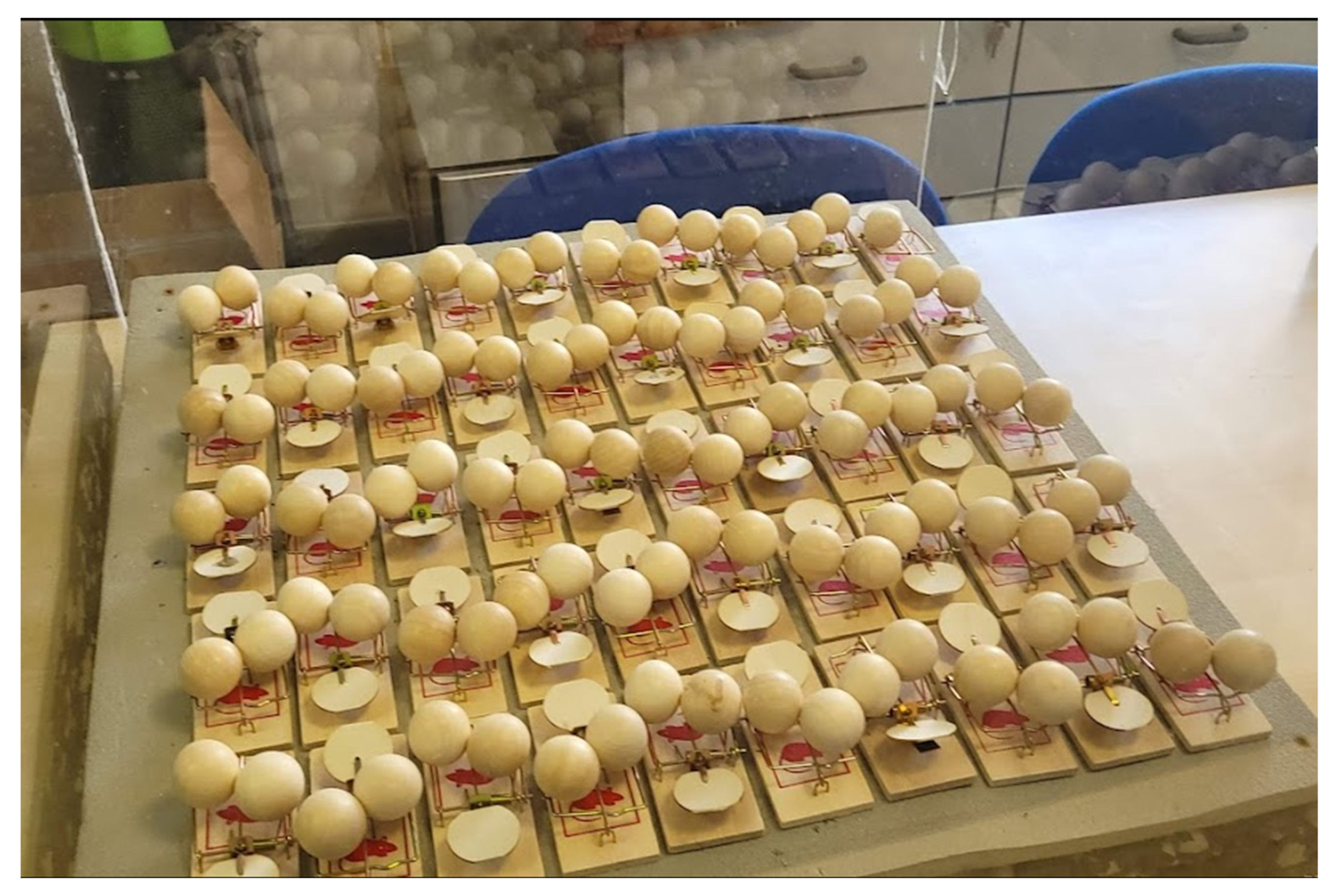
The author’s experimental set-up was built in Florence using 50 commercial mousetraps, each of 50 × 95 mm (Figure 1). The traps were set on five rows of 10 traps each, spaced about 5 mm from each other, and covering a square of 55 × 55 cm. They were glued to a soft plastic underlying material to avoid vibrations that could cause the traps to trigger each other. The square was enclosed in a cubic transparent plexiglass enclosure of 62 cm × 62 cm. Each trap was loaded with two wooden balls of 30 mm in diameter. The sensitivity of the triggering mechanism was enhanced by fixing 25-mm rigid cardboard disks to the original metal trigger. In these conditions, we found that the chain reaction was completed in ca. 2–3 s, leaving just a few traps still loaded with balls. As reported by other authors [7], setting the traps requires a certain manual dexterity that the authors of this paper acquired by trial and error, suffering only minor damage to their fingers in the process.
In all cases, we determined the parameters of the chain reaction using video recordings run in slow-motion to count the flying balls and the triggered traps. For the Florence experiment, we used the cameras of commercial Samsung cell phones used in slow motion at ½ or ¼ of the real speed. For the Web experiments, we used the video clips available. In all cases, we used the site www.watchframebyframe.com (accessed on 12 May 2022) to count the flying balls as a function of fixed intervals of time.
Counting the balls in this way involved a certain degree of uncertainty related to detecting moving balls close to the traps and to reflections of the balls on the plexiglass walls enclosing the experimental volume. Nevertheless, repeated tests on the same experiments showed that the uncertainty was at most one or two balls, and it did not prevent the determination of the kinetics of the experiment.
3. Results
3.1. The Berkeley Experiment
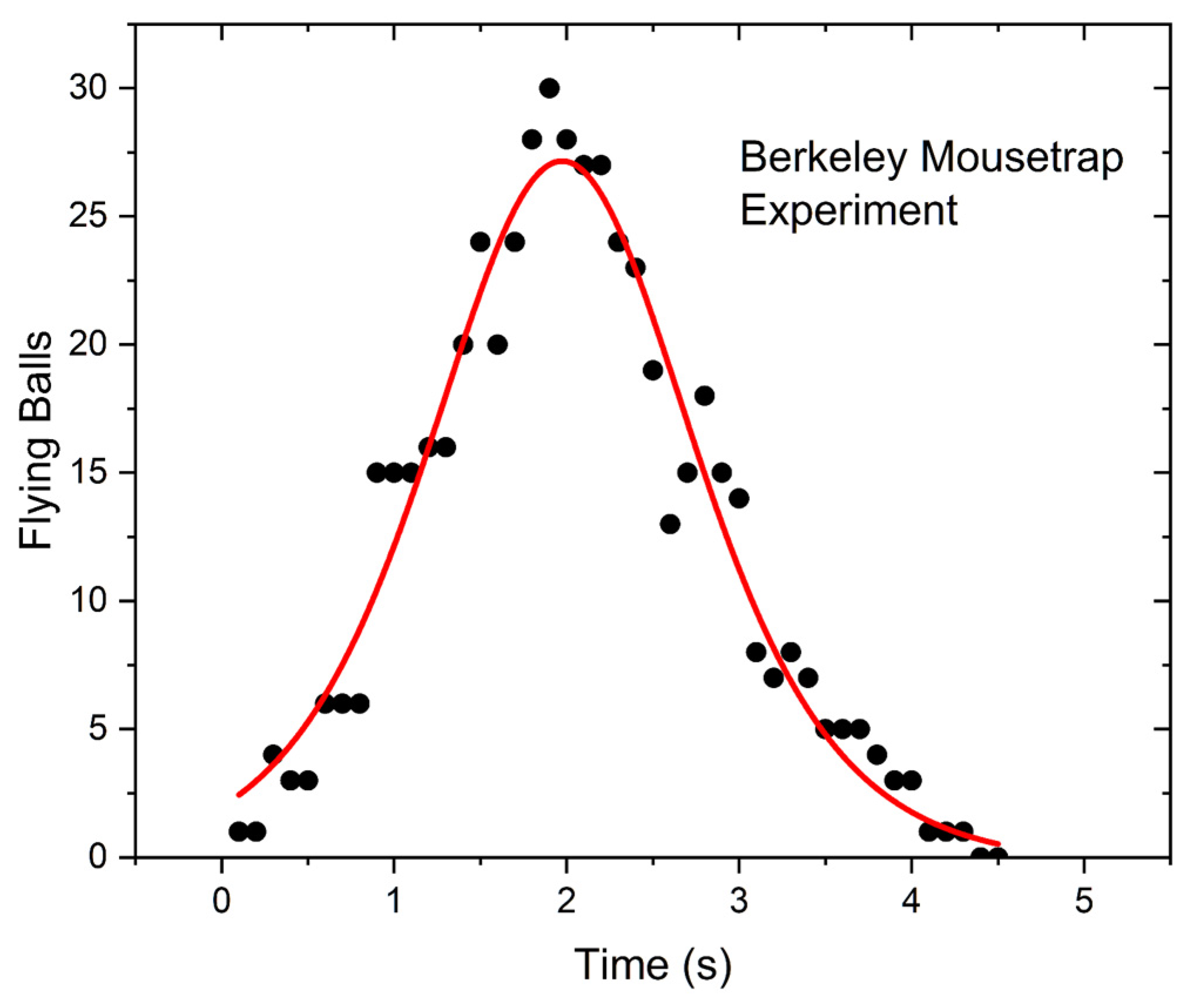
This test involved 49 mousetraps, each one loaded with two plastic balls (“superballs”). Unlike most set-ups of this experiment, the traps were not triggered by a mechanical trigger, but by a solenoid connected to a metal strip acting as a spring. The chain reaction lasted about 4 s. From the video, it was possible to count the flying balls but not the number of triggered traps as a function of time. The results are shown in Figure 2. The experimental points were fitted with the derivative of a logistic function. Note the “bell-shaped” form of the curve.
3.2. The Dalton Nuclear Experiment
In the description, the experiment is said to have involved 200 traps loaded with one ball each. The images, however, showed that only 110 traps (and as many balls) were used. The experiment was shown in slow motion, and the chain reaction shown lasted for 90 s. Unfortunately, the authors did not report the motion rate they used. Assuming that each frame corresponds to 0.25 s, the whole reaction may have lasted around 3 s. Although the time scale is uncertain, the shape of the curve for the flying balls was, again, “bell-shaped”. The results are shown in Figure 3. In this case, it was not possible to detect the number of triggered traps as a function of time.
3.3. The Florence Experiment
In the previous two experiments (Berkeley and Dalton), it was only possible to keep track of the flying balls, not of the triggered traps. Our experimental set-up was designed to provide these missing data. We used two cameras, one recording from above, the other from one side. In this way, it was possible to count both the flying balls and the triggered traps. Typical results for a single run are shown in Figure 4. Here, for illustrative purposes, the number of flying balls was fitted with the derivative of a logistic, while the number of untriggered traps was fitted with a simple logistic decay.
These experiments were well repeatable with the same setup, even though, as would be expected, the results of the measurements varied depending on random factors associated with the limited number of traps. In all the tests, we found that the number of flying balls followed a bell-shaped curve, while the number of untriggered traps declined according to a logistic curve.
3.4. The Mousetrap Mathematical Model
A logistic curve and its derivative provide a first understanding of a typical phenomenon of growth and stabilization in complex systems, such as in chemistry and biology. We observed that, indeed, the logistic provided a good fitting with the experimental data in all the three mousetrap experiments examined here. Nevertheless, the logistic function did not provide a direct link to the physical properties of the system. For this purpose, we developed a mechanistic model that directly describes the experimental parameters using the methods of system dynamics.
We started from the observation that the system has a thermodynamic component: the potential energy stored in the springs of the mousetraps tends to be dissipated when the trap snaps. Balls are the catalyst that makes it possible for this energy to be released. It is accumulated for a short time as the kinetic energy of the flying balls and is finally dispersed as high entropy thermal energy. This kind of phenomenon is common in biology; it describes a trophic chain, where an initial stock of metabolic energy is dissipated in steps by a series of predator–prey relationships. The simplest model that describes trophic chains is the well-known Lotka-Volterra (LV) model [8].
For the Florence experiment, we used a modification of the LV model that we call the “Single-Cycle Lotka Volterra” (SCLV) to take into account that the traps are not recharged (do not “reproduce”) during the experiment. We developed this model in previous studies [9] to describe socio-economic systems that exploit non-renewable or slowly renewable resources [3,10]. The SCLV model used the same equations as the LV model, but the term that describes the growth of the prey population was set to zero. It is described by two coupled differential equations:
where “L1” (“Level 1) stands for the potential energy stored in the traps. It is measured using the number of cocked traps as a proxy. “L2” (“Level 2”) is the kinetic energy stored in the flying balls, measured in terms of the number of balls in the air. The ks are constants whose value depends on the unit of measurement of the levels.
dL1/dt = −k1L1L2
dL2/dt = k2L1L2 − k3L2
The first equation of the model assumes that the number of traps snapping per unit time is proportional to both the number of flying balls and the number of untriggered traps. Of course, when either one of these parameters is zero, the reaction does not take place. The second equation describes the number of flying balls, also proportional to the number of flying balls and the number of cocked traps. Finally, the second term of the second equation describes the loss of energy of the flying balls as they come to rest on the table.
The model was tested using a standard fitting procedure implemented in MATLAB (the unconstrained nonlinear optimization method based on the Nelder-Mead algorithm, termed “fminsearch”). The data examined were only those of the Florence experiment, since, as described before, it was not possible to have complete data for the other two experiments. The measurements for the flying balls were averaged and linearly interpolated when they had been taken at a different frame rate. As a result, the points do not correspond to integers. The results are shown in Figure 5.
The fitting was initialized with the number of traps set at 50 and the flying balls at 1. The initial values of k1, k2, and k3 were roughly estimated by considering an exponential decay of the triggered traps (k1); exponential growth of the flying balls when the reaction chains start (k2); and an exponential decline of the number of flying balls when traps are almost at the minimum (k3). Once initialized, the fitting returns with the constant values in Figure 5.
The fitting led to an initial number of flying balls equal to 0.6, a reasonable approximation of the fact that the chain reaction started with a single ball. Note that k1 and k2 are expressed in N−1 s−1 units, with N = number of balls. k3 is expressed in s−1. Remarkably, the fitting converged by itself to a ratio of k2/k1 nearly equal to 2, which is what would be expected since every ball that triggers a trap releases two balls. This ratio corresponds to the “reproduction rate” in biological populations. Other experimental runs provided similar results, although in some cases the ratio was slightly higher than 2. It may have been the result of a ball triggering more than a single trap or just of fluctuations in the data.
The numerical coefficients can be used to determine the “net reproduction rate” according to the common definition in population biology. It is the number of new individuals (flying balls) divided by the number of deaths (balls on the ground). In the mousetrap experiment, this parameter is given by the new flying balls k2L1L2 generated per unit time divided by the fallen balls for the same unit time, that is k3L2. The result is (k2/k3)L1. At t = 0 (50 untriggered traps), this number is 1.8, close to 2, as one would expect. For t > 0, the net reproduction rate falls and becomes smaller than one when the population of flying balls does not grow anymore. In this specific run, it occurs at the peak of the flying ball population, for L1 = 28 untriggered traps. The final value of the net reproduction rate is 0.43 for 12 untriggered traps, when there are no more flying balls.
We can also use these values to estimate the “critical mass” of the trap system. For L1 < 25, the net reproduction rate is smaller than one and the system should not show a chain reaction. We verified this result experimentally, finding that, indeed, for less than 25 traps loaded with balls, the chain reaction either does not start or it involves only 2–3 traps before stopping. Note that no experimental setup shown on the Web appears to use less than 25 traps. This lower limit was found by other authors by trial and error.
4. Discussion
The mousetrap experiment was developed during the period called “the atomic age,” in the late 1940s [1], as a tool for explaining to the public the mechanism of the chain reaction in nuclear explosions. The mousetrap experiment was supposed to be noisy and spectacular, and it succeeded in attracting much attention. It even appeared in a popular Walt Disney movie, “Our Friend, the Atom” in 1957.
Of course, this experiment is very limited as a simulation of a nuclear explosion; the number of traps that can be reasonably used is much smaller than the number of nuclei involved in a real atomic chain reaction. In addition, in the real world, there does not exist a neutron reflector with properties comparable to the glass box used to contain the balls, but, overall, the experiment does describe the main feature of a chain reaction: the effect we call today “enhancing” or “positive” feedback [11].
Using a controlled experimental set-up and well-known system dynamics methods, we found that the experiment can be modeled, and the model can be used to extract the fundamental parameters of the system, such as the “net reproduction rate” and the “critical mass” of the mousetrap array. To our knowledge, this determination was never carried out in previous tests with this set-up.
Our idea in re-examining this old experiment was not to add details to something already well-known. It was to show how general the phenomenon of energy transfer in trophic chains is, to the point that it can be simulated by mechanical devices. The first result was to demonstrate how the SCLV model can simulate the mousetrap experiment. We concluded that it can be considered as a general model for this kind of system, as we argued in a previous paper [9].
The mousetrap array system can also be described in terms of network theory. In this case, each trap forms a node of the network, while the flying balls provide connections between nodes. Each trap is reachable by a flying ball in times much smaller than the overall chain reaction cycle, so that the network can be classified as a “fully connected” one. A larger mousetrap network would behave differently: the chain reaction would show a spatially advancing wave moving along the trap array. In this case, however, the “fully connected” network condition is closer to that of the originally modeled system, a nuclear chain reaction, where all the nuclei in the system are equally reachable by free neutrons. This kind of network react to external stimuli by amplifying the initial perturbation.
The first ball dropped on the mousetrap array can be seen as a packet of energy, a signal that is picked up by one of the mousetraps. The network then amplifies the signal, in this specific system, by about a factor of 10. That is, starting from one ball, there is a moment during the reaction when 10 balls are flying. In this sense, the system behaves like an electron multiplier of the kind used in night-vision systems. In that case, though, the gain may go from 105 to 108 and more.
Examples of this enhanced feedback behavior can be easily found in ecosystems. For instance, the balls can be seen as pathogens and the traps as susceptible people. In this case, the model can describe the flaring of an epidemic in a susceptible population according to the “SIR” (susceptible, infected, removed) model [12]. It is well known that epidemics tend to flare and then subside when “herd immunity” is reached. More complex ecosystems tend to be stable, and Makarieva et al. [13] discussed the difference between inorganic systems such as tornadoes and biological systems, noting how tornadoes flare up and rapidly subside, unlike ecosystems. They attributed the stability of ecosystems to the control of the genome of the living system on the environment, a concept termed “biotic regulation” [14]. In addition to this concept, it may be that part of the difference is because tornadoes are local phenomena understandable as fully connected, such as the mousetrap array. Ecosystems, instead, are in large part based on local interaction and the signal moves slowly throughout the system, so that explosive flaring is not observed.
Economic systems often behave as biological systems; for instance, if the ball is seen as a stock of exergy, then the traps can be seen as oil wells, and the chain reaction involves re-investing part of this energy into exploiting new fossil resources. The “production” curve, in this case, is the well-known “Hubbert curve” [15]. In general, if the balls are seen as non-renewable or slowly renewable resources, the chain reaction describes the phenomenon of overexploitation. We observed this behavior also in fisheries [4,10]. On this point, the “net reproduction rate” in the previous section corresponds to the “Rt” rate in epidemiology and to the EROEI, or EROI (energy return for energy invested) [16], for several energy production systems that exploit non-renewable resources, e.g., oil, as we noted in a previous study [17].
We may also see the mousetrap experiment as a model for the World Wide Web. In this case, the signal takes the name of “meme”, and the resulting diffusion over the web is termed “going viral.” In a previous paper, Bardi et al. showed that the LV model could describe the diffusion of memes on the Web [18].
Mousetraps seem to be the only simple mechanical device that can be bought at a hardware store that can be used to create a chain reaction. We do not know why this phenomenon is so rare in hardware stores, but chain reactions are surely common in complex adaptive systems. We believe that the results we reported in this paper can be helpful to understanding such systems and, if nothing else, to illustrate how chain reactions can easily go out of control, not only in a critical mass of fissile uranium but also in similar dynamics occurring in the ecosystem that go under the name of “overshoot” and “overexploitation”.
Author Contributions
Conceptualization, U.B.; methodology, I.P.; software, I.P.; validation, U.B. and I.P.; formal analysis, U.B.; investigation, I.P.; resources, U.B.; data curation, U.B.; writing—original draft preparation, U.B.; writing—review and editing, I.P.; visualization, I.P.; supervision, U.B. All authors have read and agreed to the published version of the manuscript.
Funding
This research received no external funding.
Institutional Review Board Statement
Not applicable.
Informed Consent Statement
Not applicable.
Data Availability Statement
Not applicable.
Acknowledgments
The authors thank James Little, the author of the Berkeley mousetrap experiment, and the authors of the Dalton Nuclear mousetrap experiments.
Conflicts of Interest
The authors declare no conflict of interest.
References
- Sutton, R.M. A Mousetrap Atomic Bomb. Am. J. Phys. 1947, 15, 427–428. [Google Scholar] [CrossRef]
- Forrester, J.W. Urban Dynamics; Pegasus Communications: Boston, MA, USA, 1968. [Google Scholar]
- Perissi, I.; Bardi, U.; El Asmar, T.; Lavacchi, A. Dynamic patterns of overexploitation in fisheries. Ecol. Model. 2017, 359, 285–292. [Google Scholar] [CrossRef]
- Bardi, U.; Lavacchi, A. A Simple Interpretation of Hubbert’s Model of Resource Exploitation. Energies 2009, 2, 646–661. [Google Scholar] [CrossRef]
- Little, J. Mousetrap Chain Reaction Experiment. Physics Berkeley. Available online: http://berkeleyphysicsdemos.net/node/708 (accessed on 12 May 2022).
- A Chain Reaction (with Mousetraps and Ping Pong Balls). Dalton Nuclear. Available online: https://www.youtube.com/watch?v=9e8E0T8hfco (accessed on 12 May 2022).
- Higbie, J. The better mousetrap: A nuclear chain reaction demonstration. Am. J. Phys. 1980, 48, 86–87. [Google Scholar] [CrossRef]
- Tyutyunov, Y.V.; Titova, L. From lotka–volterra to Arditi–Ginzburg: 90 years of evolving trophic functions. Biol. Bull. Rev. 2020, 10, 167–185. [Google Scholar] [CrossRef]
- Perissi, I.; Lavacchi, A.; Bardi, U. The Role of Energy Return on Energy Invested (EROEI) in Complex Adaptive Systems. Energies 2021, 14, 8411. [Google Scholar] [CrossRef]
- Perissi, I.; Bardi, U. The future: The blue economy. In The Empty Sea; Springer: Cham, Switzerland, 2021; pp. 129–173. [Google Scholar] [CrossRef]
- Richardson, G.P. System dynamics. In Encyclopedia of Operations Research and Management Science; Kluwer Academic Publishers: Boston, MA, USA, 1996; pp. 1519–1522. [Google Scholar] [CrossRef]
- Kermack, W.O.; McKendrick, A.G. Contributions to the mathematical theory of epidemics. II.—The problem of endemicity. In Proceedings of the Royal Society of London. Series A, Containing Papers of a Mathematical and Physical Character; Royal Society Publishing: London, UK, 1932; Volume 138, pp. 55–83. [Google Scholar]
- Makarieva, A.M.; Nefiodov, A.V.; Li, B.-L. Life’s Energy and Information: Contrasting Evolution of Volume- versus Surface-Specific Rates of Energy Consumption. Entropy 2020, 22, 1025. [Google Scholar] [CrossRef]
- Gorshkov, V.; Makarieva, A.M.; Gorshkov, V.V. Biotic Regulation of the Environment: Key Issues of Global Change; Springer Science & Business Media: London, UK, 2000. [Google Scholar]
- Hubbert, M. Nuclear Energy and the Fossil Fuels. In Proceedings of the Spring Meeting of the Southern District, American Petroleum Institute, Plaza Hotel, San Antonio, TX, USA, 7–9 March 1956. [Google Scholar]
- Hall, C.A.; Lambert, J.G.; Balogh, S.B. EROI of different fuels and the implications for society. Energy Policy 2014, 64, 141–152. [Google Scholar] [CrossRef] [Green Version]
- Bardi, U.; Lavacchi, A.; Yaxley, L. Modelling EROEI and net energy in the exploitation of non renewable resources. Ecol. Model. 2011, 223, 54–58. [Google Scholar] [CrossRef]
- Perissi, I.; Falsini, S.; Bardi, U. Mechanisms of meme propagation in the mediasphere: A system dynamics model. Kybernetes 2019, 48, 79–90. [Google Scholar] [CrossRef]
Figure 1.
The Florence mousetrap experiment.

Figure 2.
The results of the Berkeley mousetrap experiment (4).

Figure 3.
The Dalton nuclear experiment [6].
Figure 3.
The Dalton nuclear experiment [6].

Figure 4.
Typical results of the Florence experiments. This figure shows an average of three tests. The data were fitted with a simple logistic equation (upper curve) and the derivative of a logistic equation (lower curve).
Figure 4.
Typical results of the Florence experiments. This figure shows an average of three tests. The data were fitted with a simple logistic equation (upper curve) and the derivative of a logistic equation (lower curve).

Figure 5.
Results of the fitting of the data for the Florence experiment using the SCLV model. The Y scale is the number of balls/untriggered traps. The coefficients for this specific fitting were found to be k1 = 0.0604, k2 = 0.1212, k3 = 3.3092.
Figure 5.
Results of the fitting of the data for the Florence experiment using the SCLV model. The Y scale is the number of balls/untriggered traps. The coefficients for this specific fitting were found to be k1 = 0.0604, k2 = 0.1212, k3 = 3.3092.

Publisher’s Note: MDPI stays neutral with regard to jurisdictional claims in published maps and institutional affiliations. |
© 2022 by the authors. Licensee MDPI, Basel, Switzerland. This article is an open access article distributed under the terms and conditions of the Creative Commons Attribution (CC BY) license (https://creativecommons.org/licenses/by/4.0/).
Share and Cite
MDPI and ACS Style
Perissi, I.; Bardi, U. Revisiting the Mousetraps Experiment: Not Just about Nuclear Chain Reactions. Systems 2022, 10, 91. https://doi.org/10.3390/systems10040091
AMA Style
Perissi I, Bardi U. Revisiting the Mousetraps Experiment: Not Just about Nuclear Chain Reactions. Systems. 2022; 10(4):91. https://doi.org/10.3390/systems10040091
Chicago/Turabian StylePerissi, Ilaria, and Ugo Bardi. 2022. "Revisiting the Mousetraps Experiment: Not Just about Nuclear Chain Reactions" Systems 10, no. 4: 91. https://doi.org/10.3390/systems10040091
Note that from the first issue of 2016, this journal uses article numbers instead of page numbers. See further details here.