
Stock Price Crash Warning in the Chinese Security Market Using a Machine Learning-Based Method and Financial Indicators


1
College of Economics and Management, China Three Gorges University, Da Xue Road No.8, Yichang 443002, China
2
School of History, Beijing Normal University, Beijing 100875, China
*
Author to whom correspondence should be addressed.
Systems 2022, 10(4), 108; https://doi.org/10.3390/systems10040108
Submission received: 3 May 2022
/
Revised: 8 July 2022
/
Accepted: 25 July 2022
/
Published: 29 July 2022
(This article belongs to the Special Issue Decision-Making Process and Its Application to Business Analytic)
Abstract
:Stock price crashes have occurred frequently in the Chinese security market during the last three decades. They have not only caused substantial economic losses to market investors but also seriously threatened the stability and financial safety of the security market. To protect against the price crash risk of individual stocks, a prediction and explanation approach has been proposed by combining eXtreme Gradient Boosting (XGBoost), the Non-dominated Sorting Genetic Algorithm II (NSGA-II), and SHapley Additive exPlanations (SHAP). We assume that financial indicators can be adopted for stock crash risk prediction, and they are utilized as prediction variables. In the proposed method, XGBoost is used to classify the stock crash and non-crash samples, while NSGA-II is employed to optimize the hyperparameters of XGBoost. To obtain the essential features for stock crash prediction, the importance of each financial indicator is calculated, and the outputs of the prediction model are explained by SHAP. Compared with the results of benchmarks using traditional machine learning methods, we found that the proposed method performed best in terms of both prediction accuracy and efficiency. Especially for the small market capitalization samples, the accuracy of classifying all samples reached 78.41%, and the accuracy of identifying the crash samples was up to 81.31%. In summary, the performance of the proposed method demonstrates that it could be employed as a valuable reference for market regulators engaged in the Chinese security market.
1. Introduction
The stock price crash is a phenomenon in the stock market in which a stock index or individual stock price falls sharply in a short period [1]. During the last three decades, stock price crashes have occurred frequently in the Chinese security market. Stock price crashes significantly damage market investors’ wealth and confidence [2]. Furthermore, they can cause dramatic fluctuations in stock prices, which can quickly induce systemic financial risks and threaten financial security and the development of the Chinese social economy [3,4]. Therefore, how to effectively warn of the occurrence of stock price crashes is currently a frontier and focal point of concern for scholars in the field of financial risk management.
Since the security market is an essential part of a country’s economy, it should be extremely meaningful to effectively predict stock price crashes so that market regulators can formulate effective protection policies in advance to reduce the losses brought on by stock price crashes, thereby maintaining the stable development of the economy. It is commonly believed that the management of a company deliberately conceals negative news about the company, and the concentrated release of accumulated negative news in a short period is the leading cause of stock price crashes [1]. The financial report is an essential channel through which investors receive information about listed companies [5], and many scholars have also found a strong correlation between the quality of financial reports and stock price crashes. Based on the principal–agent theory, Jin and Myers [1] firstly explained why stock price crashes occurred from the perspective of individual firms. They found that companies lacking information transparency are more likely to encounter a price crash in their stocks. Hutton et al. [6] also stated that companies with high levels of financial opacity are more likely to encounter stock price crashes. Kim et al. [7] concluded from their research findings that stock price crash risk is positively correlated with corporate tax avoidance behaviors. Furthermore, many scholars have verified the correlation between various financial indicators of companies and their stock prices or stock crash risks, especially those financial indicators reflecting the profitability [8,9] and cash flow [10,11] of companies. They could significantly influence stock prices [12,13,14]. Thus, in this research, we assume that financial indicators could be employed for predicting the stock crash risk of individual companies, and a variety of financial indicators are selected as the variables for stock price crash prediction.
Since the 1980s, to alleviate the great harm that stock price crashes cause to financial markets and market investors, a large number of scholars have proposed prediction models for warning of stock price crashes. The most critical models include the epidemic-type aftershock sequence (ETAS) [15,16], the bond-stock earnings yield differential (BSEYD) [17], and the log-periodic power law (LPPL) [18,19,20,21]. Nevertheless, those models were initially applied to the fields of earthquake prediction, asset pricing, and physics, respectively, and they do not use historical stock price data for stock price crash prediction. Furthermore, these traditional models also have several problems, such as that they are difficult to calibrate, they have an extensively broad range of predictions, and their prediction targets are not consistent. Since the 21st century began, scholars have started to utilize data-driven methods on crashed stocks to find predictive indicators for stock price crashes. The most well-known prediction methods include linear models [22,23] and logistic regression [24]. However, since most data in financial markets are non-linear, the traditional prediction models used for linear problems are weak in reflecting the non-linear relationships between variables [25].
With the rapid development of artificial intelligence technologies in the last decade, machine learning-based methods have been widely employed to address non-linear problems, and they have also been extensively applied to the research of finance. For instance, Inthachot et al. applied the artificial neural network (ANN) and support vector machine (SVM) models to predict the trends of the SET50 Index [26]. Jaiwang and Jeatrakul used a Support Vector Machine (SVM)-based method to predict the buying and selling points of stocks, and it produced excellent results in terms of accuracy [27]. Chatzis et al. proposed a deep learning (DL)- based approach to build a stock market crisis early warning system using daily stock, bond, and currency statistics from 39 countries [28]. However, although a deep learning-based approach can produce an outstanding prediction result, it requires large amounts of training data and is prone to overfitting in the prediction process. Additionally, it has a significant shortcoming in model interpretation [29]. In 2016, Chen and Guestrin proposed a novel classification and regression tree-based model called XGBoost [30]. Compared with traditional machine learning algorithms, it adds regularization parameters to the objective function, which could effectively alleviate overfitting in the prediction process and significantly improve the generalizability of the model. To date, XGBoost has been widely applied in various fields due to its high computational speed, its excellent accuracy, and the modifiability of the model framework. For example, Guang et al. used XGBoost to analyze spectroscopy results, making possible a fast and accurate diagnosis of type II diabetes without reagents [31]. In their research on a new hierarchical structure of metal-organic nanocapsules, Xie et al. applied an XGBoost-based method to identify the proper synthesis parameters for a synthesis experiment from a large number of experimental variables, and they could efficiently and accurately discover the new materials [32]. Huang and Xie applied several machine learning models to predict the trends of price movement in 1 min data of CSI (China Securities Index) 300 stock index futures. They compared the predictive effectiveness of three well-known methods (SVM, ANN, and XGBoost). The results showed that XGBoost was significantly better than the other two classical machine learning methods [33]. Therefore, considering the excellent performance of XGBoost in practical applications [34,35], it is selected as the base prediction model for forecasting stock price crashes in this research.
XGBoost has plenty of hyperparameters, and their values’ settings could lead to a significant effect on its effectiveness [36]. Therefore, the hyperparameters of the XGBoost model need to be optimized for the problem of stock price crash prediction. Commonly used methods for hyperparameter optimization include artificial settings by experts, grid search (GS) [37,38], and genetic algorithms (GA) [39,40,41]. Nevertheless, due to a large number of hyperparameters of XGBoost and the complex combination of those hyperparameters, if we were to rely on experts’ experience to search for a proper setting of hyperparameters, the uncertainty of the predictive accuracy would be very high, and the efficiency could be extremely low. In addition, the GS-based method is a process of finding the best setting by examining the performances of all combinations of parameters within a user-designed value range [42]. As a result, parameter optimization based on the GS method would be extremely time-consuming and inefficient. Although the traditional GA method is efficient in finding the optimal parameters, and it has been widely applied for optimizing the hyperparameters of machine learning methods, it is generally more suitable for optimizing hyperparameters with a single optimized objective [43]. However, in the current study, we attempt to improve not only the accuracy but also the efficiency of the proposed method for stock price crash prediction. Therefore, the traditional GA should also not be appropriate for the parameter optimization task of stock price crash prediction. In contrast, the Non-dominated Sorting Genetic Algorithm-II (NSGA-II) is an algorithm based on a crowding distance sorting and elite retention strategy that can quickly obtain a Pareto-optimal group of sets in the space of solutions. Moreover, it has been widely applied in many applications [44,45,46,47], and it shows excellent performance in multi-objective optimization tasks. Therefore, with the multiple objectives of maximizing both the predictive accuracy and efficiency of the trained model, NSGA-II is adopted to optimize the hyperparameters of the XGBoost model.
Since XGBoost is a kind of black-box machine learning model that lacks interpretability of the prediction output, the related literature applying the XGBoost method generally showed only the classification or regression results, but they lacked explanation of the predictions [48]. In reality, however, it would be necessary for stock market regulators and investors to understand the contributions of the financial indicators for stock price crash prediction, as well as the essential variables for the predictions. It would then be possible for them to better forecast and warn of stock price crashes in the market. Among the model interpreting methods, the SHapley Additive exPlanations (SHAP) approach could be used to solve the problem in the current research. The SHAP method is derived from cooperative game theory [49,50]. It displays and visualizes the effects of each feature on the results of a prediction model using its SHAP values. Until now, the SHAP method has been applied for prediction model explanation in various machine learning algorithms [49,50,51,52,53]. Therefore, in order to improve the interpretability of the proposed XGBoost–NSGA-II method, the SHAP values for each financial indicator will be calculated to provide insights into the extent and direction of each feature’s importance to the proposed prediction model. As a result, the essential features for predicting stock price crashes could be generated, which could provide a significant reference for understanding how the proposed method makes predictions regarding stock price crashes.
To sum up, there are three main problems with the current machine learning methods for stock price crash prediction: (1) They are easy to overfit in the model training period. (2) Their hyperparameters are generally optimized according to a single objective. (3) They lack explanation of their predictions. To solve those problems, the XGBoost–NSGA-II–SHAP method is proposed. For the experiments, we firstly set labels to represent the occurrence of stock price crashes, and multiple types of financial indicators of companies are selected as the features to identify the stock price crashes. Following that, the XGBoost model is trained, and the hyperparameters are optimized using the NSGA-II to improve the prediction accuracy and efficiency. Finally, the Gain and SHAP values of the features are calculated separately, and the features that contributed significantly to the model’s results are selected and analyzed. Based on this, the relationship between these critical features and the model’s prediction results can be quantified and visualized. Additionally, systematic risk factors, including economic policy [54], political factors [55], war factors [56], and COVID-19 [57,58,59], will affect the short-term or long-term risk of individual stocks, while the impact of those systematic risk factors has already been taken into account in the measurement of the stock crash risk for individual stocks.
In summary, the main contributions of this research are summarized as follows: (1) A novel prediction method based on the XGBoost–NSGA-II–SHAP model is proposed to accurately and efficiently predict the occurrences of stock price crashes. (2) This study utilizes many financial indicators as the features for predicting stock price crashes, and it could provide explanations about the effectiveness of company financial indicators in the prediction of stock price crashes. (3) We divide the whole dataset by market capitalization size, and we analyze the differences in their prediction effectiveness by using the proposed model. (4) The SHAP method is used to measure the importance of each financial indicator to the results of the stock price crash prediction model to precisely explain the proposed model.
The rest of this paper is organized as follows: Section 2 explains the backgrounds of the methods used in this study. In Section 3, the model proposed in this paper is introduced in detail. Section 4 describes the experimental design of this study. Section 5 presents the experimental results, and discussions of them are provided. Section 6 concludes this study, and several research directions for other researchers to explore are provided.
2. Background
In this section, a brief description of the main methods used in the proposed method is provided.
2.1. XGBoost
eXtreme Gradient Boosting (XGBoost) is an algorithm based on a gradient boosting decision tree (GBDT). The traditional GBDT model uses first-order derivatives when optimizing each sample at each leaf point. In contrast, the XGBoost algorithm applies a second-order Taylor expansion to the loss function. It adds a regular term to the loss function of each sample to suppress the complexity of the model, and it could alleviate overfitting in the model training process [30]. The main procedures of XGBoost can be summarized as follows:
Suppose that there is a training dataset containing n records and m explanatory variables. The predicted value of the i-th sample is described by the following formulation:
where is a function corresponding to one of the regression trees. is the space including all regression trees.
We can then obtain the loss function for each sample by the equation below:
where is a loss function that quantifies the difference between the predicted value and the label for a given training dataset. Next, to prevent the model from becoming too complex, the method adds a penalty term to the objective function. Its formula is shown as follows:
where and are the penalty coefficients; is the number of leaves of the k-th tree; and w represents the score of the leaf.
Considering that a boosting approach proceeds in an iterative manner, the objective function of the current iteration t is represented by the prediction of the previous iteration adjusted by the latest tree :
A Taylor expansion is then performed on the objective function:
where is the first-order derivative of the loss function for sample i; represents the second-order derivative of the loss function.
Because the constant does not influence the optimization results, and the residuals from the previous iteration can be omitted, the objective function can be simplified as follows:
Because the model is a combination of leaf nodes, substituting Equation (3) into Equation (6) yields the following result:
where and . are the training instances in leaf j. Moreover, by taking the derivative of and making it equal to zero, we can obtain the best by minimizing the objective function for each leaf. At this point, the equation for the best leaf weight and the objective function for the best tree structure are calculated as follows:
Equation (9) is often used to measure the quality of any given split of the tree. Because it is difficult to enumerate all possible tree structures, we use a greedy algorithm to expand the tree to choose the split point with the maximum Gain. The Gain is defined as the improvement in the objective function due to the creation of the split:
where , , , and , of which and denote the sets of training instances of the left and right sub-leaves, respectively, after splitting the tree’s leaves.
2.2. NSGA-II
Multi-objective optimization methods are approaches that involve more than one objective function to be optimized simultaneously for obtaining a Pareto-optimal set of solutions. Among multi-objective optimization methods, the Non-dominated Sorting Genetic Algorithm II (NSGA-II) is a well-known one that can quickly and accurately select a uniformly distributed Pareto-optimal solution. The NSGA was developed in 1989 after Goldberg first proposed using non-dominated ranking algorithms to optimize model parameters [60]. In this algorithm, the non-dominant individuals in the population are continuously selected, and their virtual fitness values are then shared and assigned until the population is wholly divided into classes [61]. In 2002, Deb et al. proposed the NSGA-II [62], which has the following main improvements compared to the NSGA: (1) The NSGA-II uses a fast non-dominated sorting algorithm, which can significantly reduce the computational complexity; (2) the NSGA-II uses the crowding distance sorting instead of the original fitness value sharing method, resulting in a more uniform distribution of solutions in the Pareto front surface; (3) the NSGA-II also uses an elite retention strategy that allows the entire population to be selected for better individuals throughout the evolution. The main procedures of the NSGA-II are listed as follows:
- (1)
- Firstly, an initial population of N individuals is randomly generated.
- (2)
- They are then selected, crossed, and mutated to obtain the first-generation offspring population.
- (3)
- Next, from the second generation, the parent populations are merged with the offspring populations for the fast non-dominated sorting. In the meanwhile, the crowding distance is calculated for the individuals in each non-dominance layer, and the appropriate individuals are selected to form a new parent population based on the non-dominance relationship and the crowding distance of the individuals.
- (4)
- Finally, new offspring populations are generated by the basic operations of the genetic algorithm, and the above steps are repeated until the maximum number of iterations is reached. At that time, the operation is stopped, and the Pareto-optimal solution for multi-objective optimization is generated.
The main operational procedure of the NSGA-II is shown in Figure 1.
2.3. SHAP
The SHapley Additive exPlanations (SHAP) method is used as a framework for interpreting the predictions of machine learning models, and it is derived from the theory of cooperative games (Shapley value) [63]. The Shapley value is based on the contributions of each player to a collaborative game, and it is used to allocate the costs and benefits of the alliance [64]. Lundberg and Lee applied this cooperative game theory to feature attributions in 2017 [49,50] and proposed the SHAP approach. In cooperative game theory, the Shapley value measures the value of each player’s contributions to the collaborative game. In contrast, for the output of a classification or regression model, the individual features become participants in the model’s outcome. Therefore, each feature will have a SHAP value generated by considering each feature’s contribution as its feature importance. Moreover, each SHAP value must satisfy the following three properties:
- (1)
- Local accuracy
This property indicates that the outcome of the model to be explained is equal to the sum of the feature attributions, and it ensures that when approximating the model f to be explained for the input x, the outcome of the explanation model should at least match .
- (2)
- Missingness
This property ensures that the missing values of the variables involved in the features will not influence the output of the predictive model.
- (3)
- Consistency
This property ensures that the SHAP value is robust and that the input’s simplified contribution will not decrease, even if the predictive model changes, as long as its attribution does not decrease.
There is only one possible explanation model that satisfies all the properties, so we can obtain the contribution of a given feature x using the following equation:
where is the original predictive model that needs to be explained; is the explanatory model that is a linear function of binary variables; represents the base value; M is the number of input features; are the SHAP values of variable i; is the number of non-zero terms in ; ; and S is the set of non-zero indexes in . Therefore, we can calculate the contribution of each feature to the prediction of the model as a measure of feature importance by Equation (11), and the SHAP values allow us to interpret the predictions of the proposed model.
3. Proposed Method
In the proposed method, many financial indicators of listed companies in the Chinese stock market are selected as the features for stock price crash prediction. Additionally, we test the effectiveness of those financial indicators for predicting a stock price crash and find the critical features for its prediction. The main procedures of the proposed method in this study are shown in Figure 2, which mainly consists of the following four components.
- (1)
- Data Collection and Pre-processing component
First, the following original data are derived from the CSMAR and the RESSET databases [65]: (1) weekly returns of the individual stocks and weekly market returns, which are used to calculate dummy variables measuring the occurrence of stock price crashes; (2) market capitalization data for individual stocks, which are used to divide the groups of datasets for experiments; and (3) financial indicators of the individual stocks for the listed companies, which are used as the prediction features for the stock price crash prediction model. The Pearson correlation test is then performed to remove the redundant features. Finally, the whole dataset is divided into four subsets (overall dataset, large market capitalization dataset, medium market capitalization dataset, and small market capitalization dataset). Each dataset is then divided into a training dataset and a testing dataset with a sample amount ratio of about 2:1.
- (2)
- Model Training and Testing component
For the training dataset, XGBoost is adopted to train the stock price crash prediction model, and the NSGA-II is utilized to optimize the hyperparameters of the prediction model. Next, by using the testing dataset of each sub-dataset, the trained models for stock price crash prediction are tested.
- (3)
- Results Evaluation component
The predictive performance of the trained models is evaluated by four evaluation measures, mainly from the view of prediction accuracy and efficiency.
- (4)
- Model Explanation component
Using the Gain index of XGBoost, the proposed method ranks the importance of individual features to identify critical financial indicators. Additionally, the SHAP approach is applied to measure the effects of each feature on the prediction results of the stock price crash prediction model. Subsequently, the SHAP results could be adopted to provide an explanation for the prediction of the proposed method.
4. Experimental Design
4.1. Experiment Data
The previous literature mainly adopted two ways to measure the degree of stock price crash risks: (1) setting up dummy variables to identify the occurrence of a stock price crash [6]; and (2) calculating the negative conditional skewness (NCSKEW) or the ratio of down-to-up volatility (DUVOL) to measure the stock price crash risk [66,67]. In this article, following the research of Hutton et al. [6] and Kim et al. [7,67], the residuals from an expanded index model regression are used to construct the dummy variables to describe the occurrence of stock price crashes within a given period (three months). The main calculation procedures are listed as follows:
- (1)
- Weekly returns of individual stocks and weekly value-weighted market returns of the Chinese stock market ranging from 2015 to 2020 are derived from the CSMAR and RESSET databases.
- (2)
- The firm-specific weekly returns from the expanded market model regression are calculated by:where is the return of stock j in the week T; denotes the value-weighted market returns in the week T. The firm-specific weekly return is measured using the equation , where is the firm-specific weekly return for the stock j in the week T. is the residual return in Equation (12). Therefore, the occurrence of crashes is measured based on the number of firm-specific weekly returns exceeding 3.09 standard deviations below or above their average value in the given quarter, with 3.09 standard deviations chosen to generate profitability of 0.1% in the normal distribution. In other words, if a company satisfies the equation at least once within a season, it could suggest that the company experienced a stock price crash during that period, and therefore its stock crash label is set to 1 (CRASH = 1).
- (1)
- Samples of individual stocks in the same industry that did not experience a stock crash in the same period are selected as non-crash samples, with their labels set to 0 (CRASH = 0), and the ratio of stock-crash samples to non-crash samples in the dataset is 1:1. For the experiment samples, we selected a total of 37 financial indicators from six perspectives, which are debt-paying ability, operating capacity, growth ability, profitability, capital structure, and cash flow. Those variables are used as the features of the stock price crash prediction model (see Table 1).
- (2)
- Next, the abnormal sample in the acquired initial dataset is handled using multiple imputations to fill in the missing values of the dataset variables. The Pearson correlation coefficients are then calculated for all the selected features to test the correlation between them [68]. Based on this, the redundant features with Pearson correlation coefficients greater than 0.8 are removed to improve the training speed and predictive efficiency of the model [69]. Finally, the whole dataset is divided into a training set and a testing set at a ratio of 2:1 for each experiment.
4.2. NSGA-II Design
In the proposed method, XGBoost is applied for model training using the training dataset. In the meanwhile, to obtain a set of hyperparameters for the Pareto optimum, the NSGA-II is adopted to optimize the hyperparameters of the XGBoost model with two optimization objectives: prediction accuracy and prediction efficiency. In this research, according to the evaluation measures, the optimization objectives of the NSGA-II are designed as follows:
Objective 1:
Maximizing the ACC (Accuracy):
Objective 1 represents the maximization of the ACC when the stock-crash samples and non-stock-crash samples are correctly identified by the prediction model in the training dataset. Using this measure as the optimization target for the prediction model, the prediction model can generate a good accuracy result for both positive (stock-crash) and negative (non-stock-crash) samples. The evaluation measure ACC is explained in Section 4.3.
Objective 2:
Minimizing the FPR (False Positive Rate):
Objective 2 represents the minimization of the proportion of non-crash samples that are incorrectly predicted to be crash samples in the training dataset. Using this measure as the objective for optimizing the hyperparameters of the prediction model, it could be possible to generate a hyperparameter solution with optimal prediction efficiency. The result-evaluation measure FPR is explained in Section 4.3.
Additionally, due to the large number of hyperparameters of the XGBoost model to be optimized and the choice of these hyperparameters potentially having a significant influence on the prediction accuracy of the proposed model, the hyperparameters of the XGBoost model that have a significant influence on the prediction results [70,71] are selected, and reasonable ranges of those values are designed (see Table 2). Moreover, since the NSGA-II itself has several parameters that could also influence the prediction results of the trained model, the parameters of the NSGA-II are designed as follows: generation is the number of generations to breed, which is set to 150; popsize indicates the size of the population in each sampling, and it is set to 100; cprob is the crossover probability, which is set to 0.7; mprob is the mutation probability, which is set to 0.2.
4.3. Result-Evaluation Measures
The effectiveness of the proposed model for stock price crash prediction is verified using the testing dataset to produce results that could be shown as a confusion matrix (see Table 3).
In Table 3, TP (true positive) denotes the number of positive samples that are correctly predicted by the prediction model in the testing dataset; FN (false negative) is the number of positive samples that are incorrectly predicted; FP (false positive) means the number of non-crash samples that are identified to be stock-price-crash samples; TN (true negative) denotes the number of non-crash samples that are correctly predicted in the testing dataset. For the prediction results, we employ accuracy (ACC), true positive rate (TPR), false positive rate (FPR), and positive predictive value (PPV) as the measures to evaluate the prediction accuracy and efficiency of the proposed method. Among these evaluation metrics, ACC and PPV are metrics to evaluate the model’s predictive accuracy, and TPR and FPR are metrics to evaluate the model’s predictive efficiency. Those four evaluation measures are explained and calculated as follows:
- (1)
- ACC is the accuracy of the prediction model for predicting stock-price-crash samples and non-stock-crash samples:
- (2)
- TPR is the proportion of stock-price-crash samples that are correctly predicted:
- (3)
- FPR is the proportion of non-crash samples incorrectly predicted to be crash samples:
- (4)
- PPV is the proportion of the actual stock-crash samples out of the samples that the model predicts to be stock-price-crash samples:
4.4. Model Explanation
For the proposed XGBoost–NSGA-II method that is applied to stock price crash prediction, Gain values are calculated for each financial feature based on their contribution during the model-training step of XGBoost. As shown in Equation (10), the Gain represents the fractional contribution of each feature to the XGBoost–NSGA-II model based on the total gain of that feature’s splits. A higher percentage of the Gain value suggests a more important feature for stock price prediction. Therefore, the importance of the features in the input datasets are ranked by their Gain values to select the critical features for predicting stock price crashes.
Additionally, the SHAP approach is employed to measure and visualize the effects of each financial indicator on the prediction of the proposed XGBoost–NSGA-II method for stock price crash prediction. Using the SHAP results, it is possible to quantify the contributions of each input feature to the stock crash prediction model to explain the proposed model and to figure out the critical financial indicators for prediction. Moreover, SHAP dependence plots will be drawn for those critical features, and the influences of those features on the prediction results of the proposed model will be analyzed.
4.5. Benchmark Methods
Table 4 shows a list and brief descriptions of the proposed method and benchmark methods. The benchmarks are prepared to verify whether the proposed method can perform better than other classical machine learning-based methods. Method 1 (XGBoost–NSGA-II–SHAP) is the proposed method of this research. In Method 1, XGBoost is used as a base classifier for predicting the occurrence of a stock price crash, and in the meantime, the NSGA-II is applied to optimize the hyperparameters of the XGBoost method to improve the prediction accuracy and efficiency. Moreover, the SHAP approach is adopted to explain the prediction model. Methods 2–6 are benchmark methods. Among them, the results comparison between Method 2 (XGBoost–GS) and the proposed method is used to investigate whether or not the NSGA-II can effectively improve the effectiveness of the XGBoost model as a hyperparameter optimization method when compared with grid search (GS). Method 3 adopts a random forest (RF)-based model [72], and Method 4 uses a decision tree (DT)-based model as the predictor. Both of them are classical and efficient tree models. Methods 5 and 6 adopt two classical machine learning models, which are SVM and ANN. They are employed to compare their performances with the proposed method for predicting stock price crashes.
5. Experimental Results
5.1. Feature Correlation Test Results
Figure 3 shows the results of the correlation test produced by the Pearson correlation coefficient for the 37 financial indicators of the listed companies. In Figure 3, Figure 3b represents the results for the samples of companies with a market capitalization that is less than CNY 5 billion; Figure 3c represents the results for the samples of companies with a market capitalization between CNY 5 billion and CNY 10 billion; Figure 3d represents the results for the sample of companies with a market capitalization greater than CNY 10 billion; and Figure 3a represents the test results for the whole sample. In each subplot, the left and upper axes represent the names of the financial indicator used for the stock price crash prediction, and the legends on the right side denote the degrees of the Pearson correlation coefficients between every two features using colors. A color closer to blue indicates a stronger positive correlation. In contrast, a color closer to red indicates a stronger negative correlation, while a color closer to white indicates a weaker correlation. Similarly, the central angle of the colored sectors within the graph also indicates the degree of the correlation; the larger the central angle, the larger the absolute value of the Pearson correlation coefficient between the two features. In general, two features are considered to be strongly correlated if the absolute value of the Pearson correlation coefficient is greater than 0.8 [68]. To improve the predictive accuracy and computational speed of the stock price crash prediction model, the highly correlated features are removed according to the correlation test results.
As shown in the sub-figures of Figure 3, even after individual tests of the samples by market capitalization, several features that have strong positive or negative correlations in the whole dataset maintain their strong correlations in the three individual datasets. For instance, the a3 (debt to asset ratio) and e5 (shareholder equity ratio) had a strong negative correlation in the whole dataset, and they were still strongly correlated in the three sub-datasets. For most of the other features, the correlation between them changes after the whole dataset is divided, such as the d6 (operating profit margin ratio) and b3 (operating cycle); the result of the correlation test between them in the whole dataset was a red sector with an angle smaller than 180 degrees, indicating that the Pearson correlation coefficient between them was negative and the absolute value is smaller than 0.5. This means that the negative correlation between the two indicators is not very strong. However, the result of the feature correlation test for both the small-capitalization and medium-capitalization company datasets changes to be a dark red sector with a circular angle close to 360 degrees, which indicates that the negative correlation between these two features gets stronger in the small-capitalization dataset and the medium-capitalization dataset compared to the whole dataset.
Based on the correlation analysis results, we found that the correlations of some features are apparent in the datasets. Therefore, in order to improve the training efficiency of the proposed method for stock price crash prediction, it is necessary to remove the redundant features. However, when removing redundant features from these datasets, it is necessary to comprehensively analyze the intrinsic meaning of these financial indicators to ensure that the input features are comprehensive and typical. For this reason, based on the correlation analysis results, the removed features are shown in Table 5.
5.2. Stock Price Crash Prediction Results
Table 6 and Figure 4 show the prediction results in terms of four evaluation indicators for the proposed method and benchmark methods. XGBoost–NSGA-II is the stock price crash prediction model proposed in this study, and the other methods used classic machine learning methods, including SVM, RF, ANN, DT, and XGBoost–GS, as bases for stock price crash prediction models, serving as the benchmark methods.
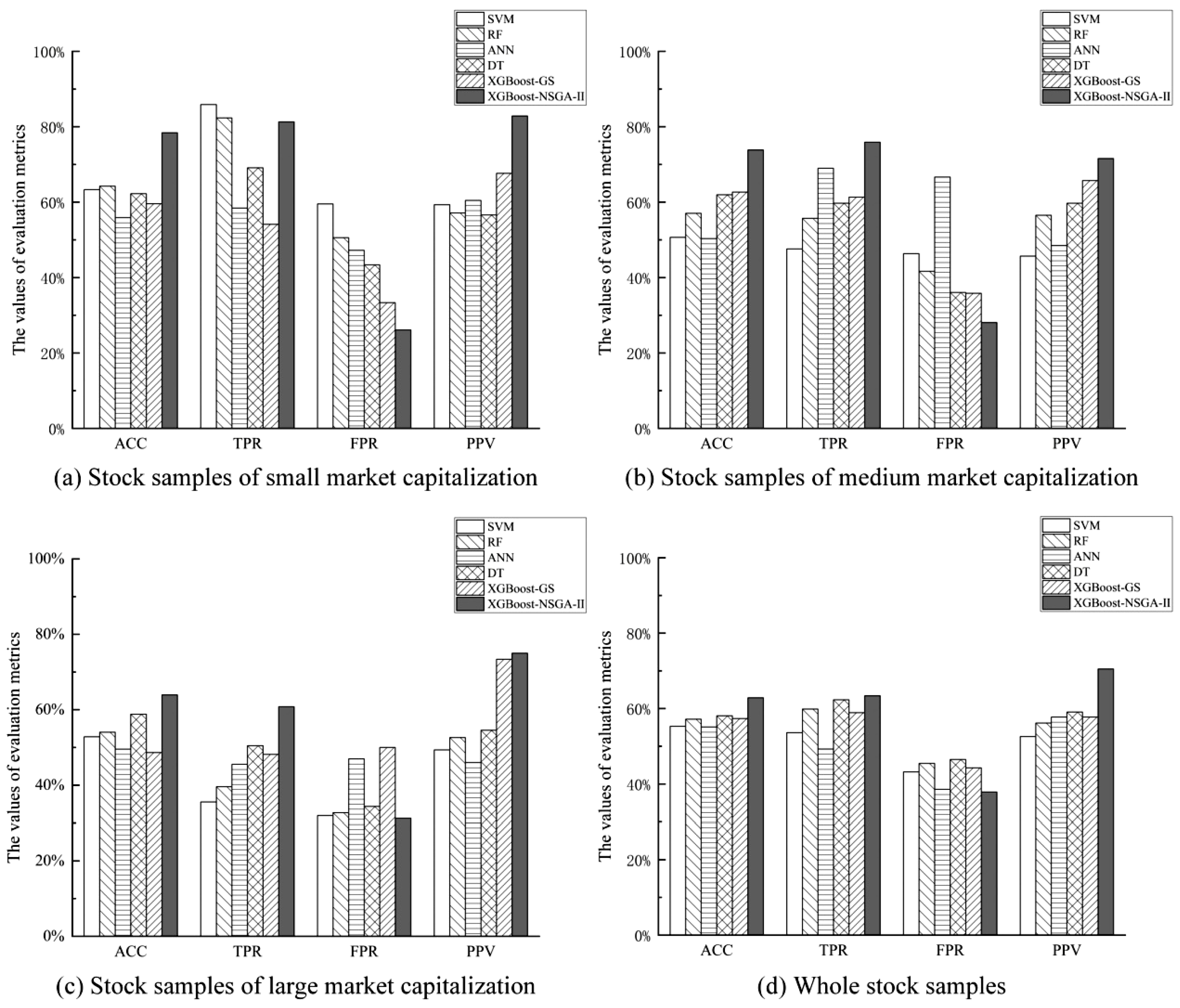
First, we focus on the prediction accuracy of stock price crashes by each forecasting method. Among all the evaluation indicators, accuracy (ACC) is the correctness of the model for predicting stock-price-crash samples and non-stock-crash samples, which can reflect the accuracy of the prediction methods comprehensively. From the ACC results, we could conclude the following findings: (1) The ACCs of the small-capitalization, medium-capitalization, large-capitalization, and whole datasets were 78.41%, 73.83%, 63.93%, and 62.88%, respectively. Therefore, from the results of four categories divided by market capitalization size, it is found that the proposed XGBoost–NSGA-II prediction model produced the greatest predictive accuracy among all the investigated methods. (2) Compared to the other benchmark methods, the XGBoost model produced a better ACC in predicting stock price crashes, indicating that XGBoost was more effective in identifying stock price crashes. (3) The NSGA-II used for hyperparameter optimization of the XGBoost stock price crash prediction model successfully improved the predictive accuracy. Regarding the benchmark XGBoost–GS method that applied grid search for hyperparameter optimization of the XGBoost model: looking at all four datasets, i.e., small-capitalization, medium-capitalization, and large-capitalization, as well as the whole dataset, the method only obtained ACC results of 59.60%, 62.67%, 48.63%, and 57.34% respectively. Using the NSGA-II for hyperparameter optimization of the XGBoost model, the ACC results for the four datasets reached 78.41%, 73.83%, 63.93%, and 62.88%, all of which outperformed the prediction accuracy of the GS method. (4) The accuracy of the proposed model consistently generated the best ACC result for each category of different market capitalization, and it produced the largest ACC result for the small-capitalization company stocks.
Second, the prediction accuracy of the proposed method and benchmark methods are analyzed in terms of another evaluation measure: positive predictive value (PPV), which is the proportion of correct identifications of stock-price-crash samples. Similar to the ACC results, it is evident that the proposed XGBoost–NSGA-II method generated a higher PPV than all the benchmark methods. For the proposed method, its PPV results for the small, medium, and large market capitalization datasets were 82.86%, 71.59%, and 75.00%, respectively. For the whole dataset, the proposed method obtained a PPV value of 70.51%. Therefore, it could be concluded that the proposed method performed best in predicting stock price crashes for the small-capitalization samples.
Additionally, for security market regulators to warn of stock price crashes effectively, an excellent warning model should produce not only a high predictive accuracy for stock crash prediction but also an excellent identification efficiency. Among the evaluation measures, TPR and FPR are commonly used to measure prediction efficiency. The TPR reflects the proportion of crash samples that are correctly predicted. Thus, a larger TPR result indicates the model is more efficient in predicting stock price crashes. In addition, FPR represents the proportion of non-crash samples that are incorrectly predicted as stock-crash samples in all non-crash samples; a smaller FPR value indicates a lower error rate, which could represent more efficiency in predicting stock price crashes. Therefore, TPR and FPR are used as efficiency evaluation indicators for the prediction models to compare the prediction efficiency of different methods. From the performances shown in Table 6, we could obtain the following findings: (1) The TPR of the proposed XGBoost–NSGA-II method was 81.31% in the small-capitalization samples. Although it was not the largest among all the methods, it was only 4.57% lower than the TPR of the SVM-based method. However, it is not sufficient to use TPR alone to reflect the predictive efficiency of a forecasting model. In the small-capitalization samples, the FPR of the proposed method was only 26.09%, which was the lowest value. Therefore, based on the results of TPR and FPR for prediction efficiency evaluation, the XGBoost–NSGA-II prediction model had both a high TPR and a low FPR in the small-capitalization samples, which indicates that it had an extraordinary predictive ability in terms of prediction efficiency. (2) The XGBoost–NSGA-II prediction model produced the largest TPR values in the medium-capitalization sample and the large-capitalization sample, which were 75.90% and 60.81%, respectively. Additionally, the proposed method also had the lowest FPR of 28.09% in the medium-capitalization sample. For the large market capitalization sample, the FPR was only 31.25%, which was also the lowest one. Therefore, in terms of these two evaluation indicators of stock price crash prediction efficiency, the proposed XGBoost–NSGA-II method performed best in terms of predictive efficiency in both the medium and large market capitalization samples. (3) In the whole dataset, the XGBoost–NSGA-II prediction model obtained the greatest prediction efficiency, with a TPR of 63.40% and an FPR of 37.86%. In summary, compared with the benchmark methods, the proposed XGBoost–NSGA-II method could predict stock price crashes with the highest predictive efficiency.
According to the results comparison of the prediction accuracy and efficiency of the prediction models, it could be concluded that the proposed XGBoost–NSGA-II method performed best compared to other machine learning-based algorithms. Next, we further analyze the prediction results of the proposed method on different market capitalization datasets based on these four evaluation indicators (see Table 7 and Figure 5). First, it is evident from the experimental results that the XGBoost–NSGA-II stock price crash prediction model had the worst prediction results in the overall dataset based on the analysis of the four evaluation metrics. Therefore, it could be concluded from the results that for the proposed model, dividing the dataset by market capitalization size and then training the model could improve the prediction accuracy and efficiency. Next, we focus on the prediction accuracy of the proposed method: the proposed XGBoost–NSGA-II model generates the greatest ACC (78.41%) on the samples of the small-capitalization dataset. Additionally, positive predictive value (PPV) shows the proportion of actual crash samples that are correctly predicted by the method. Therefore, in practice, it is often used as an evaluation measure for prediction methods, and a larger PPV value generally indicates that a model is more accurate in predicting the occurrence of a stock price crash. The PPV of the XGBoost–NSGA-II model was up to 82.86% in the small-capitalization dataset, which was 11.27% larger than the PPV of the medium-capitalization dataset, and it was 7.86% larger than the PPV of the large-capitalization dataset. Therefore, we could conclude that the proposed XGBoost–NSGA-II method performed best in the small-capitalization sample dataset.
We then focus on the prediction efficiency of the proposed prediction model. In the small-capitalization dataset, the TPR of the XGBoost–NSGA-II method reached 81.31%, which was 5.41% larger than that in the medium-capitalization dataset and 20.5% larger than that in the large-capitalization dataset. Moreover, XGBoost–NSGA-II produced the lowest FPR value (26.09%) for the small-capitalization dataset. Therefore, similar to the prediction accuracy results, it is obvious that the proposed XGBoost–NSGA-II method also produced greater prediction efficiency in the small-capitalization dataset than in other datasets.
In conclusion, it was found that compared to other machine learning-based methods, the XGBoost–NSGA-II stock crash prediction model successfully generated the best performances in terms of prediction accuracy and efficiency for predicting stock price crashes. Additionally, for samples from different market capitalization groups, the proposed model performed best in the small-capitalization dataset. This conclusion is consistent with the findings in the previous literature [73]. One possible reason for this could be that the stock price volatility of companies with small capitalizations is more sensitive to changes in their financial indicators compared to companies with medium and large market capitalizations [74].
5.3. Feature Importance Analysis
Figure 6 shows the features that ranked in the top 10 for importance for the experiments on each dataset. The features are selected by the Gain values of each feature in the training step of the XGBoost model. In each sub-figure of Figure 6, the horizontal axis shows the Gain value of each feature, and the vertical axis shows the name of each feature. In Figure 6a, for the experiment on the whole dataset, it is clear that the total assets growth rate (c1) contributed more than other features to the predictions by the proposed XGBoost–NSGA-II method. Additionally, after dividing the whole dataset according to market capitalization size and then performing the experiments individually, it could be found that financial indicators show apparent differences in their contributions to stock price crash predictions by the proposed XGBoost–NSGA-II method for samples of different market capitalization sizes. For instance, in the experiment on the large-capitalization dataset, the long-term debt to asset ratio (a6) and the working capital over total assets ratio (e3) were the features that contributed most to the prediction results of the proposed method, while the fixed assets turnover ratio (b5) was the feature that contributed most to the prediction results in the medium-capitalization dataset. However, before the whole dataset was divided and investigated separately, the contribution of those features to the prediction results of the proposed model was not critical in the experiment on the whole dataset. The largest Gain value in the experiment of the small-capitalization dataset remained that of the total assets growth rate (c1). Therefore, through the investigation of feature importance for the prediction method, it is possible for market regulators to select the critical financial indicators for stock samples in different market capitalization groups, which are beneficial for them in predicting stock price crashes in a more targeted and efficient way. For the small-capitalization samples, the key financial indicator for predicting the occurrence of a stock crash was the total assets growth rate (c1), a measure indicator showing the growing ability of a company. The key financial indicator for predicting a stock crash in the medium-capitalization dataset was the fixed assets turnover ratio (b5), which is the operating capacity of a company. For the large-capitalization samples, the key financial indicators for predicting the occurrence of a stock price crash included the long-term debt to asset ratio (a6), which measures a company’s debt-paying ability, as well as the working capital over total assets ratio (e3) that reflects its capital structure.
5.4. Results of the SHAP Approach
In Section 5.3, the importance of the most critical features is ranked and analyzed by the Gain values generated during the model training of XGBoost. Although the Gain value measures the magnitude of the influence of the features on the stock price crash predictions of the model, it is still challenging to understand the influence direction of each feature on the prediction results. Therefore, the SHAP method is further adopted to specifically analyze the contributions of the critical features of each dataset to the respective model predictions [49,75]. Considering that the proposed XGBoost–NSGA-II method generated the best prediction results in the category of small-capitalization samples, we focus on and analyze the critical features in the small-capitalization dataset by using the SHAP method. Figure 7 shows the top 10 critical features for prediction in the small-capitalization dataset, ranked by the importance of each feature. The vertical axis represents the feature name in the dataset, and each point in the graph is one variable of the feature. The colors of the points indicate the deviation of the feature value for each stock variable, and the horizontal axis represents the SHAP values of the predicted samples of each feature.
From Figure 7, we can observe the relationships between SHAP values and feature values for the critical variables. For c1 (total assets growth rate) and e2 (cash to assets ratio), the larger those feature values, the larger the SHAP values, which means a higher possibility of a stock price crash. Additionally, the larger the feature values of d4 (gross profit margin ratio), e1 (current assets to total assets ratio), and e4 (fixed assets ratio), the lower the stock price crash possibility. We then focus on the top four important features, and SHAP dependence plots are drawn for the features for further analysis of the influences of the feature values on the prediction results.
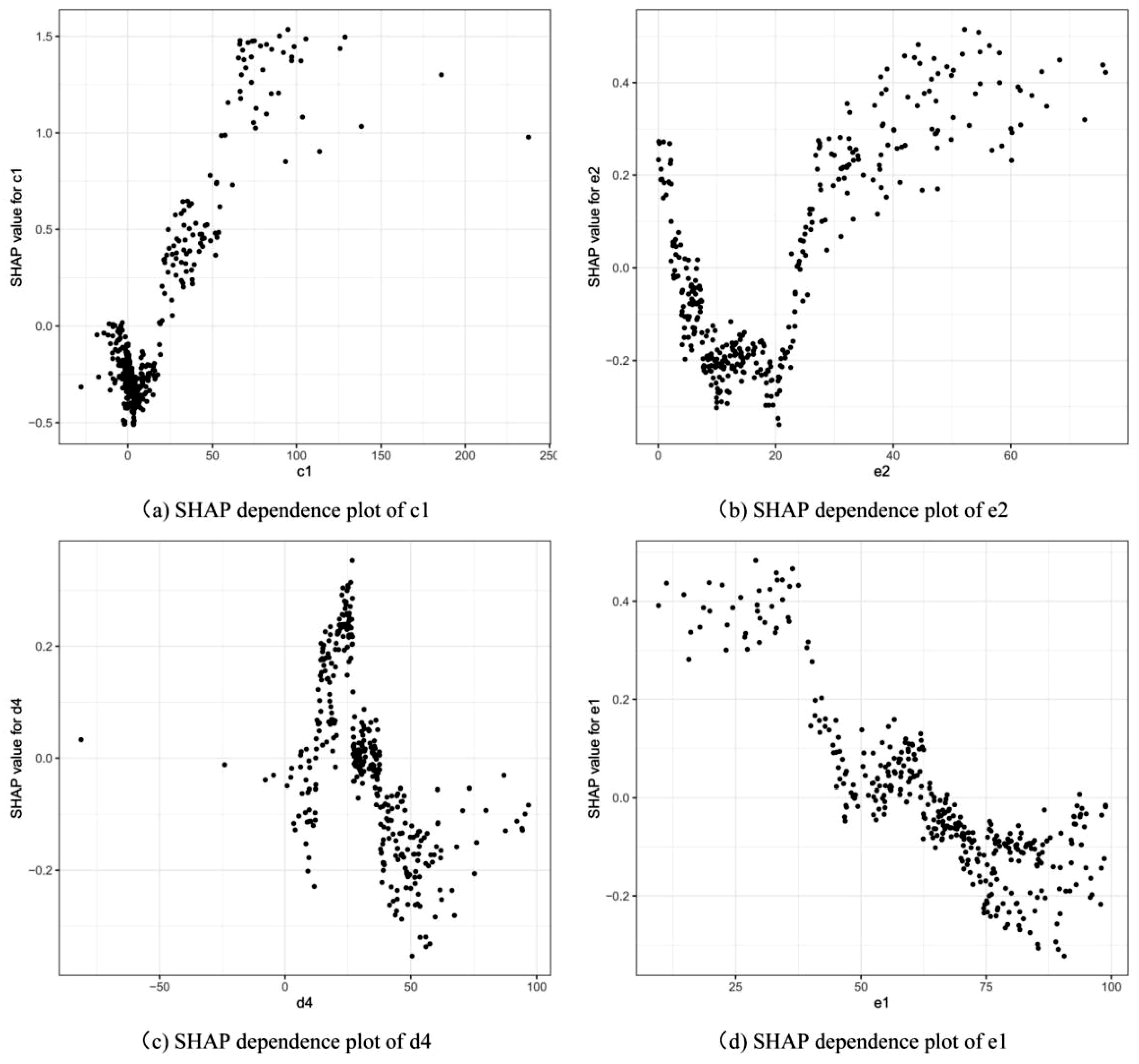
Figure 8 represents the SHAP dependence plots of the top four critical features (c1, e2, d4, and e1) for stock price crash prediction in the small-capitalization samples. They reflect the SHAP values of all corresponding samples for those features, from which it is possible to analyze how the SHAP value of each feature changes as the feature value changes. The vertical axis of each subplot in Figure 8 represents the SHAP values for the stock samples, and the horizontal axis represents the feature value. First, when the feature value of c1 (total assets growth rate) gradually became larger from the negative values, its SHAP value was gradually decreased, indicating that as the feature value of c1 gradually rose, the possibility of a stock price crash gradually decreased until the feature value increased to near zero. As the feature value continued to increase, the SHAP value gradually increased, indicating that when the value of c1 was greater than zero, the larger the feature value of c1, the higher possibility of a stock price crash. The possibility of a stock price crash decreased as e2 (cash to assets ratio) grew from 0% to approximately 18%, while the possibility of stock price crash became greater as the feature value of e2 increased from about 18% to 80%. For d4 (gross profit margin ratio), the possibility of a stock price crash gradually increased as its feature value gradually increased from a negative value to approximately 25%, while the stock price crash possibility gradually decreased as the feature value of d4 continued to increase from about 25% to approximately 100%. Furthermore, as e1 (current assets to total assets ratio) gradually increased from 0% to about 100%, the stock price crash possibility continuously decreased. By analyzing the relationship between the feature values of the above four critical features and their SHAP values, we could determine the specific influence of changes in feature values on the prediction results. The results could therefore be utilized to interpret the proposed prediction model, thus improving the interpretability of the proposed model.
5.5. Managerial Insight
The proposed XGBoost–NSGA-II–SHAP method could provide investors and market regulators with managerial insight. Firstly, the proposed method could be used as a reference for market investors to reduce trading risk. Secondly, market regulators could take appropriate actions (for instance, limiting the trading volume of a stock that has a large possibility of a stock price crash) in advance to control trading risk. Thirdly, the results of the Gain values and SHAP values could help market investors and regulators understand which financial variables are the main features for predicting the stock price crashes of individual stocks. In this regard, the proposed model could be used as an alternative method to provide market regulations with guidance on the crucial features within the financial indicators.
6. Conclusions
In this study, we have proposed a novel method named XGBoost–NSGA-II–SHAP for the prediction and explanation of stock price crashes in the Chinese security market. The proposed method employs financial indicators as features to predict stock price crashes. To explain the proposed prediction model, the critical financial indicators are analyzed for the different market capitalization samples, and the influences of those feature values on the model’s prediction results are also explained. According to the experimental results, the following main conclusions could be generated: (1) Compared to other classical machine learning-based methods, XGBoost produced the best prediction results for stock price crash prediction. (2) The NSGA-II was adopted for multi-objective optimization of the hyperparameters of the XGBoost method, which not only improved the accuracy of the model in identifying stock price crashes, but also successfully enhanced the efficiency of stock price crash warnings. (3) Compared to the benchmark methods, the proposed XGBoost–NSGA-II method generated the best prediction accuracy and efficiency. In addition, comparing the performance of the proposed models in different market capitalization datasets, it could also be found that the proposed XGBoost–NSGA-II method for stock price crash prediction obtained better prediction results in the small-capitalization dataset. (4) For the small-capitalization samples, the critical feature for stock price crashes prediction is the total assets growth rate, while for the stock samples with medium capitalization, the critical feature is the fixed assets turnover. Moreover, for the large-capitalization samples, the key indicators are the long-term debt to asset ratio and the working capital over total assets ratio. (5) For the top four critical financial indicators from the experiments on small-capitalization samples, the stock price crash possibility initially decreased and then increased as the values of the total assets growth rate and the cash to assets ratio increased. As the value of the gross profit margin ratio increased, the stock price crash possibility initially increased and then decreased. For the current assets to total assets ratio feature, the stock price crash possibility was continuously and gradually reduced as its value increased.
However, there are still several limitations of this study: (1) This study used only the financial indicators of the firms as the features for stock price crash prediction. (2) We studied only the stock price crashes of individual stocks of the Chinese stock market. (3) In the experiments, we divided the group of stocks only from the perspective of company capitalization.
There are several possible research directions for other researchers to expand on this research. (1) Other scholars could consider using other factors, such as investor sentiments, market trading indicators, war factors, COVID-19, and so on, as the prediction features for predicting stock price crash risks. (2) Other scholars can also apply the method proposed in this study to research on price crashes in other stock markets or financial markets, such as futures markets and foreign exchange markets, to predict and explain their price crashes. (3) Other researchers could divide the stocks from other perspectives, such as industries or markets (Main Board market or Second Board market).
Author Contributions
Conceptualization, S.D. (Shangkun Deng) and Z.L.; methodology, S.D. (Shangkun Deng) and Y.Z.; validation, Y.Z. and S.D. (Shangkun Deng); formal analysis, S.D. (Shangkun Deng) and Z.L.; investigation, Y.Z. and S.D. (Shuangyang Duan); resources, S.D. (Shangkun Deng); data curation, Y.Z. and Z.F.; writing—original draft preparation, Y.Z.; writing—review and editing, S.D. (Shangkun Deng), Z.F. and Z.L.; visualization, Y.Z. and S.D. (Shuangyang Duan); supervision, S.D. (Shangkun Deng). All authors have read and agreed to the published version of the manuscript.
Funding
This work is supported by Natural Science Foundation of Hubei Province (grant number 2021CFB175), Philosophy and Social Science Research Project of the Department of Education of Hubei Province (grant number 21Q035), and Natural Science Foundation of Yichang City (grant number A22-3-011).
Institutional Review Board Statement
Not applicable.
Informed Consent Statement
Not applicable.
Data Availability Statement
Publicly available datasets were analyzed in this study. This data can be found here: [http://www.csmar.com] and [http://www.resset.cn/databases].
Acknowledgments
The authors are grateful to the editors and anonymous reviewers for their comments and discussions.
Conflicts of Interest
The authors declare no conflict of interest.
References
- Jin, L.; Myers, S.C. R2 around the world: New theory and new tests. J. Financ. Econ. 2006, 79, 257–292. [Google Scholar] [CrossRef] [Green Version]
- Farmer, R.E.A. The stock market crash of 2008 caused the Great Recession: Theory and evidence. J. Econ. Dyn. Control 2012, 36, 693–707. [Google Scholar] [CrossRef]
- Zhou, L.; Huang, J. Investor trading behaviour and stock price crash risk. Int. J. Financ. Econ. 2019, 24, 227–240. [Google Scholar] [CrossRef] [Green Version]
- Bond, S.; Devereux, M. Financial volatility, the stock market crash and corporate investment. Fisc. Stud. 1988, 9, 72–80. [Google Scholar] [CrossRef]
- Bleck, A.; Liu, X. Market transparency and the accounting regime. J. Account. Res. 2007, 45, 229–256. [Google Scholar] [CrossRef]
- Hutton, A.P.; Marcus, A.J.; Tehranian, H. Opaque financial reports, R2, and crash risk. J. Financ. Econ. 2009, 94, 67–86. [Google Scholar] [CrossRef]
- Kim, J.B.; Li, Y.; Zhang, L. Corporate tax avoidance and stock price crash risk: Firm-level analysis. J. Financ. Econ. 2011, 100, 639–662. [Google Scholar] [CrossRef]
- Xu, N.; Li, X.; Yuan, Q.; Chan, K.C. Excess perks and stock price crash risk: Evidence from China. J. Corp. Financ. 2014, 25, 419–434. [Google Scholar] [CrossRef]
- Li, E.Z.J.; Yu, H.; Lin, H.; Chen, G. Correlation analysis between stock prices and four financial indexes for some listed companies of mainland China. In Proceedings of the 2017 10th International Congress on Image and Signal Processing, BioMedical Engineering and Informatics (CISP-BMEI 2017), Shanghai, China, 14–16 October 2017; 2018; pp. 1–5. [Google Scholar] [CrossRef]
- Kaizoji, T.; Miyano, M. Stock market crash of 2008: An empirical study of the deviation of share prices from company fundamentals. Appl. Econ. Lett. 2019, 26, 362–369. [Google Scholar] [CrossRef] [Green Version]
- Wang, B.; Ho, K.C.; Liu, X.; Gu, Y. Industry cash flow volatility and stock price crash risk. Manag. Decis. Econ. 2022, 43, 356–371. [Google Scholar] [CrossRef]
- Feltham, G.A.; Ohlson, J.A. Valuation and clean surplus accounting for operating and financial activities. Contemp. Account. Res. 1995, 11, 689–731. [Google Scholar] [CrossRef]
- Jiang, J.; Chang, R. Relationship between key financial statements and stock price of GEM listed companies. Sci. Tec. Ind. 2013, 13, 69–73. [Google Scholar] [CrossRef]
- Xu, M.; Liu, X. The correlation between financial indexes and stock prices in ChiNext—Based on manufacturing and IT industry. Stat. Appl. 2018, 7, 281–290. [Google Scholar] [CrossRef]
- Sornette, D. Critical market crashes. Phys. Rep. 2003, 378, 1–98. [Google Scholar] [CrossRef] [Green Version]
- Herrera, R.; Schipp, B. Self-exciting extreme value models for stock market crashes. In Statistical Inference, Econometric Analysis and Matrix Algebra; Schipp, B., Kräer, W., Eds.; Physica-Verlag HD: Heidelberg, Germany, 2009; pp. 209–231. [Google Scholar] [CrossRef]
- Lleo, S.; Ziemba, W.T. Stock market crashes in 2007-2009: Were we able to predict them? Quant. Financ. 2012, 12, 1161–1187. [Google Scholar] [CrossRef]
- Dai, B.; Zhang, F.; Tarzia, D.; Ahn, K. Forecasting financial crashes: Revisit to log-periodic power law. Complexity 2018, 2018, 4237471. [Google Scholar] [CrossRef]
- Kurz-Kim, J.R. Early warning indicator for financial crashes using the log periodic power law. Appl. Econ. Lett. 2012, 19, 1456–1469. [Google Scholar] [CrossRef]
- Pele, D.T.; Mazurencu-Marinescu, M. An econophysics approach for modeling the behavior of stock market bubbles: Case study for the bucharest stock exchange. In Emerging Macroeconomics: Case Studies–Central and Eastern Europe; Nova Science Publishers: London, UK, 2013; pp. 81–90. [Google Scholar]
- Zhang, Y.J.; Yao, T. Interpreting the movement of oil prices: Driven by fundamentals or bubbles? Econ. Model. 2016, 55, 226–240. [Google Scholar] [CrossRef]
- Tsuji, C. Is volatility the best predictor of market crashes? Asia-Pac. Financ. Mark. 2003, 10, 163–185. [Google Scholar] [CrossRef]
- Jones, J.S.; Kincaid, B. Can the correlation among Dow 30 stocks predict market declines? Evidence from 1950 to 2008. Manag. Financ. 2014, 40, 33–50. [Google Scholar] [CrossRef]
- Reza Razavi Araghi, S.M.; Lashgari, Z. The effect of internal control material weaknesses on future stock price crash risk: Evidence from Tehran Stock Exchange (TSE). Int. J. Account. Res. 2017, 5, 1–5. [Google Scholar] [CrossRef]
- Ouyang, H.B.; Huang, K.; Yan, H. Prediction of financial time series based on LSTM Neural Network. Chinese J. Manag. Sci. 2020, 28, 27–35. [Google Scholar] [CrossRef]
- Inthachot, M.; Boonjing, V.; Intakosum, S. Predicting SET50 index trend using artificial neural network and support vector machine. In Lecture Notes in Computer Science (including Subseries Lecture Notes in Artificial Intelligence and Lecture Notes in Bioinformatics); Springer: Durham, UK, 2015; pp. 404–414. [Google Scholar] [CrossRef]
- Jaiwang, G.; Jeatrakul, P. A forecast model for stock trading using support vector machine. In Proceedings of the 20th International Computer Science and Engineering Conference: Smart Ubiquitos Computing and Knowledge, ICSEC 2016, Chiang Mai, Thailand, 14–17 December 2016. [Google Scholar] [CrossRef]
- Chatzis, S.P.; Siakoulis, V.A.; Petropoulos, E.; Stavroulakis, N. Vlachogiannakis, Forecasting stock market crisis events using deep and statistical machine learning techniques. Expert Syst. Appl. 2018, 112, 353–371. [Google Scholar] [CrossRef]
- Ning, T.; Miao, D.; Dong, Q.; Lu, X. Wide and deep learning for default risk prediction. Comput. Sci. 2021, 48, 197–201. [Google Scholar] [CrossRef]
- Chen, T.; Guestrin, C. XGBoost: A scalable tree boosting system. In Proceedings of the 22nd ACM SIGKDD International Conference on Knowledge Discovery and Data Mining, San Francisco, CA, USA, 13–17 August 2016; pp. 785–794. [Google Scholar] [CrossRef] [Green Version]
- Guang, P.; Huang, W.; Guo, L.; Yang, X.; Huang, F.; Yang, M.; Wen, W.; Li, L. Blood-based FTIR-ATR spectroscopy coupled with extreme gradient boosting for the diagnosis of type 2 diabetes: A STARD compliant diagnosis research. Medicine 2020, 99, e19657. [Google Scholar] [CrossRef]
- Xie, Y.; Zhang, C.; Hu, X.; Zhang, C.; Kelley, S.P.; Atwood, J.L.; Lin, J. Machine learning sssisted synthesis of metal-organic nanocapsules. J. Am. Chem. Soc. 2020, 142, 1475–1481. [Google Scholar] [CrossRef] [Green Version]
- Huang, Q.; Xie, H. Research on the application of machine learning in stock index futures forecast—comparison and analysis based on BP neural network, SVM and XGBoost. Math. Pract. Th. 2018, 48, 297–307. [Google Scholar]
- Deng, S.; Huang, X.; Qin, Z.; Fu, Z.; Yang, T. A novel hybrid method for direction forecasting and trading of apple futures. Appl. Soft Comput. 2021, 110, 107734. [Google Scholar] [CrossRef]
- Deng, S.; Wang, X.H.J.; Qin, Z.; Fu, Z.; Wang, A.; Yang, T. A decision support system for trading in apple futures market using predictions fusion. IEEE Access 2021, 9, 1271–1285. [Google Scholar] [CrossRef]
- Gu, Y.; Zhang, D.; Bao, Z. A new data-driven predictor, PSO-XGBoost, used for permeability of tight sandstone reservoirs: A case study of member of chang 4+5, western Jiyuan Oilfield, Ordos Basin. J. Pet. Sci. Eng. 2021, 199, 108350. [Google Scholar] [CrossRef]
- Piehowski, P.D.; Sandoval, V.A.P.J.D.; Burnum, K.E.; Kiebel, G.R.; Monroe, M.E.; Anderson, G.A.; Camp, D.G.; Smith, R.D. STEPS: A grid search methodology for optimized peptide identification filtering of MS/MS database search results. Proteomics 2013, 13, 766–770. [Google Scholar] [CrossRef] [PubMed] [Green Version]
- Mandal, P.; Dey, D.; Roy, B. Indoor lighting optimization: A comparative study between grid search optimization and particle swarm optimization. J. Opt. 2019, 48, 429–441. [Google Scholar] [CrossRef]
- Adnan, M.N.; Islam, M.Z. Optimizing the number of trees in a decision forest to discover a subforest with high ensemble accuracy using a genetic algorithm. Knowl.-Based Syst. 2016, 110, 86–97. [Google Scholar] [CrossRef]
- Islam, M.Z.; Estivill-Castro, V.; Rahman, M.A.; Bossomaier, T. Combining K-MEANS and a genetic algorithm through a novel arrangement of genetic operators for high quality clustering. Expert Syst. Appl. 2018, 91, 402–417. [Google Scholar] [CrossRef]
- Raman, M.R.G.; Somu, N.; Kirthivasan, K.; Liscano, R.; Shankar Sriram, V.S. An efficient intrusion detection system based on hypergraph-Genetic algorithm for parameter optimization and feature selection in support vector machine. Knowl.-Based Syst. 2017, 134, 1–12. [Google Scholar] [CrossRef]
- Wang, Y.; Guo, Y. Application of improved XGBoost model in stock forecasting. Comput. Engine. Appl. 2019, 55, 202–207. [Google Scholar] [CrossRef]
- Ma, Y.; Yun, W. Research progress of genetic algorithm. Appl. Res. Comput. 2012, 29, 1201–1206. [Google Scholar] [CrossRef]
- Zhang, Y.; Liu, M. Adaptive directed evolved NSGA2 based node placement optimization for wireless sensor networks. Wirel. Networks 2020, 26, 3539–3552. [Google Scholar] [CrossRef]
- Parizad, A.; Hatziadoniu, K. Security/stability-based Pareto optimal solution for distribution networks planning implementing NSGAII/FDMT. Energy 2020, 192, 116644. [Google Scholar] [CrossRef]
- Ji, B.; Yuan, X.; Yuan, Y. Modified NSGA-II for solving continuous berth allocation problem: Using multiobjective constraint-handling strategy. IEEE Trans. Cybern. 2017, 47, 2885–2895. [Google Scholar] [CrossRef]
- González-Álvarez, D.L.; Vega-Rodríguez, M.A. Analysing the scalability of multiobjective evolutionary algorithms when solving the motif discovery problem. J. Glob. Optim. 2013, 57, 467–497. [Google Scholar] [CrossRef]
- Cao, R.; Liao, B.; Li, M.; Sun, R. Predicting prices and analyzing features of online short-term rentals based on XGBoost. Data Anal. Knowl. Disc. 2021, 5, 51–65. [Google Scholar] [CrossRef]
- Lundberg, S.M.; Lee, S.I. Consistent feature attribution for tree ensembles. In Proceedings of the 2017 ICML Workshop on Human Interpretability in Machine Learning, Sydney, Australia, 10 August 2017; pp. 31–38. [Google Scholar]
- Lundberg, S.M.; Lee, S.I. A unified approach to interpreting model predictions. Adv. Neural Inf. Processing Syst. 2017, 30, 4766–4775. [Google Scholar]
- Heuillet, A.; Couthouis, F.; Díaz-Rodríguez, N. Explainability in deep reinforcement learning. Knowl.-Based Syst. 2021, 214, 106685. [Google Scholar] [CrossRef]
- Li, J.; Shi, H.; Hwang, K.S. An explainable ensemble feedforward method with Gaussian convolutional filter. Knowl.-Based Syst. 2021, 225, 107103. [Google Scholar] [CrossRef]
- Parsa, A.B.; Movahedi, A.; Taghipour, H.; Derrible, S.; Mohammadian, A.K. Toward safer highways, application of XGBoost and SHAP for real-time accident detection and feature analysis. Accid. Anal. Prev. 2020, 136, 105405. [Google Scholar] [CrossRef] [PubMed]
- Jin, X.; Chen, Z.; Yang, X. Economic policy uncertainty and stock price crash risk. Account. Financ. 2019, 58, 1291–1318. [Google Scholar] [CrossRef]
- Yu, J.; Mai, D. Political turnover and stock crash risk: Evidence from China. Pac. Basin Financ. J. 2020, 61, 101324. [Google Scholar] [CrossRef]
- Schneider, G.; Troeger, V.E. War and the world economy: Stock market reactions to international conflicts. J. Confl. Resolut. 2006, 50, 623–645. [Google Scholar] [CrossRef]
- Baek, S.; Mohanty, S.K.; Glambosky, M. COVID-19 and stock market volatility: An industry level analysis. Financ. Res. Lett. 2020, 37, 101748. [Google Scholar] [CrossRef]
- Pourmansouri, R.; Mehdiabadi, A.; Shahabi, V.; Spulbar, C.; Birau, R. An investigation of the link between major shareholders’ behavior and corporate governance performance before and after the COVID-19 pandemic: A case study of the companies listed on the Iranian stock market. J. Risk Financ. Manag. 2022, 15, 208. [Google Scholar] [CrossRef]
- Aslam, F.; Mohmand, Y.T.; Ferreira, P.; Memon, B.A.; Khan, M.; Khan, M. Network analysis of global stock markets at the beginning of the coronavirus disease (COVID-19) outbreak. Borsa Istanb. Rev. 2020, 20, S49–S61. [Google Scholar] [CrossRef]
- Goldberg, D.E. Genetic Algorithms in Search, Optimization, and Machine Learning; Addison Wesley: Boston, MA, USA, 1989. [Google Scholar] [CrossRef]
- Srinivas, N.; Deb, K. Muiltiobjective optimization using nondominated sorting in genetic algorithms. Evol. Comput. 1994, 2, 221–248. [Google Scholar] [CrossRef]
- Deb, K.; Pratap, A.; Agarwal, S.; Meyarivan, T. A fast and elitist multiobjective genetic algorithm: NSGA-II. IEEE Trans. Evol. Comput. 2002, 6, 182–197. [Google Scholar] [CrossRef] [Green Version]
- Shapley, L.S. 17. A Value for n-Person Games. In Contributions to the Theory of Games (AM-28); Princeton University Press: Princeton, NJ, USA, 2016; Volume II, pp. 307–318. [Google Scholar] [CrossRef]
- Bogetoft, P.; Hougaard, J.L.; Smilgins, A. Applied cost allocation: The DEA-Aumann-Shapley approach. Eur. J. Oper. Res. 2016, 254, 667–678. [Google Scholar] [CrossRef] [Green Version]
- Duan, X.; Zhan, J. Opposite Effects of intra-group and inter-group rivalries: A study based on the partitioning effects of mobility barriers. Chin. J. Manag. Sci. 2015, 23, 125–133. [Google Scholar] [CrossRef]
- Chen, J.; Hong, H.; Stein, J.C. Forecasting crashes: Trading volume, past returns, and conditional skewness in stock prices. J. Financ. Econ. 2001, 61, 345–381. [Google Scholar] [CrossRef] [Green Version]
- Kim, J.B.; Li, Y.; Zhang, L. CFOs versus CEOs: Equity incentives and crashes. J. Financ. Econ. 2011, 101, 713–730. [Google Scholar] [CrossRef]
- Wang, K.; Feng, X.; Liu, C. Wave filed separation of fast-slow shear waves by Pearson correlation coefficient method. Glob. Geol. 2012, 31, 371–376. [Google Scholar] [CrossRef]
- Xu, J.; Tang, B.; He, H.; Man, H. Semisupervised feature selection based on relevance and redundancy criteria. IEEE Trans. Neural Networks Learn. Syst. 2017, 28, 1974–7984. [Google Scholar] [CrossRef] [PubMed]
- Budholiya, K.; Shrivastava, S.K.; Sharma, V. An optimized XGBoost based diagnostic system for effective prediction of heart disease. J. King Saud Univ.-Comput. Inf. Sci. 2020, 34, 4514–4523. [Google Scholar] [CrossRef]
- Ryu, S.E.; Shin, D.H.; Chung, K. Prediction model of dementia risk based on XGBoost using derived variable extraction and hyper parameter optimization. IEEE Access 2020, 8, 177708–177720. [Google Scholar] [CrossRef]
- Deng, S.; Wang, C.; Fu, Z.; Wang, M. An intelligent system for insider trading identification in Chinese security market. Comput. Econ. 2021, 57, 593–616. [Google Scholar] [CrossRef]
- Salisu, A.A.; Swaray, R.; Oloko, T.F. US stocks in the presence of oil price risk: Large cap vs. small cap. Econ. Bus. Lett. 2017, 6, 116–124. [Google Scholar] [CrossRef] [Green Version]
- Chen, Z.; Ru, J. Herding and capitalization size in the Chinese stock market: A micro-foundation evidence. Empir. Econ. 2021, 60, 1895–1911. [Google Scholar] [CrossRef]
- Rodríguez-Pérez, R.; Bajorath, J. Interpretation of compound activity predictions from complex machine learning models using local approximations and shapley values. J. Med. Chem. 2020, 63, 8761–8777. [Google Scholar] [CrossRef] [PubMed]
Figure 1.
The main procedures of the NSGA-II.
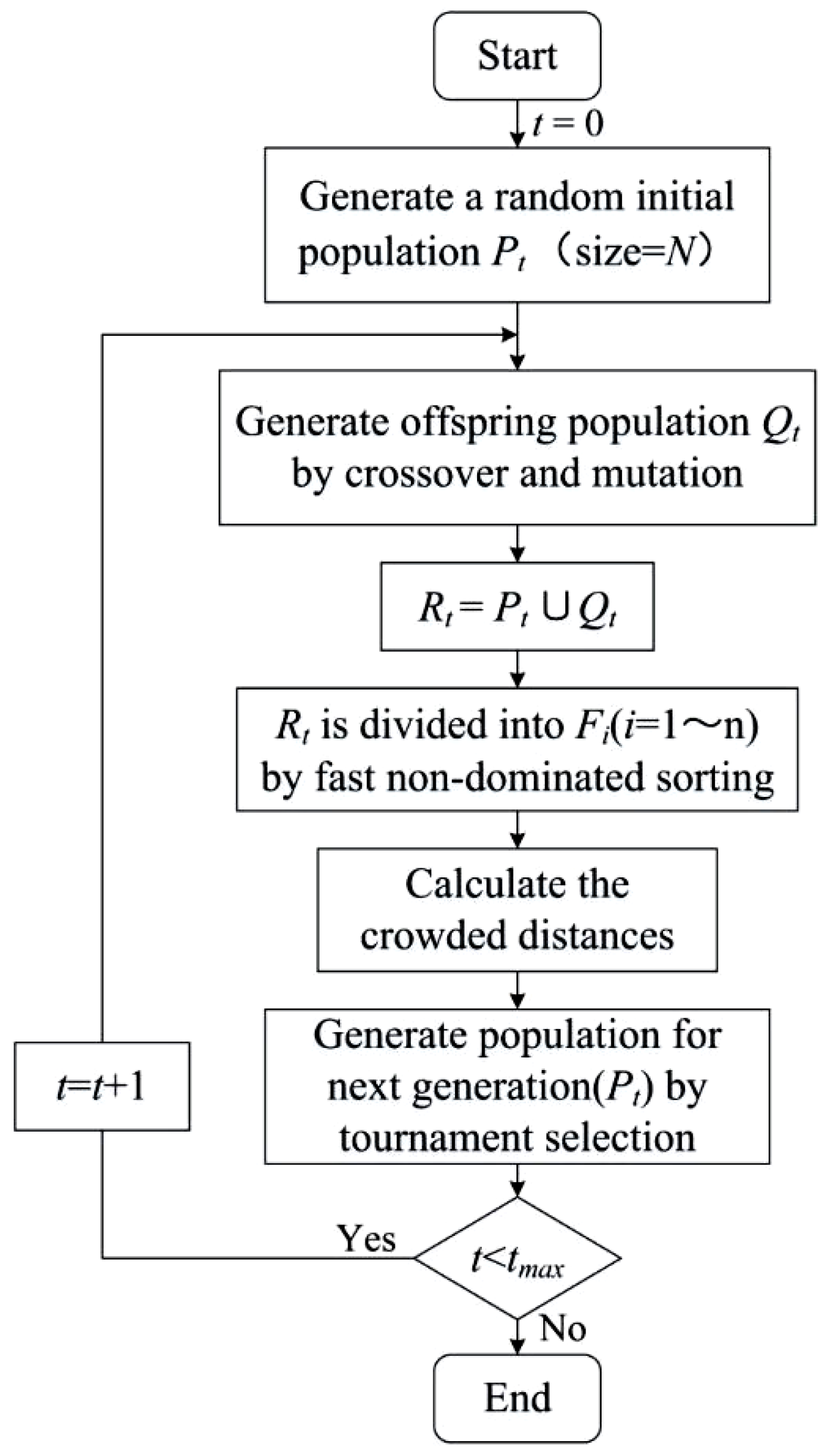
Figure 2.
The main components and procedures of the proposed method for predicting stock price crashes.
Figure 2.
The main components and procedures of the proposed method for predicting stock price crashes.
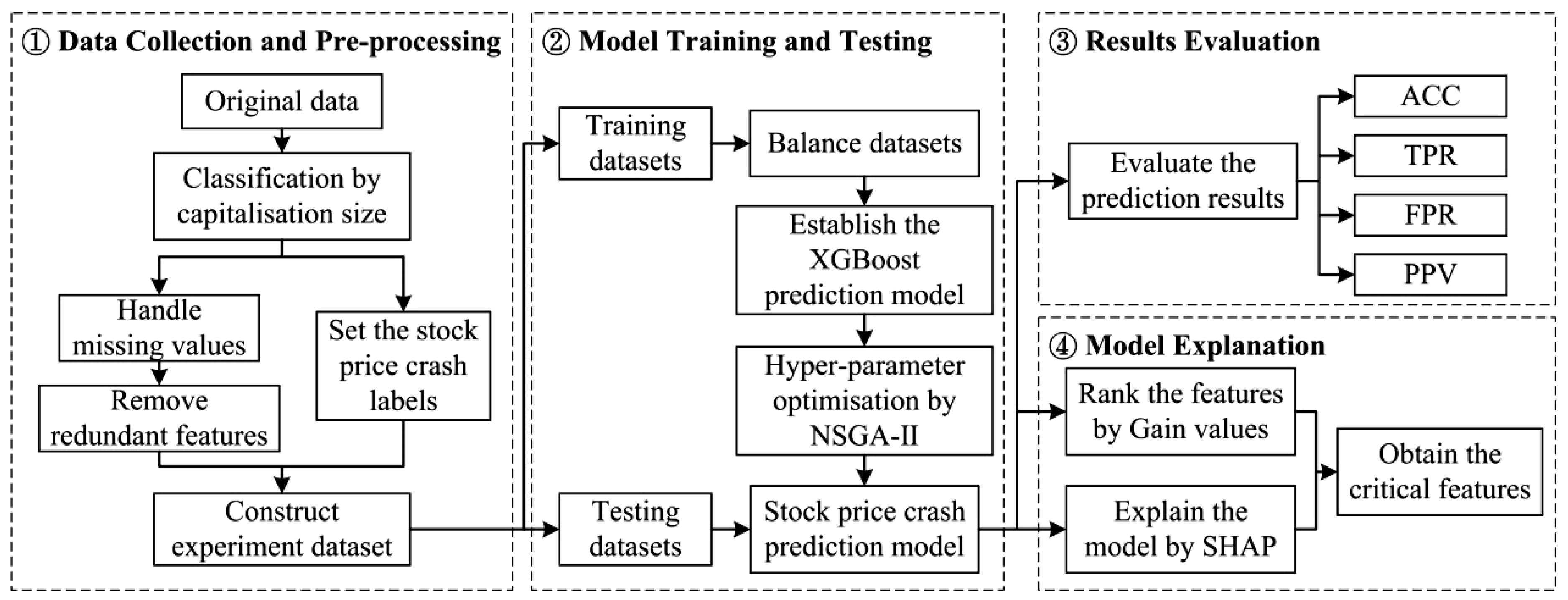
Figure 3.
Correlation tests results of financial indicator features in different categories of market capitalization.
Figure 3.
Correlation tests results of financial indicator features in different categories of market capitalization.
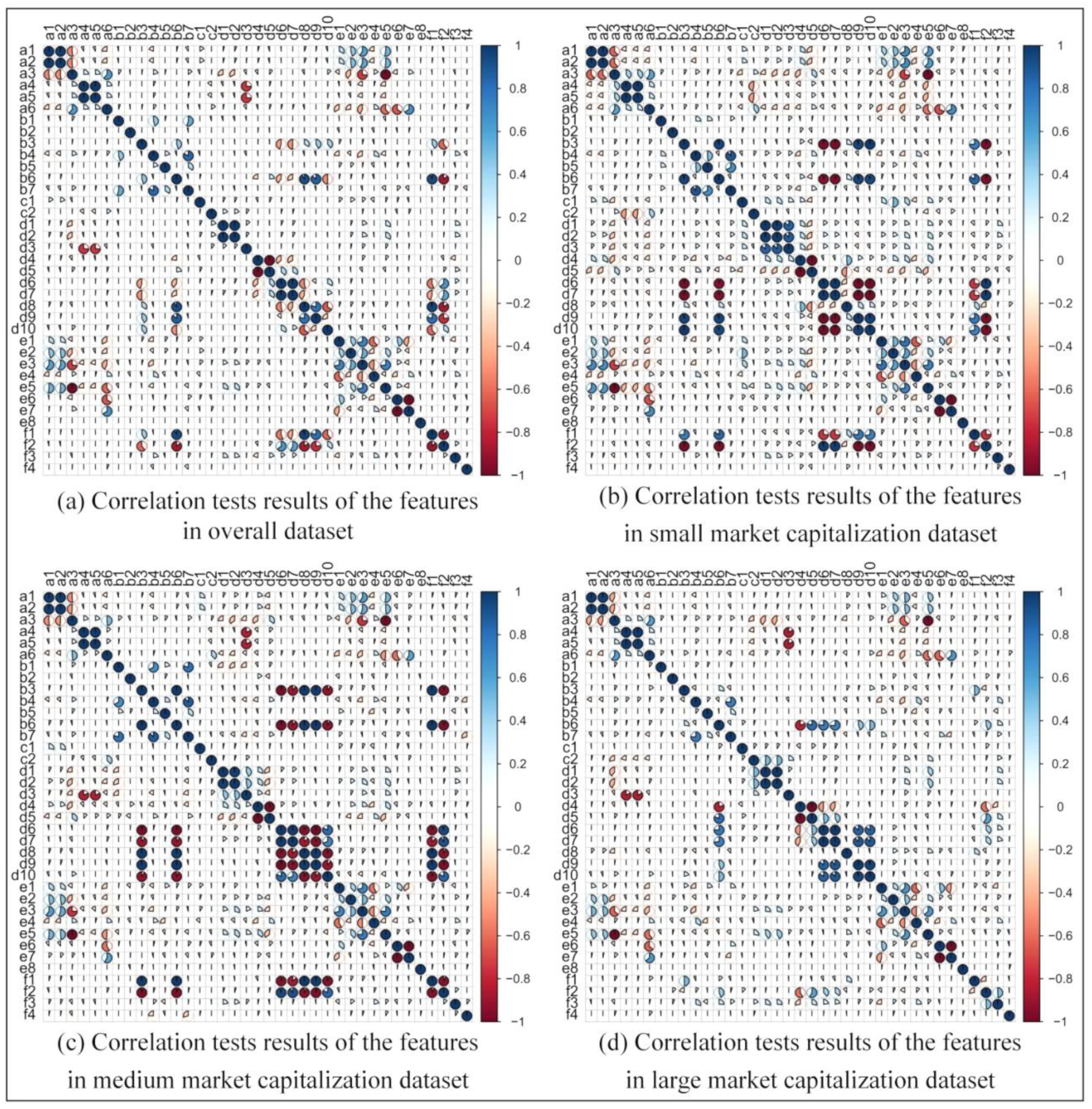
Figure 4.
Results of stock price crash prediction for the proposed method and benchmarks.

Figure 5.
Results of the proposed method for stock price crash prediction on four datasets with different market capitalization sizes.
Figure 5.
Results of the proposed method for stock price crash prediction on four datasets with different market capitalization sizes.
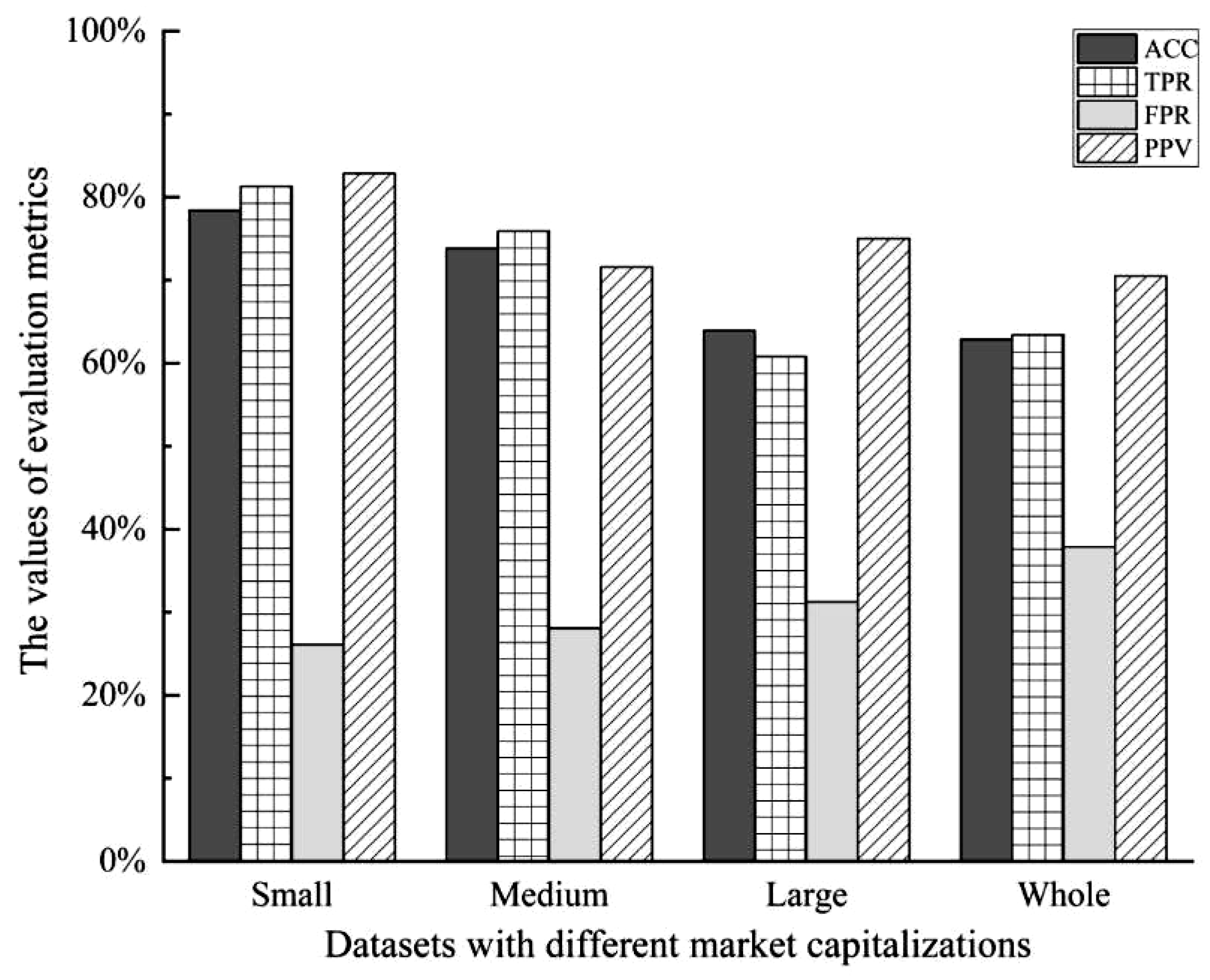
Figure 6.
The top 10 most important features for the proposed XGBoost–NSGA-II method for different market capitalization datasets.
Figure 6.
The top 10 most important features for the proposed XGBoost–NSGA-II method for different market capitalization datasets.
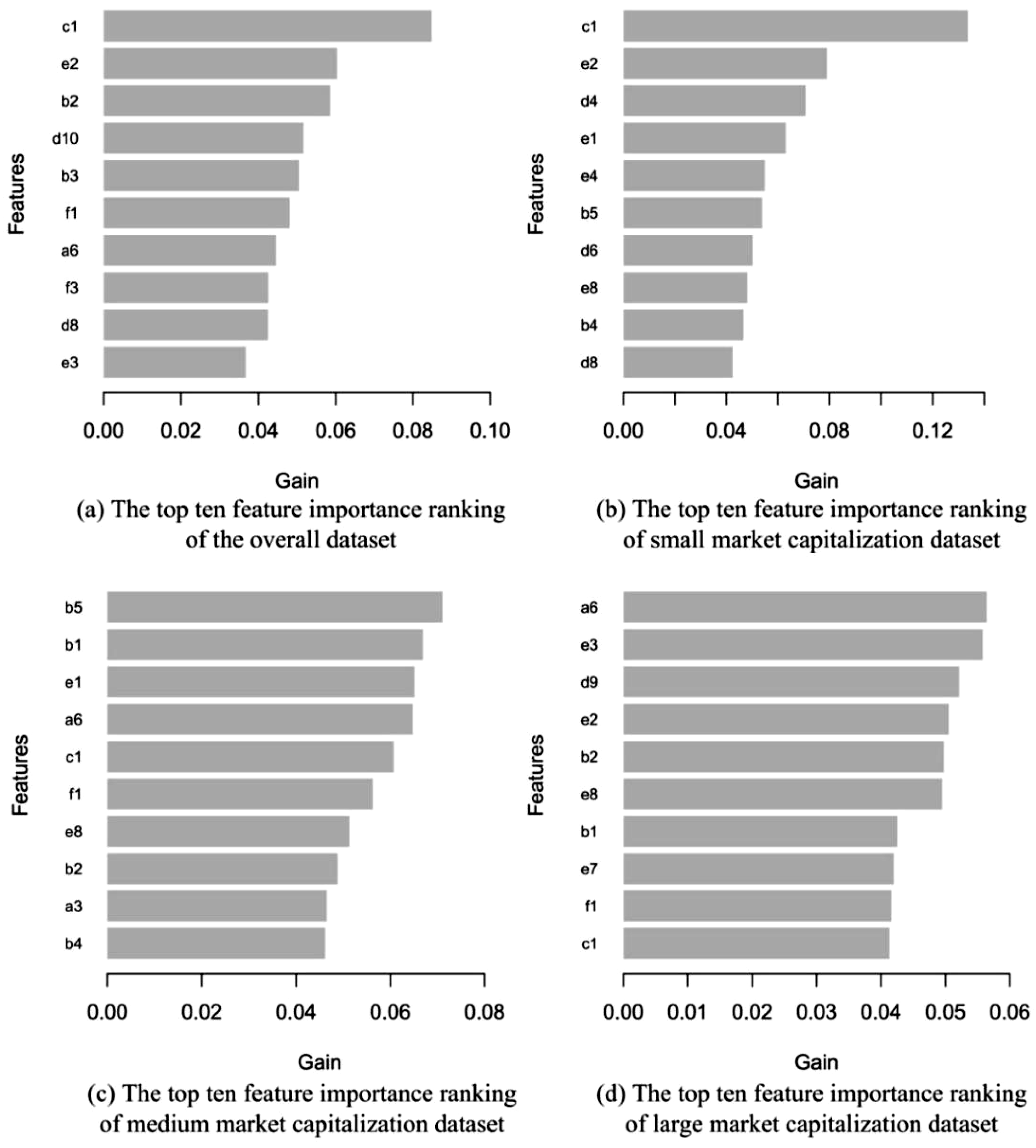
Figure 7.
SHAP values for each feature for prediction in the small-capitalization samples.

Figure 8.
SHAP dependence plots for the top four critical features for stock price crash prediction on the small-market capitalization samples.
Figure 8.
SHAP dependence plots for the top four critical features for stock price crash prediction on the small-market capitalization samples.

Table 1.
The financial indicators that are used as features for predicting the stock price crashes.
| Category | Codename | Features (Financial Indicator) |
|---|---|---|
| Debt-Paying Ability | a1 | Current Ratio |
| a2 | Quick Ratio | |
| a3 | Debt to Asset Ratio | |
| a4 | Equity Multiplier | |
| a5 | Debt to Equity Ratio | |
| a6 | Long-Term Debt to Asset Ratio | |
| Operating Capacity | b1 | Receivables Turnover Ratio |
| b2 | Inventory Turnover Ratio | |
| b3 | Operating Cycle | |
| b4 | Current Assets Turnover Ratio | |
| b5 | Fixed Assets Turnover Ratio | |
| b6 | Capital Intensity Rate | |
| b7 | Total Assets Turnover Ratio | |
| Growth Ability | c1 | Total Assets Growth Rate |
| c2 | Sustainable Growth Rate | |
| Profitability | d1 | Return on Assets Ratio |
| d2 | Return on Total Assets Ratio | |
| d3 | Return on Equity Ratio | |
| d4 | Gross Profit Margin Ratio | |
| d5 | Operating Expense Ratio | |
| d6 | Operating Profit Margin Ratio | |
| d7 | Net Profit Margin Ratio | |
| d8 | Expense to Sales Ratio | |
| d9 | Administration Expense Ratio | |
| d10 | Financial Expense Ratio | |
| Capital Structure | e1 | Current Assets to Total Assets Ratio |
| e2 | Cash to Assets Ratio | |
| e3 | Working Capital Over Total Assets Ratio | |
| e4 | Fixed Assets Ratio | |
| e5 | Shareholder Equity Ratio | |
| e6 | Current Liability Ratio | |
| e7 | Non-Current Liability Ratio | |
| e8 | Operating Profit Percentage | |
| Cash Flow | f1 | Operating Cash Flow to Sales Ratio |
| f2 | Net Operating Cash Flow to Sales Ratio | |
| f3 | Cash Return on Total Assets Ratio | |
| f4 | Cash Operating Index |
Table 2.
The value search range of the hyperparameters optimization for the XGBoost model.
| Hyperparameters | Brief Description | Value Search Range |
|---|---|---|
| eta | It controls the learning rate, and it can be used to prevent overfitting by making the boosting process more conservative. | 0.01~0.3 |
| max_depth | The maximum depth of a tree. | 3~10 |
| min_child_weight | The minimum sum of instance weight (Hessian) needed in a child. If the tree partition step results in a leaf node with a sum of instance weight less than it, the building process will give up further partitioning. | 0.5~6 |
| colsample_bytree | The subsample ratio of columns when constructing each tree. | 0.4~1 |
| gamma | The minimum loss reduction required to make a further partition on a leaf node of the tree. The larger the gamma, the more conservative the algorithm will be. | 0~5 |
| nrounds | The maximum number of boosting iterations. | 75~100 |
Table 3.
The confusion matrix for the out-of-sample prediction results.
| Positive Sample | Negative Sample | |
|---|---|---|
| Positive prediction | TP (True positive) | FP (False positive) |
| Negative prediction | FN (False negative) | TN (True negative) |
Table 4.
A list of the proposed method and benchmark methods.
| No | Methods | Description |
|---|---|---|
| 1 | XGBoost–NSGA-II–SHAP (proposed method) | It combines XGBoost, NSGA-II, and SHAP. XGBoost is used to predict stock price crashes; NSGA-II is used to optimize the hyperparameters of the XGBoost prediction method; SHAP is adopted to explain the prediction model. |
| 2 | XGBoost–GS | It integrates XGBoost and grid search (GS). XGBoost is used to predict the stock price crash, and GS is used to optimize the hyperparameters of the prediction model. |
| 3 | RF | A stock price crash prediction model based on a random forest (RF)-based method. |
| 4 | DT | A stock price crash prediction model based on a decision tree (DT)-based method. |
| 5 | SVM | A stock price crash prediction model based on the support vector machine (SVM)-based method. |
| 6 | ANN | A stock price crash prediction model based on the artificial neural network (ANN)-based method. |
Table 5.
A list of redundant features that were removed from each dataset.
| Category | Filtered Features Codes | Filtered Features |
|---|---|---|
| Whole dataset | a2, a4, b6, b7, d1, d5, d7, d9, e5, e7, f2 | Quick Ratio, Equity Multiplier, Capital Intensity Rate, Total Assets Turnover Ratio, Return on Assets Ratio, Operating Expense Ratio, Net Profit Margin Ratio, Administration Expense Ratio, Shareholder Equity Ratio, Non-Current Liability Ratio, Net Operating Cash Flow to Sales Ratio. |
| Small-Capitalization dataset | a2, a4, b3, b6, b7, d1, d5, d7, d9, d10, e3, e5, e7, f2 | Quick Ratio, Equity Multiplier, Operating Cycle, Capital Intensity Rate, Total Assets Turnover Ratio, Return on Assets Ratio, Operating Expense Ratio, Net Profit Margin Ratio, Administration Expense Ratio, Financial Expense Ratio, Working Capital Over Total Assets Ratio, Shareholder Equity Ratio, Non-Current Liability Ratio, Net Operating Cash Flow to Sales Ratio. |
| Medium- Capitalization dataset | a2, a4, b3, b6, b7, d1, d3, d5, d6, d7, d10, e5, e7, f2 | Quick Ratio, Equity Multiplier, Operating Cycle, Capital Intensity Rate, Total Assets Turnover Ratio, Return on Assets Ratio, Return on Equity Ratio, Operating Expense Ratio, Operating Profit Margin Ratio, Net Profit Margin Ratio, Financial Expense Ratio, Shareholder Equity Ratio, Non-Current Liability Ratio, Net Operating Cash Flow to Sales Ratio. |
| Large- Capitalization dataset | a2, a4, b6, d1, d3, d5, d6, d7, d10, e5, e6 | Quick Ratio, Equity Multiplier, Capital Intensity Rate, Return on Assets Ratio, Return on Equity Ratio, Operating Expense Ratio, Operating Profit Margin Ratio, Net Profit Margin Ratio, Financial Expense Ratio, Shareholder Equity Ratio, Current Liability Ratio. |
Table 6.
Results of stock price crash prediction for the proposed method and benchmark methods.
| Method | SVM | RF | ANN | DT | XGBoost–GS | XGBoost–NSGA-II |
|---|---|---|---|---|---|---|
| Panel A. Stock samples of small market capitalization | ||||||
| ACC | 63.31% | 64.24% | 55.90% | 62.25% | 59.60% | 78.41% |
| TPR | 85.88% | 82.35% | 58.43% | 69.12% | 54.12% | 81.31% |
| FPR | 59.52% | 50.60% | 47.22% | 43.37% | 33.33% | 26.09% |
| PPV | 59.35% | 57.14% | 60.47% | 56.62% | 67.65% | 82.86% |
| Panel B. Stock samples of medium market capitalization | ||||||
| ACC | 50.67% | 57.04% | 50.33% | 61.96% | 62.67% | 73.83% |
| TPR | 47.59% | 55.71% | 69.01% | 59.74% | 61.33% | 75.90% |
| FPR | 46.34% | 41.67% | 66.67% | 36.05% | 35.82% | 28.09% |
| PPV | 45.71% | 56.52% | 48.51% | 59.74% | 65.71% | 71.59% |
| Panel C. Stock samples of large market capitalization | ||||||
| ACC | 52.84% | 54.03% | 49.54% | 58.82% | 48.63% | 63.93% |
| TPR | 35.54% | 39.60% | 45.54% | 50.47% | 48.15% | 60.81% |
| FPR | 31.97% | 32.73% | 46.96% | 34.35% | 50.00% | 31.25% |
| PPV | 49.35% | 52.63% | 46.00% | 54.55% | 73.39% | 75.00% |
| Panel D. Whole stock samples | ||||||
| ACC | 55.30% | 57.17% | 55.13% | 58.08% | 57.34% | 62.88% |
| TPR | 53.61% | 59.86% | 49.26% | 62.33% | 58.92% | 63.40% |
| FPR | 43.20% | 45.45% | 38.58% | 46.49% | 44.29% | 37.86% |
| PPV | 52.61% | 56.17% | 57.76% | 59.09% | 57.76% | 70.51% |
Table 7.
Results of the proposed XGBoost–NSGA-II method for stock price crash prediction on four different datasets.
Table 7.
Results of the proposed XGBoost–NSGA-II method for stock price crash prediction on four different datasets.
| Category | ACC | TPR | FPR | PPV |
|---|---|---|---|---|
| Small-capitalization dataset | 78.41% | 81.31% | 26.09% | 82.86% |
| Medium-capitalization dataset | 73.83% | 75.90% | 28.09% | 71.59% |
| Large-capitalization dataset | 63.93% | 60.81% | 31.25% | 75.00% |
| Whole dataset | 62.88% | 63.40% | 37.86% | 70.51% |
Publisher’s Note: MDPI stays neutral with regard to jurisdictional claims in published maps and institutional affiliations. |
© 2022 by the authors. Licensee MDPI, Basel, Switzerland. This article is an open access article distributed under the terms and conditions of the Creative Commons Attribution (CC BY) license (https://creativecommons.org/licenses/by/4.0/).
Share and Cite
MDPI and ACS Style
Deng, S.; Zhu, Y.; Duan, S.; Fu, Z.; Liu, Z. Stock Price Crash Warning in the Chinese Security Market Using a Machine Learning-Based Method and Financial Indicators. Systems 2022, 10, 108. https://doi.org/10.3390/systems10040108
AMA Style
Deng S, Zhu Y, Duan S, Fu Z, Liu Z. Stock Price Crash Warning in the Chinese Security Market Using a Machine Learning-Based Method and Financial Indicators. Systems. 2022; 10(4):108. https://doi.org/10.3390/systems10040108
Chicago/Turabian StyleDeng, Shangkun, Yingke Zhu, Shuangyang Duan, Zhe Fu, and Zonghua Liu. 2022. "Stock Price Crash Warning in the Chinese Security Market Using a Machine Learning-Based Method and Financial Indicators" Systems 10, no. 4: 108. https://doi.org/10.3390/systems10040108
Note that from the first issue of 2016, this journal uses article numbers instead of page numbers. See further details here.