Abstract
Systemic racism, which exists when minorities experience harmful outcomes from implicit or explicit bias, has recently been a much-discussed phenomenon. Systemic racism may exist, even though explicit bias is mostly illegal, because of structures of policy or behavior that generate deleterious outcomes. Bank financing for housing purchase or improvement is one such structure. An overtly discriminatory policy facilitated by an agency of the United States government, “redlining” on “residential security maps” depicted supposedly high-risk lending areas in red. These historical maps have led to low housing values today in formerly redlined areas. Even though the practice has been illegal for decades, traditional lenders nowadays decline loans in those areas because they are too small to be profitable. A system dynamics model shows the systemic structure of this situation. The model simulates various policies for its solution. Robust (but expensive) policies involve subsidies to lenders or lending from governments or nonprofits. Less robust but potentially cheaper policy would require lenders to make small loans anyway. Any of these policies would help break the adverse reinforcing loop of declining housing, inability to borrow to improve the housing, and further housing decline.
1. Introduction
Systemic racism, a situation under which members of minority races experience deleterious outcomes such as higher arrest rates or greater wealth inequalities, stemming from explicit or implicit bias, has been widely discussed in recent years. Even though explicit bias has been illegal since the 1960s, structures of policy or behavior that generate unnecessarily lopsided outcomes create systemic racism. The present paper will examine one such systemic structure—bank financing of housing purchase or improvement [1].
“Redlining” was an overtly discriminatory policy facilitated by a federal agency of the United States government, the Home Owners’ Loan Corporation (HOLC), founded in 1933 as part of the New Deal [2]. The HOLC commissioned “residential security maps” for scores of cities across the country. The term “redlining” came from how the maps used four colors to depict neighborhoods as belonging to four categories of loan risk:
- Best (green).
- Desirable (blue).
- Declining (yellow).
- Hazardous (red).
See, for example, the residential security map for Detroit in Figure 1.
The U.S. federal government encouraged state and local governments and private companies, especially banks, to use these maps to deny goods and services, including mortgage and home-improvement loans, to citizens or customers living in the areas depicted in red. The passage of the Fair Housing Act of 1968 outlawed redlining [3]. However, in a good example of what the system dynamics community recognizes as a chronic problem caused by an underlying systemic structure, the consistent application of redlining from the 1920s through the 1960s created conditions that have allowed racial differences in housing lending to persist [4].
There is significant overlap between Detroit’s 1939 redlined areas and areas of Detroit that suffered shallower recoveries from the Great Recession of 2007–2009 [5]. Numerous recent academic studies have rigorously examined this issue (see, for example, [6,7,8,9,10]) and found that it exists. However, scholars or practitioners have offered few policy or practice responses or interventions that could be implemented in specific cities or regions.
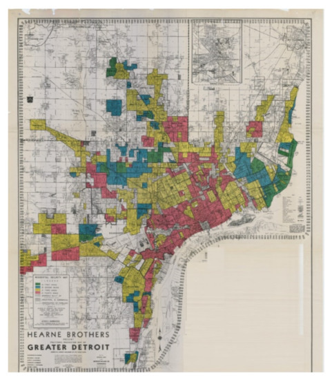
Figure 1.
“Residential Security Map” for Detroit, 1939. Source: [11].
A journalistic account by Eisen [12] sparked my interest in this topic. He described how Detroit, with 700,000 residents, originated only about 1700 mortgages in 2019 while having a larger number of tax foreclosures. As Eisen puts it:
“…Making mortgages in Detroit is a convoluted task. The dearth of credit is largely a consequence of battered property values plus a commercial reality that depresses them further: Lenders can’t earn money on tiny mortgages, so they don’t make them.”.[11]
Eisen’s statement concisely captures the paradoxical legacy of redlining: even though it is illegal, redlining in the past has led to diminished property values today, which makes getting a loan very difficult because lenders find small loans unprofitable. Even if lenders use transparent lending standards that do not explicitly discriminate against minority loan applicants, the history of redlining makes lending to them unprofitable and impracticable.
2. Materials and Methods
2.1. Dynamic Hypothesis
The causal loop diagram in Figure 2 captures the dynamic hypothesis showing this deleterious systemic structure. The hypothesis has two reinforcing loops, with important non-linear relationships governing each of them.
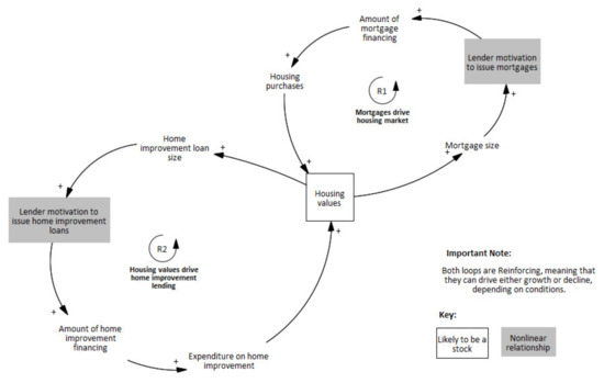
Figure 2.
Causal loop diagram showing the systemic structure of the legacy of redlining. Source [1].
Reinforcing loop 1, “Mortgages drive housing market”, captures the basic point that as houses come on the market, prospective purchasers apply for mortgages based on the negotiated price. If the mortgage is above the lender’s cost threshold, and if the applicant passes financial muster, the loan is issued, the applicant purchases the house, and the process repeats when the house next goes on sale. A reinforcing loop such as this one should drive pricing growth in the market.
Reinforcing loop 2, “Housing values drive home improvement lending”, does the same sort of thing, only for loans designed to improve (as opposed to purchase) existing homes. In the same way as loop R1, this loop should drive up the value of homes.
However, reinforcing loops can, if they proceed in the “wrong” direction, lead to decreases in value. In a paper examining low-income neighborhoods, but without an explicit systems perspective, Swanstrom [13] noted this phenomenon.
This is where the two non-linear variables in the causal loop diagram, lender motivations, play a crucial role. If the amount of the mortgage or home improvement loan is too small, the lender’s transparent lending standards will lead it to deny the loan. If “Mortgage size” or “Home improvement loan size” reduce, as they have in historically redlined neighborhoods, then “Lender motivation” drops, cutting off the loans that drive value, and the loops drive value into decline.
Much recent work in operations research has focused on “community-engaged OR” [14] and “community operational research” [15]. These approaches recommend multiple methods, and so the study reported here, using both qualitative and quantitative system dynamics, is aligned with the notion of using multiple operations research methods to examine difficult urban problems.
2.2. Stock and Flow Model
Figure 3 shows a stock-and-flow model (see Appendix A for a full listing of the model’s equations) that attempts to capture the dynamic hypothesis. Please note that this is a stylized model. It does not attempt to replicate any specific U.S. city; it merely attempts to show the relationship among the variables as depicted in the dynamic hypothesis.
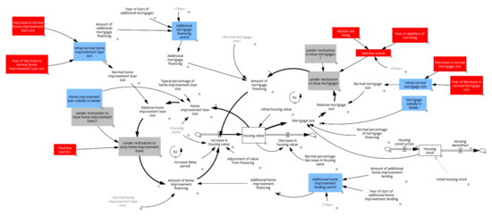
Figure 3.
Stock and flow model of redlining issue. Source [1].
Housing value drives both mortgage lending and home-improvement lending, as shown by the bold arrows of loops R1 and R2, respectively. However, the lenders will not lend unless the relative size of the loan is large enough to motivate them to do so. Non-linear functions, shown in Figure 4, govern the motivation to lend either mortgages or home-improvement loans. As shown in Figure 3, the input to these functions is the ratio of the loan size requested to the “normal” loan size. If that ratio is 0.8 or less, the motivation to lend is ten percent or less. Only when the ratio of the requested loan is above 0.8 is there substantial motivation to lend.
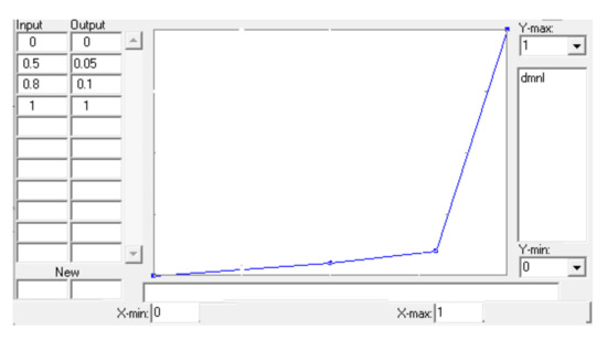
Figure 4.
Nonlinear functions governing motivation to lend. Source [1].
The model assumes that either kind of loan will modify Home value, with some adjustment constants: eighty percent for mortgages and seventy-five percent for home-improvement loans. The model also assumes that modifications in home value are not instantaneous; there is a third order delay in the change in home value for any given adjusted loan amount.
The model runs from the years 1950 to 2020, so somehow the effect of redlining needed to be in the model. The model contains a redline switch (shown in red in Figure 3) that allows for the zeroing of the linear functions. That is, while redlining is in effect, Lender motivation for either mortgages or home-improvement loans is zero. The formulation of the switch allows the modeler to turn redlining off in any year.
Lastly, the model contains some variables that allow policy simulation: changes in initial normal loan values (to test whether motivation to lend small amounts would improve with lower “normal” loan targets) and variables that allow us to test for what would happen if government agencies or nonprofit organizations set up programs to lend money outside the traditional lending system of banks and mortgage companies. Figure 3 shows these variables in blue.
3. Results
3.1. Model Test: Redlining for Entire Period (or No Redlining Ever)
Figure 5 shows the result one would expect were redlining to persist from 1950 to 2020—a steady decline in housing values. In contrast, were redlining abolished in 1950, the beginning of the period, there would be steady growth in housing values, as Figure 6 depicts.
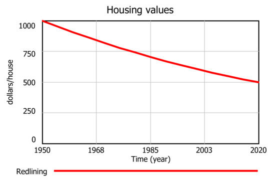
Figure 5.
Housing values with persistent redlining. Source [1].
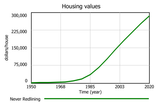
Figure 6.
Redlining abolished 1950. Source [1].
Model Validation
Historical data on housing prices (especially data covering 1950 to 2020) are surprisingly difficult to find. However, more recent data support the validity of the model. Figure 7 shows mean home sales prices from 2005 through 2015 for Detroit, Wayne County (the metropolitan area around Detroit) and the entire United States. The reader can see that the curve for home prices in the city of Detroit (the dark blue curve) is declining and low, similar to the curve shown in Figure 5.
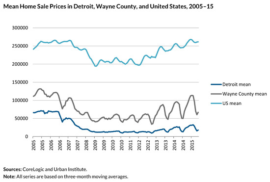
Figure 7.
Home prices Detroit, Wayne County, Michigan and United States. Source [16]. Permission is granted for reproduction with attribution to the Urban Institute.
3.2. Policy Experiments
As mentioned earlier, many papers in the literature have covered the existence of persistent effects of redlining, but few offer potentially effective policy solutions for the specific problem of low levels of bank lending. For example, Coffin [17] suggested using Tax Increment Financing (TIF) to make progress on this problem, but her suggestion was more appropriate for supporting developers of large housing projects. Kang [18] suggests reparations and “restorative justice”, neither of which address the issue of current bank lending policies. Reece [19] points out that adopting a racial equity lens is a prerequisite for ameliorative action in this domain. Long-term redlining led to depressed property values, which makes these neighborhoods attractive targets for gentrification, continuing to shut out the lower-income people who are the focus of the present paper. McGrew [20] suggests “homeownership” as a solution to historic racial discrimination in housing, and offers a form of reparations that would “take the form of the dissemination of land or subsidies to buy land whereby African Americans would be given a preference in homeownership funding”. This policy recommendation is similar to the policy of subsidizing lenders, tested later, so McGrew’s is an exception to the critique of a low number of policy recommendations.
We turn now to a few potential policies for improvement. Please note that these policies were not derived from prior research; instead, they were suggested by the systemic structure of this problem, where financing for individual homeowners (or potential homeowners) is more germane.
3.2.1. Scenario 1: Redlining Abolished Late in Period
Even though the federal government formally abolished redlining in 1968, it appears that lenders did not necessarily begin to stop the practice at that time. Figure 8 shows what would happen were lenders to have stopped de facto redlining in either 2000 or 2010. As is often the case with systems, given their nonlinear nature, the earlier the better. Discontinuation of redlining in 2000 would have begun the growth curve much more effectively than doing so even only ten years later. However, the gains in housing value in either of these scenarios are modest, to say the least. From a cost/benefit standpoint, this policy appears at first glance to be good—there is no explicit expense (no government subsidies, or foregone profits, for example) and some gain. Still, neither of these scenarios is realistic, since, as Eisen [11] related, explicit change in public policy did not lead to increases in housing value or lending. I include them to show the workings of the model.
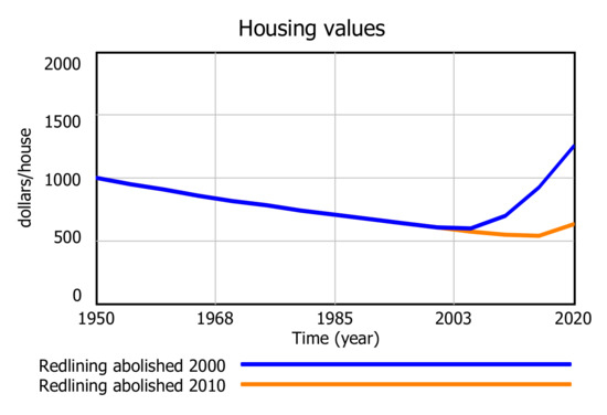
Figure 8.
Redlining abolished late in period. Source [1].
3.2.2. Scenario 2: Subsidizing Lenders
Since the problem is that loan sizes are too small to motivate lending, one possible policy would be for the government or nonprofit agencies to subsidize mortgages or home-improvement loans, making payments directly to lenders so that the loan amounts would surpass the threshold for granting the loan. Figure 9 shows the effects of subsidizing loan amounts by doubling their indicated size.
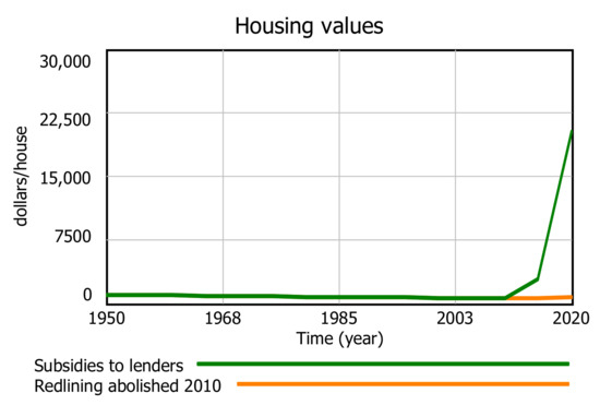
Figure 9.
Double subsidies to lenders. Source [1].
Figure 8 showed that abolishing de facto redlining in 2010 had a modest effect on housing value. Figure 9 shows that supplementing that policy with one that subsidizes lenders (for both kinds of loans) with double the amount of the loan results in substantially higher improvements in housing value. Figure 10 shows that subsidies even half that size are somewhat robust at improving housing values.
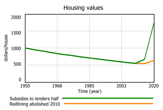
Figure 10.
Half subsidies to lenders. Source [1].
Either level of subsidy would be expensive, as the subsidies could range from USD 5000 to USD 10,000 for mortgages and USD 2500 to USD 5000 for home-improvement loans. However, the benefits could outweigh these costs, as properties increase in value from the initial USD 1000 up to USD 20,000. As housing quality improves, there is every reason to believe that overall quality of the neighborhoods involved would improve. Furthermore, it is possible that over time, as housing values increase, local governments might recoup some of this expense from increased property taxes.
3.2.3. Scenario 3: Direct Lending from Government or Nonprofits
Another policy would be to have governments or nonprofits with lower or no profit motive lend directly to prospective or current homeowners, even when the loans are small. Figure 11 shows the result of this policy, which ended redlining in 2010, and adds, starting that year, USD 1000 in additional lending for mortgages and USD 500 for home-improvement loans.
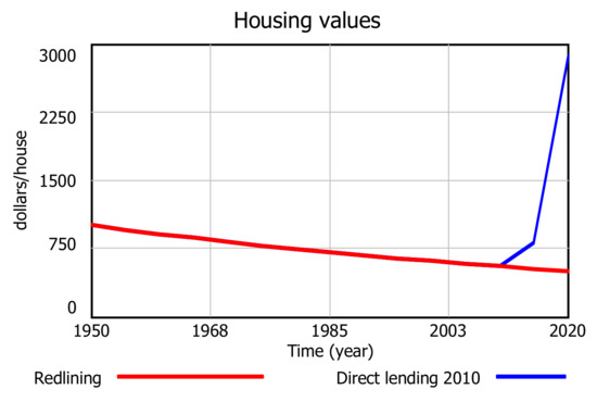
Figure 11.
Direct lending to homeowners from government or nonprofits. Source [1].
While this does not appear to be as potent as increasing the motivation of traditional lenders, it could be a less expensive and more feasible approach. Borrowers would still get the small loans they need and the agencies or nonprofits would get repayments that could make this approach self-sustaining.
3.2.4. Scenario 4: Requiring Lenders to Make Smaller Loans
Some jurisdictions require lenders to make small loans, at least for some percentage of their portfolios. Figure 12 shows the effects of a policy where, starting in 2010, policymakers require lenders to make smaller mortgages and home-improvement loans. The effect is modest, and would hurt lenders, who would likely lose money on each loan. However, they should be able to claim the losses against their tax liability. Over time, a modest approach such as this might succeed in breaking the cycle of homeowners or prospective homeowners’ being unable to improve their actual or prospective housing, ultimately raising property values in a given neighborhood. Given the losses to lenders, though, it is difficult to see how this could be a large-scale approach.
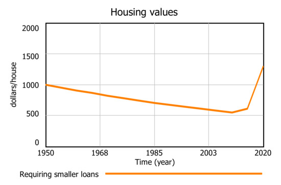
Figure 12.
Requiring lenders to make smaller loans. Source [1].
Table 1 shows the parameter settings for the four policy tests.

Table 1.
Parameter settings for policy tests. Source [1].
3.2.5. Comparison of Policies
Figure 13 compares the four suggested policies. The abolition of redlining in 2010, by itself, has begun to ameliorate the problem, but quite slowly. Adding half subsidies to lenders is more potent, but would require large sums to motivate the lenders to lend. The third policy tested, adding direct lending to homeowners or prospective homeowners, was the most potent of the three policies, and had the added benefit of being financially reasonable and potentially sustainable. The fourth policy, requiring lenders to make smaller loans, was effective, but not as much as subsidizing lenders and having government or nonprofits make direct loans to actual or prospective homeowners. However, this policy is the least scalable, as it would involve too much loss for the lenders. Direct lending of small loans by nonprofits or government would be the most scalable and highest leverage of the policies examined in this paper. Table 2 shows a breakdown of the financial and social costs and benefits.
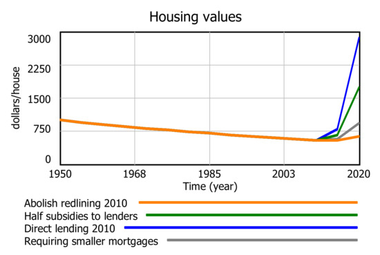
Figure 13.
Comparison of policy results. Source [1].

Table 2.
Costs and benefits of policies.
4. Discussion
Many studies have shown that homeowning is source of wealth and that differences in homeownership are partly responsible for the gap in wealth among racial groups (see, for example, [16,21]). As several previously cited papers showed, a “systemic structure” created by prior racial discrimination is responsible for lower homeownership, and therefore, lower wealth, in some places today.
The present paper does not reveal any profoundly innovative solutions, but it does illuminate the systemic nature of the problem. A term frequently used in the housing industry is “pride of ownership”. Many people living in formerly redlined areas strive to purchase and improve the homes in which they live or want to live. For example, one Detroit resident highlighted in Eisen [11] purchased two houses for a total of USD 3300 and then spent USD 100,000 of his own savings to upgrade them for his and his mother’s habitation.
However, many people in these circumstances cannot “break the cycle”, familiar as a perverse reinforcing loop to most systems thinkers, of declining housing, inability to get credit to improve the housing, further housing decline, etc. Despite its flaws and limitations, the model interrogated in the present paper shows that this issue is potentially amenable to solution and helps move the conversation forward.
Funding
This research received no external funding.
Institutional Review Board Statement
Not applicable.
Informed Consent Statement
Not applicable.
Data Availability Statement
Not applicable.
Conflicts of Interest
The author declares no conflict of interest.
Appendix A. The Model in Text Form
The model used in this article, shown graphically in Figure 7, was formulated using the Vensim system dynamics program. Here is a text version of all the model’s variables, constants and parameters.
| Normal home improvement loan size = initial normal home improvement loan size |
| Units: dollars/house |
| Decrease in normal home improvement loan size = 2250 |
| Units: dollars/house |
| Initial normal home improvement loan size = 2500-STEP (decrease in normal home improvement loan size; year of decrease in normal home improvement loan size) |
| Units: dollars/house |
| Year of decrease in normal home improvement loan size = 2021 |
| Units: year |
| Initial normal mortgage size = 10,000-STEP (decrease in normal mortgage size; year of decrease in normal mortgage size) |
| Units: dollars/house |
| Year of decrease in normal mortgage size = 2021 |
| Units: year |
| Decrease in normal mortgage size = 9500 |
| Units: dollars/house |
| Normal mortgage size = initial normal mortgage size |
| Units: dollars/house |
| Mortgage size = (housing value * normal percentage of mortgage financing) + mortgage subsidy to lender |
| Units: dollars/house |
| Home improvement loan size = (typical percentage of home improvement loan size * housing value) + home improvement loan subsidy to lender |
| Units: dollars/house |
| Home improvement loan subsidy to lender = 0 |
| Units: dollars/house |
| Relative home improvement loan size = home improvement loan size/normal home improvement loan size |
| Units: dimensionless |
| Mortgage subsidy to lender = 0 |
| Units: dollars/house |
| Year of start of additional mortgages = 2021 |
| Units: year |
| Additional home improvement financing = 0 + additional home improvement lending switch |
| Units: dollars/house |
| Additional home improvement lending switch = IF THEN ELSE (time < year of start of additional home improvement lending, 0—amount of additional home improvement lending) |
| Units: dollars/house |
| Additional mortgage financing = additional mortgage financing switch |
| Units: dollars/house |
| Additional mortgage financing switch = IF THEN ELSE (time < year of start of additional mortgages, 0—amount of additional mortgage financing) |
| Units: dollars/house |
| Amount of mortgage financing = (normal mortgage size * lender motivation to issue mortgages) + additional mortgage financing |
| Units: dollars/house |
| Amount of additional home improvement lending = 0 |
| Units: dollars/house |
| Amount of additional mortgage financing = 0 |
| Units: dollars/house |
| Amount of home improvement financing = (normal home improvement loan size * lender motivation to issue home-improvement loans) + additional home improvement financing |
| Units: dollars/house |
| Increase in housing value = DELAY3 ((amount of home improvement financing + amount of mortgage financing) * adjustment of value from financing, increased delay period) |
| Units: dollars/house/year |
| Increase delay period = 10 |
| Units: year |
| Year of start of additional home improvement lending = 2021 |
| Units: year |
| Abolish redlining = 1 |
| Units: dimensionless |
| Comment: Setting this to 1 makes redlining illegal. |
| Lender motivation to issue home-improvement loans = lender motivation to issue home-improvement loans f(relative home improvement loan size) * redline switch |
| Units: dimensionless |
| Lender motivation to issue mortgages = lender motivation to issue mortgages f(relative mortgage size) * redline switch |
| Units: dimensionless |
| Normal percentage of mortgage financing = 0.8 |
| Units: dimensionless |
| Red line switch = IF THEN ELSE (time < year of abolition of redlining, 0—abolish redlining) |
| Units: dimensionless |
| Comment: set to zero to implement “red line” lending policy. This zeroes out the motivation to lend. |
| Year of abolition of redlining = 2021 |
| Units: year |
| Adjustment of value from financing = 0.75 |
| Units: dimensionless/year |
| Units: financing does not increase value one-for-one. This makes an arbitrary adjustment. |
| Normal percentage decrease in housing value = 0.01 |
| Units: dimensionless/year |
| Decrease in housing value = housing value * normal percentage decrease in housing value |
| Units: dollars/(year * house) |
| Typical percentage of home improvement loan size = 0.8 |
| Units: dimensionless |
| Housing value = INTEG (increase in housing value—decrease in housing value; initial housing value) |
| Units: dollars/house |
| Lender motivation to issue home-improvement loans f([(0, 0)–(1, 1)], (0, 0), (0.5, 0.05), (0.8, 0.1), (1, 1)) |
| Units: dimensionless |
| Comment: ascending non-linear function; as loan size increases, motivation to lend increases. |
| Lender motivation to issue mortgages f([(0, 0)–(1, 1)], (0, 0), (0.5, 0.05), (0.8, 0.1), (1, 1)) |
| Units: dimensionless |
| Comment: ascending non-linear function; as loan size increases, motivation to lend increases. |
| Relative mortgage size = mortgage size/normal mortgage size |
| Units: dimensionless |
| Initial housing value = 1000 |
| Units: dollars/house |
| ******************************************************** |
| Control |
| ******************************************************** |
| Units: simulation control parameters |
| FINAL TIME = 2020 |
| Units: year |
| Units: the final time for the simulation. |
| INITIAL TIME = 1950 |
| Units: year |
| Units: the initial time for the simulation. |
| SAVEPER = 5 |
| Units: year |
| Units: the frequency with which output is stored. |
| TIME STEP = 0.25 |
| Units: year |
| Units: the time step for the simulation. |
References
- Voyer, J. Housing finance: A vestige of systemic racism? In Proceedings of the 39th International Conference of the System Dynamics Society, Chicago, IL, USA, 25–29 July 2021. [Google Scholar]
- National Archives of the United States. Records of the Home Owners’ Loan Corporation (HOLC), 1933–1951. Available online: https://www.archives.gov/research/guide-fed-records/groups/195.html#195.3 (accessed on 13 March 2021).
- Department of Housing and Urban Development. History of Fair Housing. 2021. Available online: https://www.hud.gov/program_offices/fair_housing_equal_opp/aboutfheo/history (accessed on 13 March 2021).
- Jan, T. Redlining was banned 50 years ago. It’s still hurting minorities today. The Washington Post. 28 March 2018. Available online: https://www.washingtonpost.com/news/wonk/wp/2018/03/28/redlining-was-banned-50-years-ago-its-still-hurting-minorities-today/ (accessed on 13 March 2021).
- McClure, L. Map: Redlining and Health in Detroit. DETROITography, 2008. Available online: https://detroitography.com/2020/02/17/map-redlining-and-health-in-detroit-2008/ (accessed on 13 March 2021).
- Mehdipanah, R.; Bess, K.; Tomkowiak, S.; Richardson, A.; Stokes, C.; White Perkins, D.; Cleage, S.; Israel, B.A.; Schulz, A.J. Residential Racial and Socioeconomic Segregation as Predictors of Housing Discrimination in Detroit Metropolitan Area. Sustainability 2020, 12, 10429. [Google Scholar] [CrossRef]
- McClure, E.; Feinstein, L.; Cordoba, E.; Douglas, C.; Emch, M.; Robinson, W.; Galea, S.; Aiello, A.E. The legacy of redlining in the effect of foreclosures on Detroit residents’ self-rated health. Health Place 2019, 55, 9–19. [Google Scholar] [CrossRef] [PubMed]
- Mitchell, B.; Franco, J. HOLC “Redlining” Maps: The Persistent Structure of Segregation and Economic Inequality. Report of National Community Reinvestment Coalition. 2018. Available online: https://ncrc.org/holc/ (accessed on 13 March 2021).
- Nardone, A.; Chiang, J.; Corburn, J. Historic Redlining and Urban Health Today in U.S. Cities. Environ. Justice 2020, 13, 109–119. [Google Scholar] [CrossRef]
- Silverman, R.M. Redlining in a Majority Black City? Mortgage Lending and the Racial Composition of Detroit Neighborhoods. West. J. Black Stud. 2005, 29, 531–541. [Google Scholar]
- Hill, A.B. Detroit Redlining Map, 1939. DETROITography, 2014. Available online: https://detroitography.com/2014/12/10/detroit-redlining-map-1939/ (accessed on 13 March 2021).
- Eisen, B. Dearth of Credit Starves Detroit’s Housing Market. Wall Street Journal. 29 October 2020. Available online: https://library.umaine.edu/auth/EZproxy/test/authej.asp?url=https://search.proquest.com/newspapers/dearth-credit-starves-detroit-s-housing-market/docview/2455565459/se-2?accountid=8120 (accessed on 13 March 2021).
- Swanstrom, T. Market-savvy housing and community development policy: Grappling with the equity-efficiency trade-off. In Facing Segregation: Housing Policy Solutions for a Stronger Society; Metzger, M.W., Webber, H.S., Eds.; Oxford University Press: New York, NY, USA, 2019; pp. 173–196. [Google Scholar]
- Midgley, G.; Johnson, M.P.; Chichirau, G. What is community operational research? Eur. J. Oper. Res. 2018, 268, 771–783. [Google Scholar] [CrossRef]
- Johnson, M.P.; Midgley, G.; Chichirau, G. Emerging trends and new frontiers in community operational research. Eur. J. Oper. Res. 2018, 268, 1178–1191. [Google Scholar] [CrossRef]
- Poethig, E.C.; Schilling, J.; Goodman, L.; Bai, B.; Gastner, J.; Pendall, R.; Fazili, S. The Detroit Housing Market: Challenges and Innovations for a Path Forward. Urban Institute Research Report. 2017. Available online: https://www.urban.org/sites/default/files/publication/88656/detroit_path_forward_0.pdf (accessed on 9 February 2022).
- Coffin, S.L. Financing affordability: Tax increment financing and the potential for concentrated reinvestment. In Facing Segregation: Housing Policy Solutions for a Stronger Society; Metzger, M.W., Webber, H.S., Eds.; Oxford University Press: New York, NY, USA, 2019; pp. 197–214. [Google Scholar]
- Kang, H.H. Looking Toward Restorative Justice for Redlined Communities Displaced by Eco-Gentrification. Mich. J. Race Law 2021, 23, 26. [Google Scholar] [CrossRef]
- Reece, J. Confronting the Legacy of “Separate but Equal”: Can the History of Race, Real Estate, and Discrimination Engage and Inform Contemporary Policy? RSF Russell Sage Found. J. Soc. Sci. 2021, 7, 110–133. [Google Scholar] [CrossRef]
- McGrew, T. The History of Residential Segregation in the United States, Title VIII, and the Homeownership Remedy. Am. J. Econ. Sociol. 2018, 77, 1013–1048. [Google Scholar] [CrossRef]
- Bhutta, N.; Chang, A.C.; Lisa, J.; Dettling, L.J.; Hsu, J.W.; Hewitt, J. Disparities in Wealth by Race and Ethnicity in the 2019 Survey of Consumer Finances. FEDS Notes; 2020. Available online: https://www.federalreserve.gov/econres/notes/feds-notes/disparities-in-wealth-by-race-and-ethnicity-in-the-2019-survey-of-consumer-finances-20200928.htm (accessed on 17 March 2021).
Publisher’s Note: MDPI stays neutral with regard to jurisdictional claims in published maps and institutional affiliations. |
© 2022 by the author. Licensee MDPI, Basel, Switzerland. This article is an open access article distributed under the terms and conditions of the Creative Commons Attribution (CC BY) license (https://creativecommons.org/licenses/by/4.0/).