Charging Station Planning for Electric Vehicles

Abstract

Charging station (CS) planning for electric vehicles (EVs) for a region has become an important concern for urban planners and the public alike to improve the adoption of EVs. Two major problems comprising this research area are: (i) the EV charging station placement (EVCSP) problem, and (ii) the CS need estimation problem for a region. In this work, different explainable solutions based on machine learning (ML) and simulation were investigated by incorporating quantitative and qualitative metrics. The solutions were compared with traditional approaches using a real CS area of Austin and a greenfield area of Bengaluru. For EVCSP, a different class of clustering solutions, i.e., mean-based, density-based, spectrum- or eigenvalues-based, and Gaussian distribution were evaluated. Different perspectives, such as the urban planner perspective, i.e., the clustering efficiency, and the EV owner perspective, i.e., an acceptable distance to the nearest CS, were considered. For the CS need estimation, ML solutions based on quadratic regression and simulations were evaluated. Using our CS planning methods urban planners can make better CS placement decisions and can estimate CS needs for the present and the future.

1. Introduction

Electric Vehicles (EVs) have become prominent these days as a result of their eco-friendliness and cost-saving characteristics [1,2]. Widespread adoption of electric vehicles (EVs) depends on the optimal placement of charging stations (CSs) [3]. In recent years, the need to place CSs efficiently and plan CS needs for a region has turned into an important concern for urban planners and the public alike. Moreover, it has been found that service providers prefer clustering instead of separation in the EV charging market [4]. Therefore, the electric vehicle charging station placement (EVCSP) problem, which tries to identify a CS for each EV such that the total distance traveled by EV owners for charging at the nearest CS is minimized, and tries to determine the CS need estimation for a region, have become two major research problems of EV charging station planning [3,5,6,7].

EVCSP solutions try to reduce the distance that the EV will travel to access the charging station and this impacts the state of the charge (SoC) of the electric vehicle [8]. Moreover, the proper location of the CS reduces the total expected cost of the charging process and increases the EV owner’s convenience [9]. A good CS need estimation for a region improves the customer satisfaction-involved operational cost, while considering the potential uncertainties [10].

In previous studies, EVCSP solutions have been developed by focusing on any one system based on a clustering method [11,12] or Geographical Information System (GIS) [13] or market survey, which often focus on spatial relationships to identify prime locations for CSs. Moreover, these methods have not been evaluated either quantitatively or qualitatively for a single planning area. In addition to this, the current CS needs estimators are based on weird adjustment factors and these estimations are also unexplainable [14,15]. Furthermore, these estimators have not considered future estimates of CS needs for the planning areas and they have not involved increasing EV penetration in these estimates.

In the majority of EVCSP solutions, the evaluation has been done predominantly using a single metric like the EV distance to the nearest CS, i.e., from an EV user’s perspective but not from a clustering efficiency perspective, i.e., urban planners or policy makers. Multiple metrics, i.e., (a) CS placement metrics and (b) clustering metrics, have been considered for EVCSP to evaluate if the clustering is good or not from a clustering perspective and an EV owners perspective, i.e., an acceptable distance to the nearest CS. These EVCSP metrics are explained in Section 2.2.

In our work, quantitative and qualitative metrics have been involved to investigate optimal CS placements and aid in decision making. Different perspectives, such as the clustering efficiency from an urban planner perspective, and an EV owners perspective, i.e., an acceptable distance to the nearest CS, provide multiple results with trade-offs. These results can be used to guide urban planners in making better CS placement approval decisions when many CSs (in the order of hundreds or more) need to be placed for charging at different locations of a planning area in an efficient manner, i.e., considering the clustering efficiency, the EV owners convenience, and the visual analysis of the system. Using our CS need estimation methods urban planners can estimate the CS need range, i.e., minimalist need, actual need, and future need, to take an appropriate decision on the CSs required in a planning area. These methods also allow decision makers to prepare for the future by using estimates of CS needs with increasing EV penetration (EVP). Moreover, our work provides EV owners an explainable SoC recommendation to go for charging with a high success rate in finding a CS nearby.

CS need estimation [14,15] is another problem that has been solved traditionally using theoretical calculations using some assumptions like adjustment factors or constants. The average SoC of EVs in a planning area, EV penetration (EVP), and the average driving range of EVs are considered independently in existing works and not as a combined factor for CS size planning. How CS planning can be re-estimated for an area in a city with a changing EVP is also not available. Currently, there are no recommendations for EVs in a planning region indicating when to go for charging to have a better chance of finding a reachable CS.

Most research on CS need estimations is limited to traditional approaches described in Section 2.3. Besides, previous studies have not dealt with key parameters such as SoC, the EV driving range, and the Average Travel Distance (ATD) of EVs simultaneously and an impact analysis considering these parameters has not been undertaken. Furthermore, most of the works have either used only a simulated system [16] or a real system [6,17,18,19,20,21], but their investigations for CS need estimation are limited, as an analysis is not made for future requirements in these areas. This could be attributed to the reason, that these investigations require large-scale simulations, considering the planning area population or density, SoC, EV Driving Range, EV penetration (EVP), and the Average Travel Distance (ATD) of EVs, to estimate the needs for the future. We address some of these practical aspects in Section 4.2 and Section 4.3 of our work.

In most of the works, CS need estimation is undertaken for either a simulated distribution system [16] or for some city planning areas in India [17], China [19], Singapore [18], Australia [21], Japan [20], the UK [6] and the US [22]. However, limited investigations [20,23] have been done which consider the EVP in the planning areas and also the trend analysis on distances versus several installed CSs.

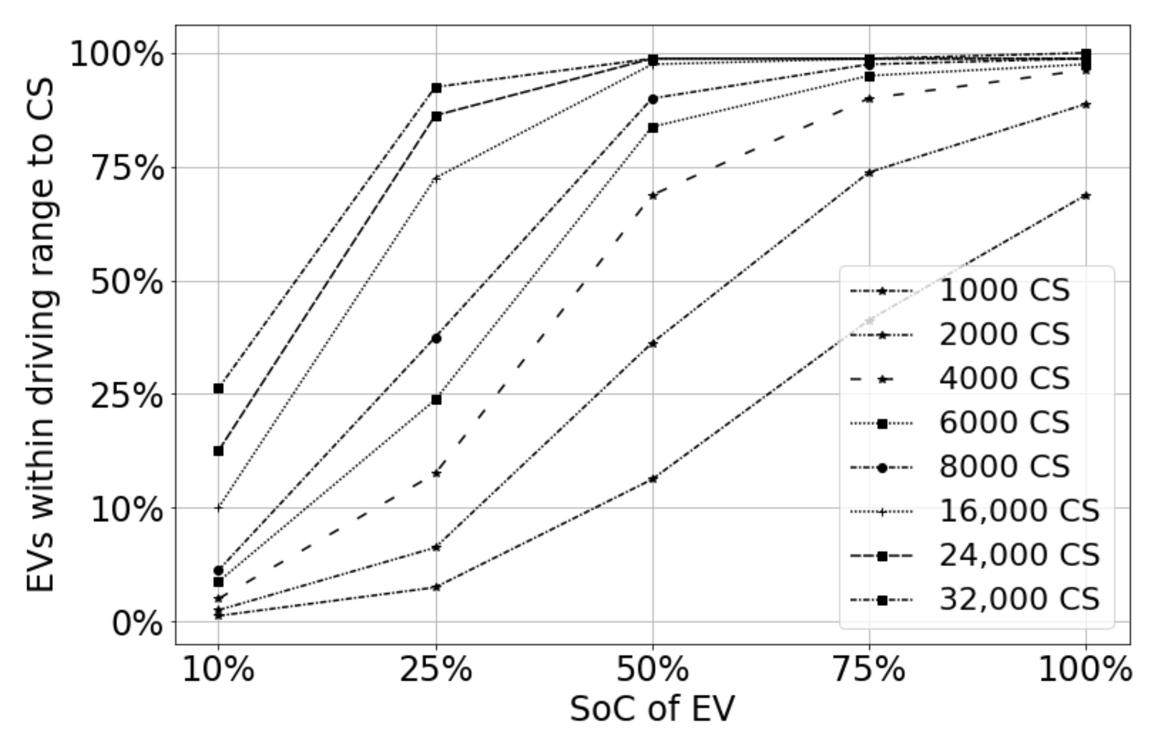
The present work is distinct in that we answer some of the practical questions of EV users and urban planners: (i) Given a city and a layout with several CSs, what is the standard recommendation of SoC for EV users to go for charging with a high success rate in finding a CS nearby? (ii) Given the EVP of an area and the quality of service, i.e., SoC, what is the CS requirement? (iii) How does the CS need planning change when the EVP changes in a planning area? In other work [24], EV charge scheduling solutions have been proposed and evaluated considering the charging rates, traffic congestion, scalability, and waiting time at a charging station.

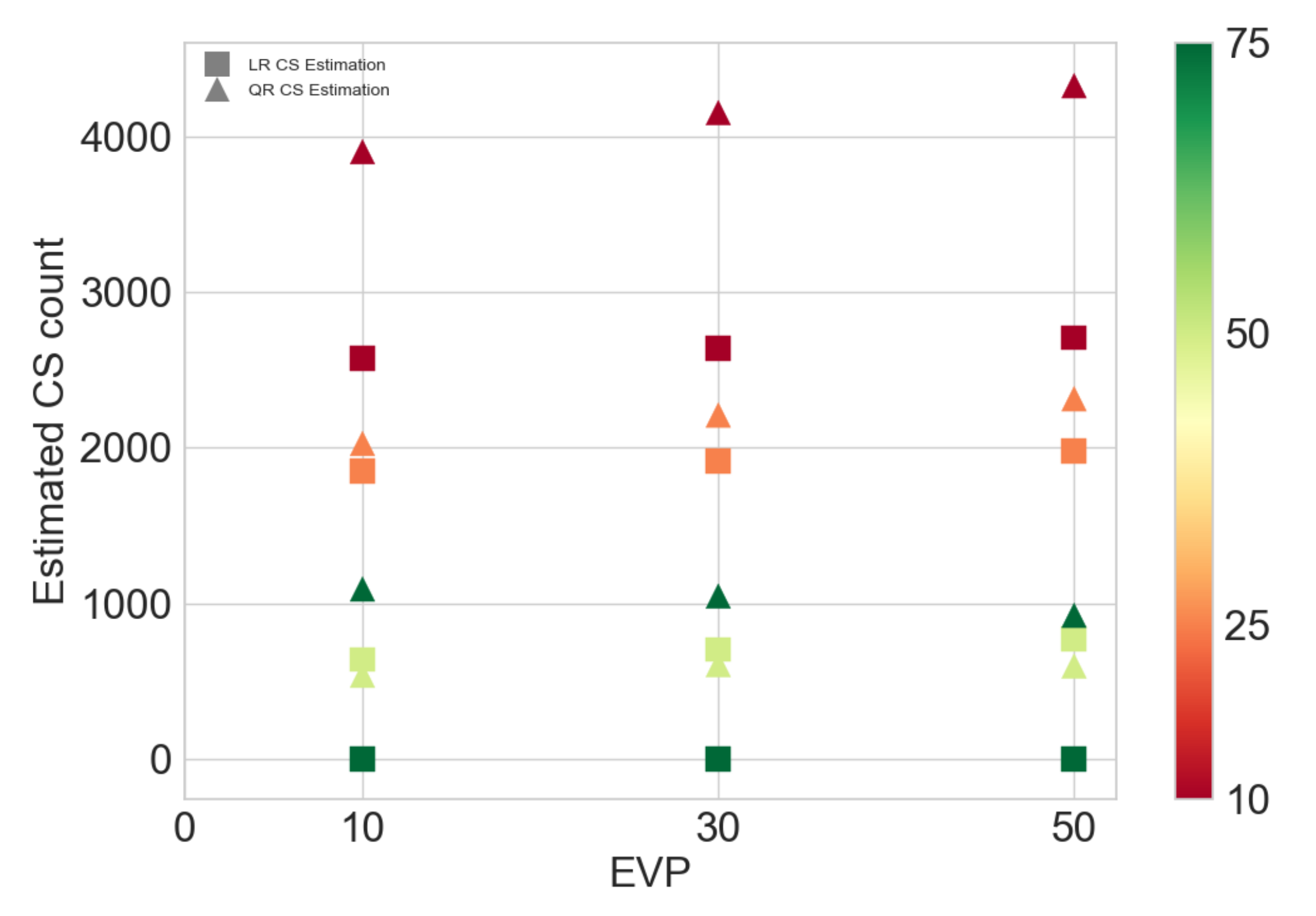
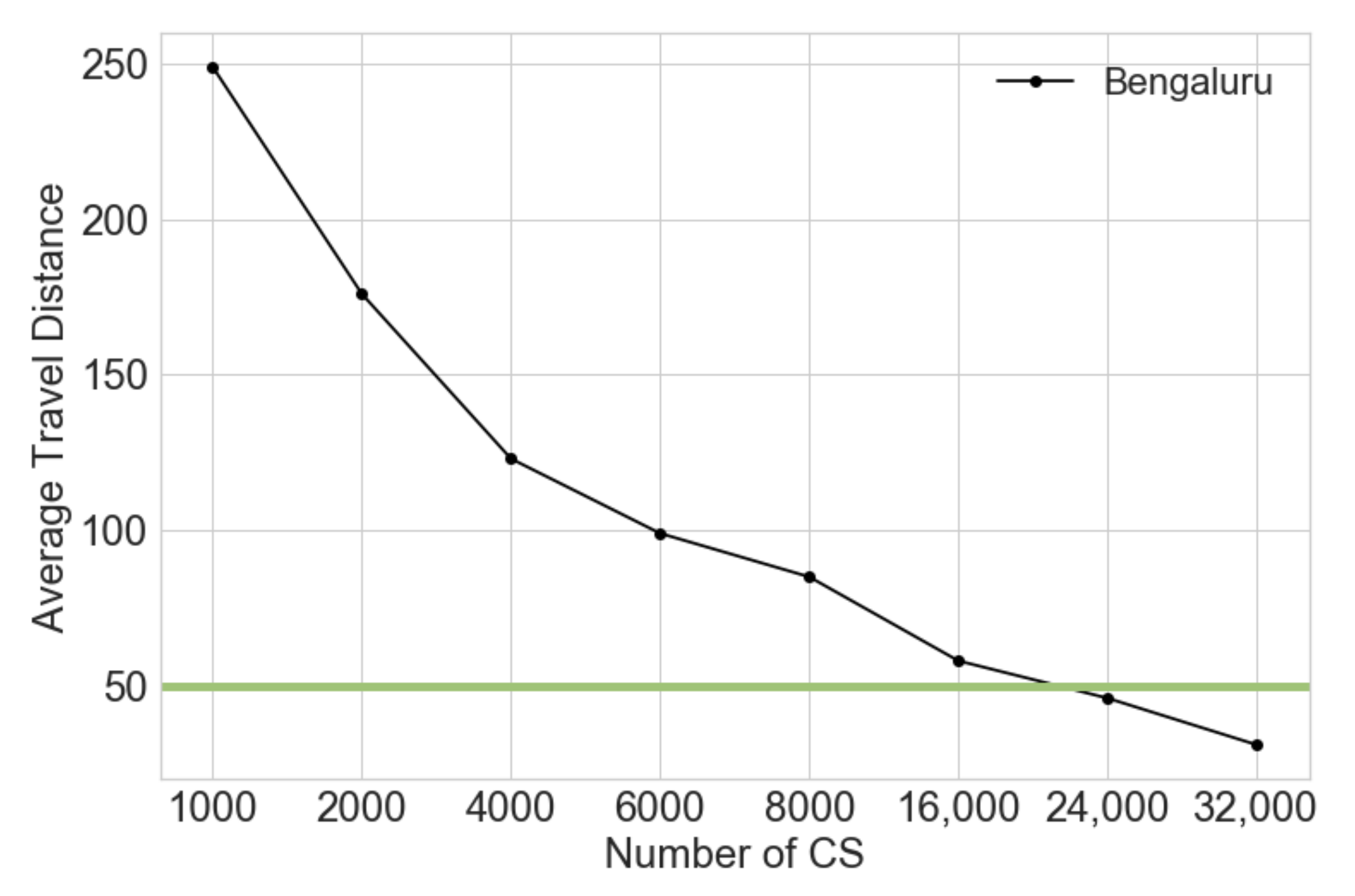
In our work, we have undertaken an impact analysis of key parameters, such as SoC, EV driving range, Average Travel Distance (ATD) of EV for a given SoC, and most importantly EVP, on the CS need estimation. We investigate some of the relationships between key CS need estimation parameters: (i) the CS size vs. EV allowable driving range relationship, (ii) the EV ATD and the number of installed CSs for different EVPs, and (iii) the CS need estimation variation with a varying EVPs for different SoCs. Another major contribution of this work is in identifying the CS size for a planning area without any adjustment factors, unlike traditional methods. Furthermore, the differences in CS estimation using (a) theoretical calculation, (b) machine learning, and (c) simulation were identified.

Overall, the key contributions of this paper are as follows:

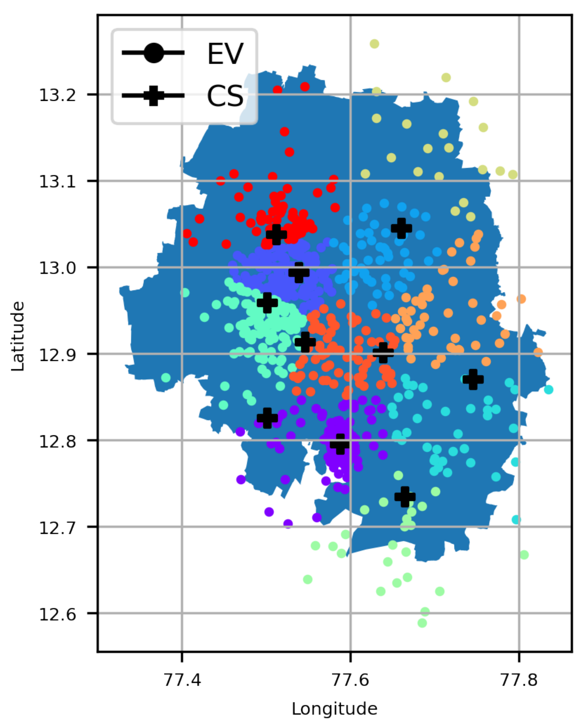
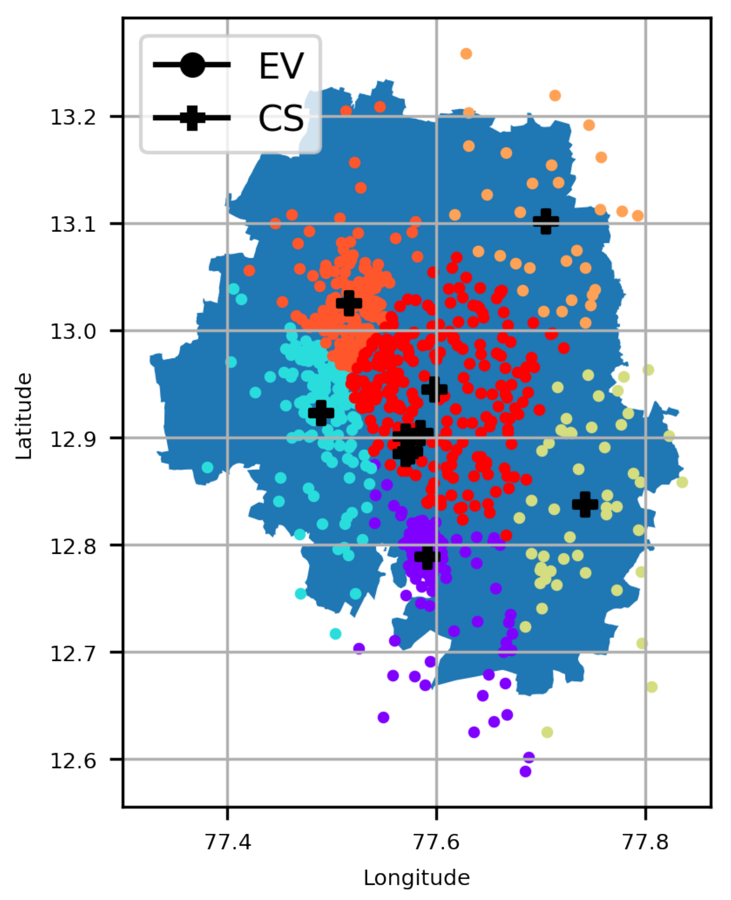
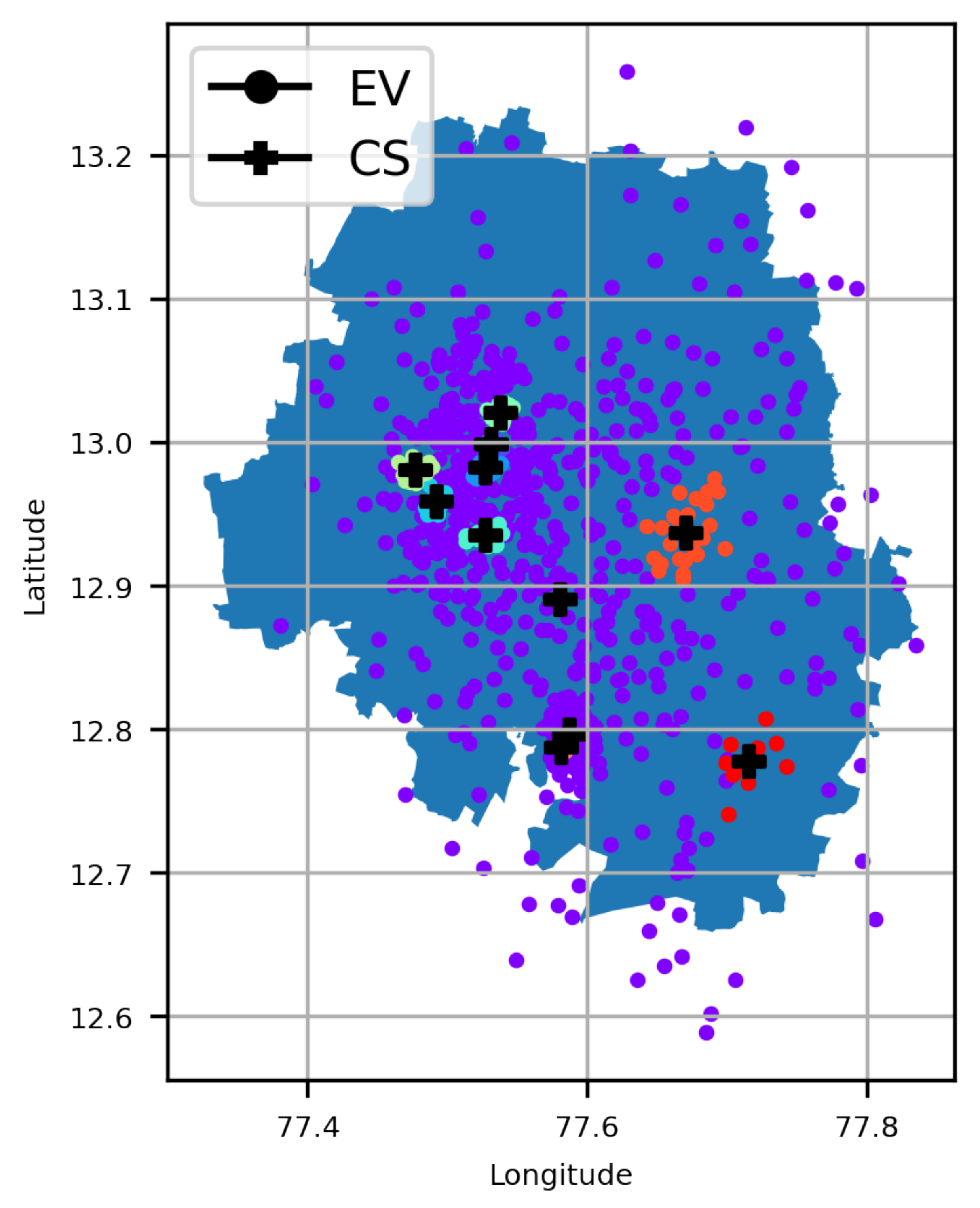
• A major contribution of this work is the investigation of optimal CS placement, i.e., EVCSP solutions using (i) different classes of clustering solutions, i.e., mean-based, density-based, spectrum- or eigenvalues-based, and Gaussian distribution; (ii) multiple metrics, i.e., (a) CS placement metrics and (b) clustering metrics, to evaluate if the clustering is good or not from a clustering perspective and an EV owners perspective, i.e., an acceptable distance to the nearest CS; and (iii) a visual understanding of the pros and cons of actual CS placements.
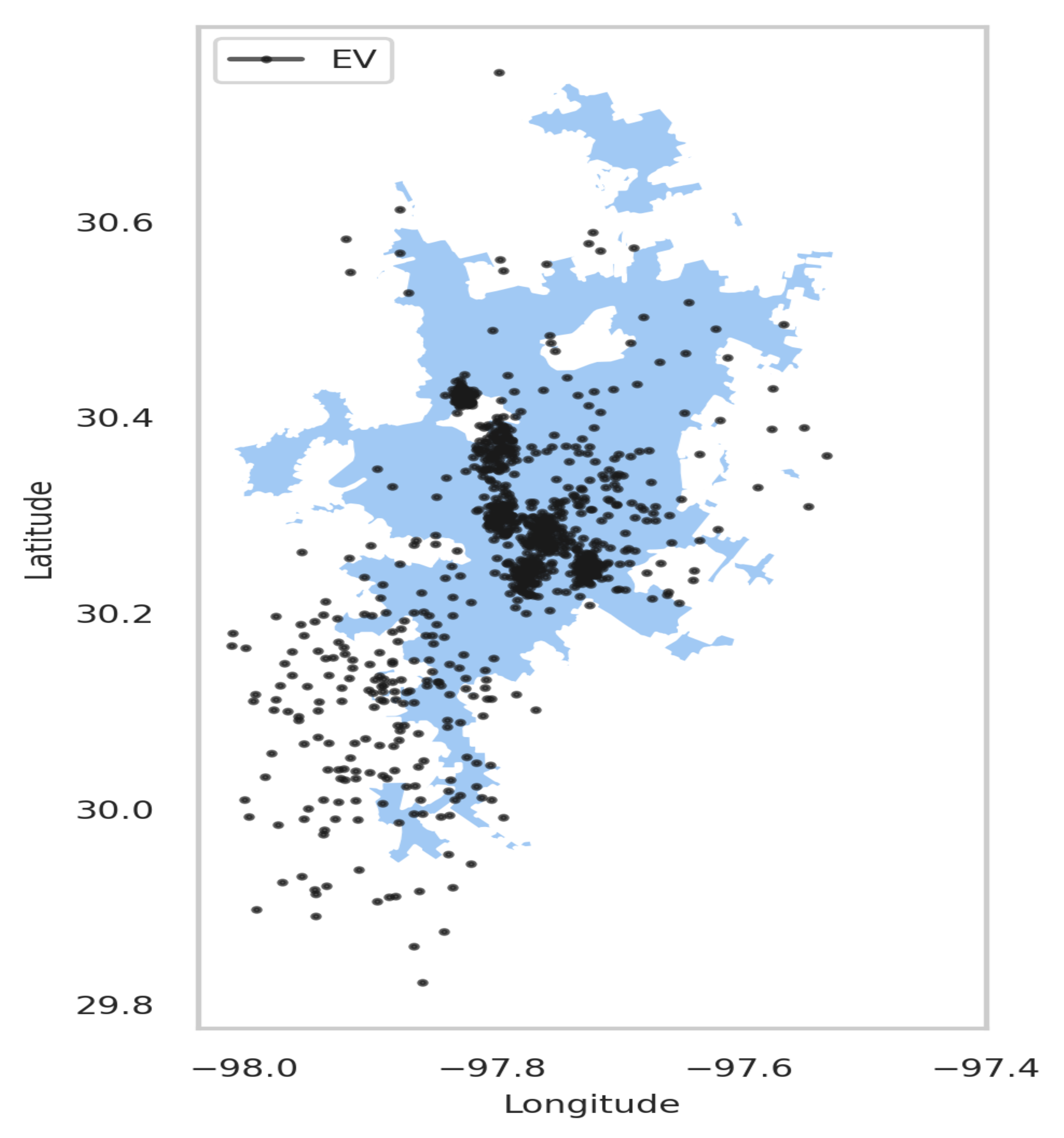
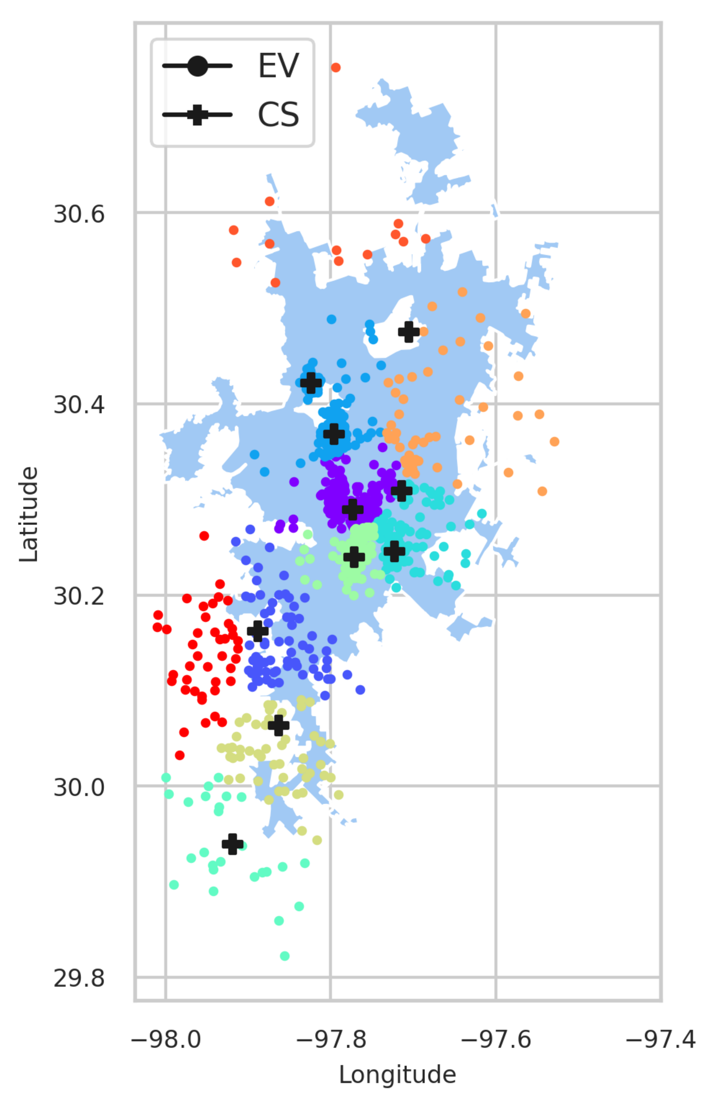
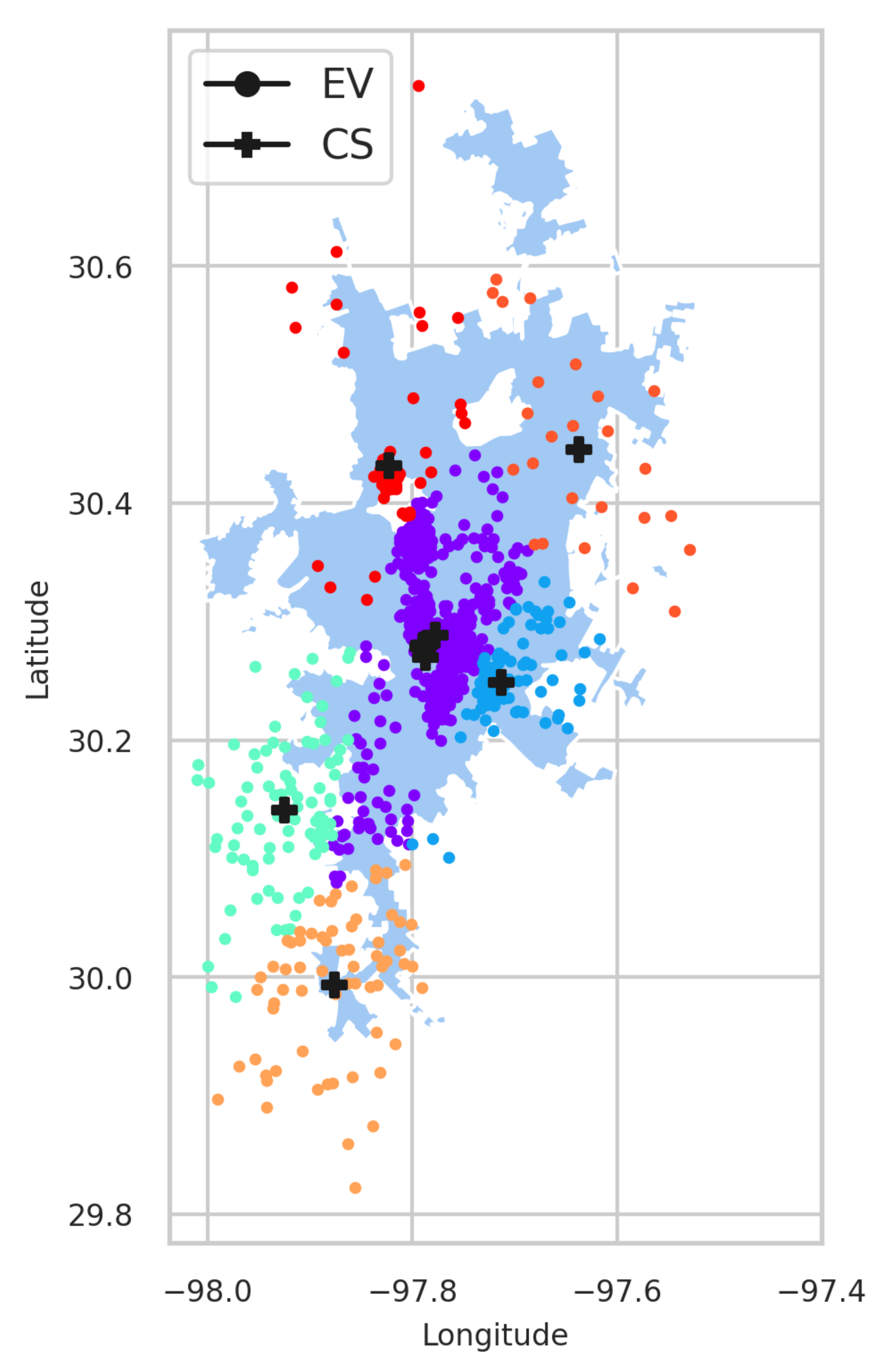
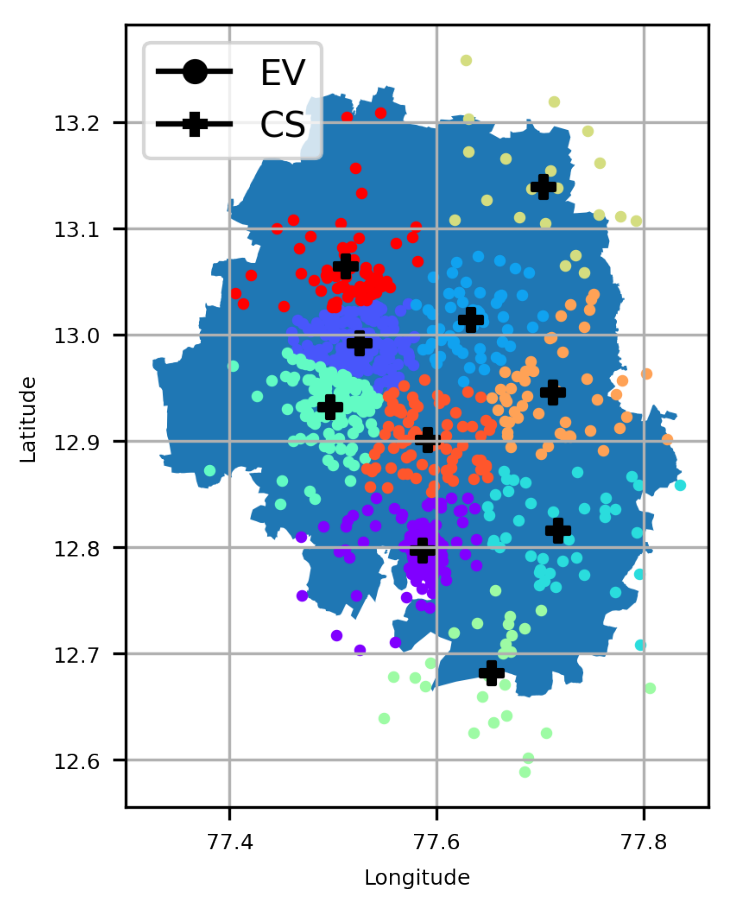
• The EVCSP solutions were evaluated in two planning areas: the Austin area with real CS data to show the improvement over the existing setup, and a greenfield area like Bengaluru, where synthetic CS data is used.
• A research gap in the CS need estimation was addressed, viz., the exclusion of SoC, EVP, and the EV driving range for CS need estimation.
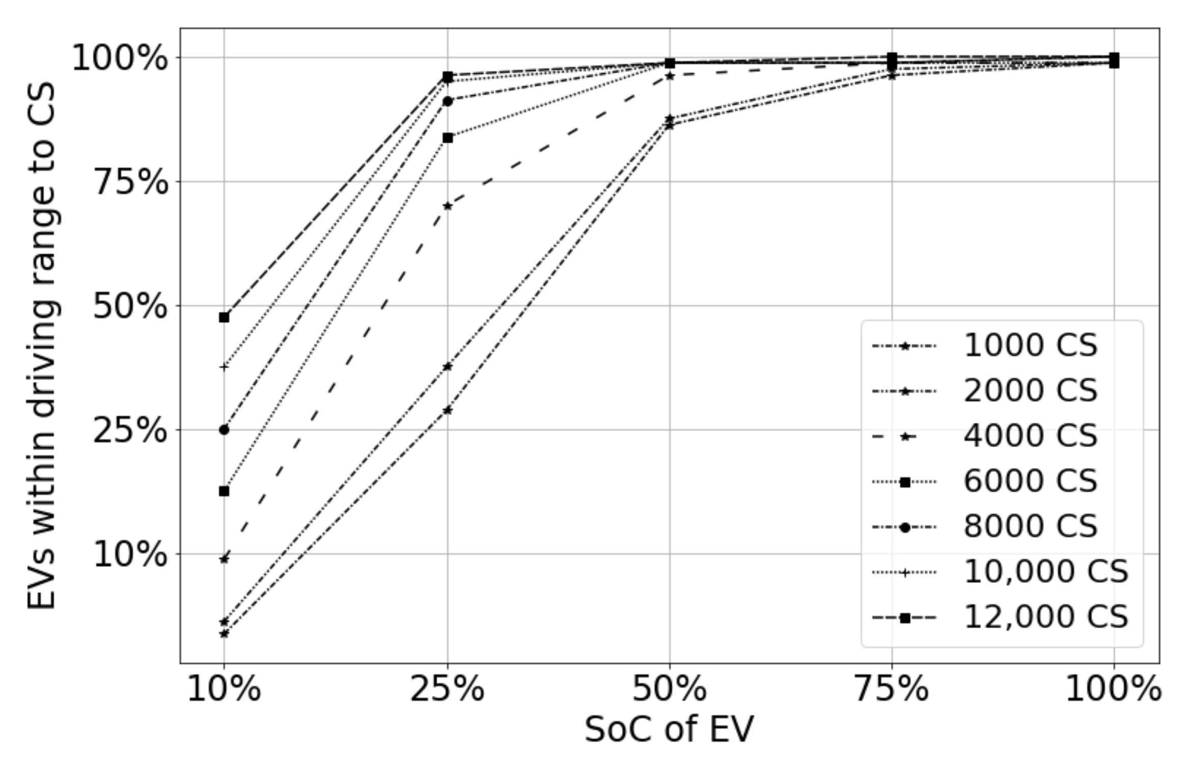
• Some of the practical questions of EV users and urban planners were answered both quantitatively and qualitatively: (i) Given a city and a layout of several CSs, what is the standard recommendation of SoC for EV users to go for charging with a high success rate in finding a CS nearby? (ii) Given the EVP of an area and the quality of service, i.e., SoC, what is the CS requirement? (iii) How does the CS need planning change when the EVP changes in a planning area?
• The relationships between CS need estimation parameters were identified: (i) the CS need estimation variation with varying EVPs for different SoCs; (ii) the EV ATD and the number of installed CSs for different EVP; and (iii) the CS size vs. the EV allowable driving range relationship and the EV driving feasibility were identified.
• Another major contribution of this work is in identifying an explainable CS need for a planning area without any adjustment factors, unlike traditional methods. Moreover, the differences in CS estimation using (a) theoretical calculation, (b) machine learning, and (c) simulation-based approach were identified. Furthermore, this work provides urban planners and EV owners with an explainable CS need estimation for the present and the future.

2. Background

Numerous EVCSP solutions have been developed by researchers. Liu et al. [25] determined CS locations using a Voronoi diagram [26] by focusing on the service radius of EVs and environmental factors. Andy et al. [27] utilized a hierarchical clustering analysis to solve EVCSP. Heuristic, numerical and analytical methods [5,28,29,30] have also been used for the CS placement of EVs, but the EVCSP is solved by assuming some fixed point equations to formulate a relationship between EV users and CSs. Clustering algorithms such as K-means [11] and agglomerative clustering [12] have been used for solving EVCSP. However, other classes of clustering methods have not been investigated in the EVCSP context.

Some later studies [31,32] have also used evolutionary algorithms for EVCSP, but they have been used when multiple objectives are involved along with EVCSP. Moreover, it has been shown [33] that clustering methods are better compared to evolutionary algorithms due to their simplicity, operational efficiency, and reduced average distance for the CS. In our work, four classes of clustering method, i.e., mean-based, density-based, spectrum- or eigenvalues-based, and Gaussian distribution were employed for EVCSP. The EVCSP clustering methods are further explained in Section 2.1.

The Mixed Integer Linear problem (MILP) [6] has also been used, but the focus is to minimize the energy consumption of EVs to reach CSs. Game theory frameworks [9] have been developed for EVCSP, but they concentrate on mileage anxiety from the EV user’s perspective only. Bae et al. [34] has developed a game approach to solve EVCSP based on EV user preference and crowdedness. A graph-based approach [7] has been developed to limit vehicle waiting times at all stations below a desirable threshold level, but a synchronization protocol is assumed for the network. The Monte Carlo simulation [23] has been used for CS placement problems, but the focus is to avoid grid expansion and avoid power losses. Many of these solutions are complex and have been tested with at most, one dataset or planning area.

Evolutionary and nature-inspired algorithm-based solutions [35,36,37,38,39,40,41] have been developed for CS placement problems, but they have advantages only when a multi-objective problem like power flow [31] or a battery weight problem [32] is explicitly defined. Dong et al. [33] have shown that clustering algorithms have performed better than evolutionary algorithms like PSO in terms of their operational efficiency and reduced average distance for the CS.

2.1. EVCSP Clustering Methods

A data point in an EVCSP corresponds to an EV x location in a planning area, and K cluster centroids correspond to N charging stations, i.e., $N_{CS}$ locations. The EVSCP clustering methods produce clusters where each cluster center represents a CS and the cluster points correspond to the EVS assigned to the same CS.

K-means [42] clustering is an unsupervised learning algorithm to solve a clustering problem. It is a hard clustering algorithm to classify a given data set into the given K clusters so that the within-cluster sum of squares is minimized. Partitioning the data set into K mutually exclusive clusters is done in such a way that data points within each cluster remain as close as possible to each other, but as far as possible from a data point in other clusters.

The spectral clustering (SC) [43] algorithm uses top eigenvectors of a matrix derived from the distance between data points. SC partitions a given data set into disjoint clusters with data points in the same cluster having high similarity and data points in different clusters having low similarity. This partitioning is then applied recursively to find K clusters.

OPTICS [44] is a hierarchical density-based data clustering algorithm that discovers arbitrary shaped clusters. It will create a reachability plot that is then used to extract clusters using an input $ϵ$. The minimum $ϵ$ denotes the core distance to make a distinct point a core point, given a finite MinPts, i.e., minimum data points to consider.

The Gaussian mixture model [45] is a probabilistic algorithm that assumes all the data points are generated from a mixture of a finite number of Gaussian distributions with unknown parameters. It is seen as a generalized K-means clustering to incorporate information about the covariance structure of the data as well as the centers of the latent Gaussians.

2.2. EVCSP Metrics

The performances of four clustering algorithms were compared in two aspects: (i) CS placement metrics and (ii) clustering metrics. The CS placement metrics comprise two parts: (i) the average distance of the EVs to the nearest CS (in km) and (ii) the maximum distance of the EVs to the nearest CS (in km). The cluster centers correspond to the CS placement location. The standard clustering metrics are defined by three scores [46,47] when the ground truth, i.e., the correct CS for an EV, is not available: (i) the Silhouette Coefficient [48] to identify incorrect clustering and overlapping clusters using intra-cluster and inter-cluster distances of EVs; (ii) the Calinski-Harabasz index [49] to identify how dense and well separated clusters are; and (iii) the Davies-Bouldin index [50] to identify the average similarity between clusters.

The Silhouette Coefficient is defined for each EV x and is composed of two scores: the average distance between an EV and all other EVs in the same cluster, i.e., $a\left(x\right)$, and the average distance between an EV and all other EVs in the next nearest cluster, i.e., $b\left(x\right)$. The Silhouette Coefficient for a set of EVs is given as the mean of the Silhouette Coefficient for each EV and is calculated [46,47] as

$$\mathbf{S}={\displaystyle \frac{1}{N_{CS}}}\sum _{i=1}^{N_{CS}}\{{\displaystyle \frac{1}{n_i}}\sum _{x\in C_i}{\displaystyle \frac{b\left(x\right)-a\left(x\right)}{max\left(b\right(x),a(x\left)\right)}}\}$$

(1)

where $C_i$ is the cluster i, $n_i$ is the number of EVs in $C_i$, $a\left(x\right)$ is the average distance between an EV x and all other EVs in the same cluster, $b\left(x\right)$ is the average distance between an EV x and all other EVs in the next nearest cluster, and $N_{CS}$ denotes the number of CSs or clusters in a planning region. The best value is 1 for a highly dense cluster and the worst value is −1 for incorrect clustering. This score is higher when clusters are dense and well separated. Negative values indicate incorrect clustering and scores near zero indicate overlapping clusters.

The Calinski-Harabasz index is also known as the Variance Ratio Criterion and is used when the ground truth is not known. It is calculated as a ratio between the within-cluster dispersion and the between-cluster dispersion where dispersion is defined as the sum of distances squared. The Calinski-Harabasz index is calculated [46,47] as

$$\mathbf{CH}={\displaystyle \frac{{\sum }_i{n}_i\times d^2(c_i,c)/N_{CS}-1}{{\sum }_i{\sum }_{x\in C_i}{d}^2(x,c_i)/N_{EV}-N_{CS}}}$$

(2)

where $d(.)$ is the distance function, c is the center of the planning area, and $N_{EV}$ denotes the total number of EVs in the planning area. The score is related to a model with better-defined clusters. It is higher when clusters are dense and well separated.

The Davies-Bouldin index denotes the average similarity between clusters, where the similarity is a measure that compares the distance between clusters with the size of the clusters themselves. The Davies-Bouldin index is computed [46,47] as

$$\mathbf{DB}={\displaystyle \frac{1}{N_{CS}}}\sum _{i=1}^{N_{CS}}\underset{j,j\ne i}{max}\{[{\displaystyle \frac{1}{n_i}}\sum _{x\in C_i}d(x,c_i)+{\displaystyle \frac{1}{n_j}}\sum _{x\in C_j}d(x,c_j)]/d(c_i,c_j)\}$$

(3)

The index relates to a model with better separation between the clusters. Zero is the lowest possible score and values closer to zero indicate a better clustering.

2.3. CS Need Estimation: Traditional Approach

The number of EVs in a planning region will depend on the number of households, EVP, and the number of vehicles per household. The electricity demand of an EV per day will depend on P, the power consumption of the EV, and the distance traveled by the EV per day [14]. The average electricity demand of an EV per day is denoted by $P_{avg}$. $P_{avg}$ is calculated as below:

$$P_{avg}=P\times r\times cycles$$

(4)

where $P_{avg}$ is the power consumption of the EV in kWh/mile, r is the battery range of the EV in miles, $cycles$ denotes the charge cycles per day.

The total electricity demand denoted by W in an area is calculated below:

$$W=P_{avg}\times N_{EV}$$

(5)

where $N_{EV}$ is the number of EVs in a planning region

The number of charging stations $N_{CS}$ required in a planning region is calculated as below:

$$N_{CS}=\beta \times \frac{W}{P_{CS}\times T_{EV}}$$

(6)

where $\beta$ is an adjustment constant factor used in prior works [14,15] for the theoretical estimation of CS need, $P_{CS}$ is the capacity of CS, and $T_{EV}$ is the time needed to charge an EV to its full capacity.

3. EV Charging Station Planning

3.1. EVCSP Problem Formulation

The EVCSP problem is defined for a planning region using a directed graph or transportation network $\mathbf{G}(\mathbf{V},\mathbf{E})$, where $\mathbf{V}=\{v_0,v_1,\dots ,v_n\}\mathrm{and}\mathbf{E}=\left\{(v_i,v_j)\right|(v_i,v_j)\in V^2;i\ne j\}$ represent a set of vertices and a set of edges, respectively.

$\mathbf{V}$ represents intersections, or designated points on roads, and $\mathbf{E}$ represents all roads in the transportation network $\mathbf{G}(\mathbf{V},\mathbf{E})$. We assume all CSs are located on some subset of $\mathbf{V}$ [51].

The common terms used in EVCSP are range, route, Electric Vehicle (EV), CS, planning region, EV penetration (EVP), state of charge (SoC), and Average Travel Distance (ATD). The range of an EV represents the distance the EV can travel without recharging [52]. The shortest path between any given origin and destination vertices for an EV is the route. The planning region is a geographical area of interest for the CS placement study. EVP represents the percentage of EV vehicles used by people in a planning region. The ATD represents the average of the distances an EV can travel given a current SoC.

We use $c_i$ to denote a particular CS with index i, but use c when only one CS is being referred to. We use $x_j$ to denote an EV indexed by j, but use x when only one EV is being referred to. The current range of an EV indicates how far the EV can travel without recharging [53]. The criteria for the driving range limit of an EV is the state of charge (SoC) that depends on its current range.

In a planning region, the basic aim of EVCSP is to identify a CS for each EV such that the total distance traveled by the EV owners for charging at the nearest CS is minimized; this is calculated by the objective function as defined in (1).

$$\min F=\sum _i^{N_{CS}}\sum _j^{N_{EV}}{\lambda }_{i,j}{∥c_i-x_j∥}_2$$

(7)

where $N_{EV}$ denotes the number of EVs and $N_{CS}$ denotes the number of CSs in a planning region.

The ${\lambda }_{i,j}$ used in (1) is calculated as

$${\lambda }_{i,j}=\left\{\begin{array}{c}1,\mathrm{if}{c}_i\mathrm{is}\mathrm{the}\mathrm{nearest}\mathrm{CS}\mathrm{to}\mathrm{EV}{x}_j\hfill \\ 0,\mathrm{if}{c}_i\mathrm{is}\mathrm{not}\mathrm{the}\mathrm{nearest}\mathrm{CS}\mathrm{to}\mathrm{EV}{x}_j\hfill \end{array}\right.$$

(8)

3.2. Datasets and Experimental Setup

3.2.1. Planning Areas

Two planning areas with EV households, i.e., houses with an EV, are shown in Figure 1 and Figure 2 were used for the following experiments. The units of the plots in Figure 1 and Figure 2 are degrees. The longitude is on the x-axis and latitude is on the y-axis in our 2D plots, which are projections onto a plane. The first area has real CS data [54] and represents Austin, Texas, in the United States. Bengaluru is a major transportation hub. The second area is a synthetic one, representing Bengaluru, Karnataka, India.

3.2.2. Experimental Setup

In this study, the EV households were set to 10,000 for the Austin and Bengaluru areas, referring to the Austin EV count in 2020 [55] for the comparative performance of all algorithms. The real CS count of 467 [54] for the Austin area and a CS count of 1000 for the Bengaluru area were fixed for the performance comparison in Section 4.1.

EVPs of $10\%,30\%,\mathrm{and}50\%$ and SoCs of $10\%,25\%,50\%,75\%,\mathrm{and}100\%$ were considered in Section 4.2 for the impact analysis of EVP and SoC on the CS need estimation. To simulate large-scale EVCSP experiments, i.e., to understand scalability, the CS count was increased to large numbers, i.e., 2000, 4000, 6000, 8000, 10,000, and 12,000 for Austin and 2000, 4000, 6000, 8000, 16,000, 24,000, and 32,000 for Bengaluru. The EV count was set to 190,000 and 650,000 for Austin and Bengaluru, respectively based on their population [55,56] and by referring to an EVP of $50\%$ for the impact analysis in Section 4.3.

Different types of zones were simulated with varying densities of EVs in both the planning areas. The density of EVs in the Bengaluru area was set to twice the density of EVs in Austin.

Two different types of AWS instances, i.e., r5.8x.large of 258 GB RAM, and r5.4x.large of 128 GB, were used for the experiments due to the high RAM and computation requirements.

This paper studies the EVCSP problem from the global optimization perspective of an EV-hailing company and adopts the EV driving range limit criteria as seen elsewhere [51]. The driving range limit of currently available EVs is in the range of 150–550 km [57]. A average driving range limit of 312 km was considered for the EVs referring to the Tata Motors Nexon Model [58].

3.3. Assumptions

The underlying assumptions of our work are that EV drivers go to a charging station when the SoC is low [59,60] (rather than using only home and office chargers) and heavily use charging stations near to their homes [61].

The charging behavior is similar to Hu et al. [59] and Yang et al. [60] where EV drivers have charging station choices and may ask a navigation service for advice on which charging station to use [61]. Moreover, EV drivers would go to a charging station only if the battery, i.e., SoC, is low or drops below a certain level.

In earlier works [3,14,26,62], the CS placement focused on the coverage or service radius extension across a city, and the location of households was used for the CS placements. Our work is also in line with these, and another key objective of the CS placement when considering households is the EV owners’ convenience, i.e., a preference for overnight charging near their homes due to high charging times. It is worth noting that while gas stations can be placed at intermediate locations on roads and highways, this is largely because filling up with fuel is a quick matter, taking minutes in most cases, unlike EV charging which is far slower.

4. Results

4.1. Comparative Performance of All Algorithms

This section compares the performances of four clustering algorithms in two aspects: (i) CS placement metrics and (ii) clustering metrics. The CS placement metrics comprise two parts: (i) the average distance of the EVs to the nearest CS (in km) and (ii) the maximum distance of the EVs to the nearest CS (in km). The cluster centers correspond to the CS placement location. The clustering metrics [47] are defined by three scores: (i) the Silhouette Coefficient, (ii) the Calinski-Harabasz index, and (iii) the Davies-Bouldin index.

The Silhouette Coefficient is calculated using the mean intra-cluster distance and the mean nearest-cluster distance for each EV. The best value is 1 and the worst value is −1. Negative values indicate incorrect clustering and scores near zero indicate overlapping clusters. The Calinski-Harabasz index is calculated as a ratio between the within-cluster dispersion and the between-cluster dispersion where dispersion is defined as the sum of distances squared. The score is higher when clusters are dense and well separated. The Davies-Bouldin index denotes the average similarity between clusters, where the similarity is a measure that compares the distance between clusters with the size of the clusters themselves. Zero is the lowest possible score and values closer to zero indicate a better clustering.

4.1.1. Austin

The CS placement in the Austin area was evaluated using well-known clustering algorithms like K-Means, GMM, OPTICS, and SC. The CS placement was evaluated by the CS placement and clustering metrics defined in Section 4.1. Figure 3, Figure 4, Figure 5 and Figure 6 show a sample of ten CS placement locations, marked as ‘+’, along with EVs, allocated to a particular CS. The EVs allocated to the same CS are marked with the same color. The figures show that K-Means and GMM are better CS placement algorithms, while OPTICS and SC are the worst performing for the given planning area. As shown in Figure 5, the OPTICS algorithm focused on the density of the EVs to place more CSs in those locations with more EVs. So, the EVs in a less dense area need to travel to a higher density area for the nearest CS. This can be attributed to the fact that OPTICS is a density-based clustering algorithm. As shown in Figure 6, the SC algorithm placed more CSs in connected but less dense areas which are far away areas from Austin city. Moreover, the SC algorithm places a single CS in a high-density area around Austin where there is more connectivity. This can be attributed to the fact that the SC focuses on the connectivity of the points rather than compactness, which is the distance of the EVs from the nearest CS.

The metrics shown in

Table 1. CS Placement Metrics (Austin).

Metric	Existing CS Setup	SC	OPTICS	GMM	K-Means
Average distance of the EV households to the nearest CS (in km)	4.75	4.69	4.54	0.54	0.52
Maximum distance of the EV households to the nearest CS (in km)	15.62	13.55	44.06	2.14	1.38

indicate that the average distance of the EV households to the nearest CS is nine times better with K-Means and GMM over SC and OPTICS. Furthermore, the maximum distance of the EV households to the nearest CS is significantly lower with K-Means followed by GMM.

The metrics shown in

Table 2. Clustering Metrics (Austin).

Metric	Silhouette Score	Calinski-Harabasz Score	Davies-Bouldin Score
SC	−0.01	122.97	0.97
OPTICS	0.19	11.56	1.47
GMM	0.20	11,021.12	0.86
K-Means	0.24	12,614.88	0.81

indicate that K-Means and GMM are better clustering algorithms for the planning area. The existing setup column computes the scores when the real 467 CS placements in Austin are used. In the case of SC, the Silhouette score is negative indicating that the clustering is incorrect. Among K-Means and GMM, K-Means is observed to be better considering all the metrics.

4.1.2. Bengaluru

The CS placement in the Bengaluru area was evaluated using well-known clustering algorithms like K-Means, GMM, OPTICS, and SC. The CS placement was evaluated by the CS placement and clustering metrics defined in Section 4.1.

Figure 7, Figure 8, Figure 9 and Figure 10 show a sample of ten CS placement locations, marked as ‘+’, along with EVs, allocated to a particular CS. The figures show that K-Means and GMM are better CS placement algorithms while OPTICS and SC are the worst performing for the given planning area. As shown in Figure 9, the OPTICS algorithm focused on the density of the EVs to place more CSs in those locations with more EVs. The OPTICS algorithm CS placement performance improved compared to the Austin area, i.e., there are some CS placements in a less dense area and more CS placements in a higher density area. This can be attributed to the fact that the Bengaluru area has twice the density of the Austin area and OPTICS is a density-based clustering algorithm. As shown in Figure 10, the SC algorithm placed more CSs in connected but less dense areas which are far away from Bengaluru city. Moreover, the SC algorithm places a single CS in a high-density area around Bengaluru where there is more connectivity. This can be attributed to the fact that the SC focuses on the connectivity of the points rather than compactness, which is the distance of the EVs from the nearest CS.

The metrics shown in

Table 3. Clustering Metrics (Bengaluru).

Metric	Silhouette Score	Calinski-Harabasz Score	Davies-Bouldin Score
SC	−0.06	57.65	1.04
OPTICS	0.19	11.91	1.45
GMM	0.22	11,626.92	0.82
K-Means	0.25	13,619.86	0.78

indicate that K-Means and GMM are better clustering algorithms for the planning area. In the case of SC, the Silhouette score is negative indicating that the clustering is incorrect. Among K-Means and GMM, K-Means is observed to be slightly better considering all the metrics.

The metrics shown in

Table 4. CS Placement Metrics (Bengaluru).

Metric	SC	OPTICS	GMM	K-Means
Average distance of the households to the nearest CS (in km)	4.42	4.83	0.35	0.33
Maximum distance of the households to the nearest CS (in km)	14.45	43.00	1.85	0.92

indicate that the average distance of the EV households to the nearest CS is 15 times better with K-Means and GMM over SC and OPTICS. Moreover, the maximum distance of the EV households to the nearest CS is significantly lower with K-Means followed by GMM.

4.2. Impact Analysis: CS Need Estimation Using SoC and EVP

An EV’s travel distance to the nearest CS depends significantly on constant factors like the vehicle class and variable factors like SoC and traffic flow due to the EVP in a planning area [15]. The impact analysis was undertaken on both the planning areas with different EVPs, i.e., 10%, 30%, and 50%, and with different SoCs, i.e., 10%, 25%, 50%, and 75%. The methods described in this section use the simulation data obtained from the different configurations above to build two machine learning models for CS need estimation, i.e., linear regression and quadratic regression of degree two. As presented in Figure 11 and Figure 12, the horizontal dimension represents EVP, and the vertical dimension represents the estimated CS count. The square box represents the linear regression estimates and the triangular box represents the quadratic regression estimates. The color of the box represents different SoCs as shown in the color bar.

In Figure 11, we see that the CS count estimation using LR is the worst as the estimation is showing only a slight increase or the same CS count for an increasing EVP and for SoCs of 10% and 25%. In contrast, the QR CS estimation is increasing with increasing EVP and for SoCs of 10% and 25%. Moreover, we see that LR has given a near-zero estimation for the CS count when the SoC is 75% whereas the QR estimation is near to 1000 CS. The LR and QR estimations for a SoC of 50% are similar.

The performance of the QR algorithm is better due to a better RMSE over LR and due to the contribution of nonlinear prediction components. This is shown in

Table 5. CS Need Estimation Models for Austin.

Method	RMSE	Intercept	${\mathit{\alpha }}_{\mathit{evp}}$	${\mathit{\alpha }}_{\mathit{soc}}$	${\mathit{\alpha }}_{\mathit{evp}}^2$	${\mathit{\alpha }}_{\mathit{soc}}^2$	${\mathit{\alpha }}_{\mathit{evp}}\times {\mathit{\alpha }}_{\mathit{soc}}$
Linear Regression	151.41	3024.82	3.29	−48.34	-	-	-
Quadratic Regression (deg = 2)	19.07	5379.71	18.73	−179.76	−0.09	1.63	−0.23

. Moreover, this study establishes the significant advantages of using nonlinear CS estimation models.

In Figure 12, we see that the CS count estimation using LR is better than in the Austin case, but it is still the worst as the estimation is showing only a slight increase or the same CS count for an increasing EVP and for all SoCs. In contrast, the QR CS estimation is increasing with increasing EVP and for all SoCs.

The performance of the QR algorithm is better due to a better RMSE over LR and due to the contribution of nonlinear prediction components. This is shown in

Table 6. CS Need Estimation Models for Bengaluru.

Method	RMSE	Intercept	${\mathit{\alpha }}_{\mathit{evp}}$	${\mathit{\alpha }}_{\mathit{soc}}$	${\mathit{\alpha }}_{\mathit{evp}}^2$	${\mathit{\alpha }}_{\mathit{soc}}^2$	${\mathit{\alpha }}_{\mathit{evp}}\times {\mathit{\alpha }}_{\mathit{soc}}$
Linear Regression	797.83	6221.80	13.46	−69.38	-	-	-
Quadratic Regression (deg = 2)	121.02	8796.79	18.55	−174.74	−0.02	0.93	−0.20

. One interesting finding is that the expected mean CS estimation, i.e., the intercept, is 3024 for Austin and 6221 for Bengaluru using LR estimation and it is 5379 and 8796 using QR estimation, which is a 3000 CS difference in estimation.

4.3. Impact Analysis: CS Need Estimation Using SoC, EV Driving Range, and ATD

A CS need estimation for the future depends on SoC, the average EV driving range, and the ATD of an EV to reach the nearest CS. An impact analysis was undertaken of increasing CSs on the ATD and the feasibility of EVs to reach the nearest CS with a given SoC. The methods described in this section are based on the simulations which internally used the best CS placement algorithms, i.e., K-Means, and GMM. The impact analysis was performed on both the planning areas with the best CS placement algorithms and with different average SoCs of EVs before going for charging, i.e., 10%, 25%, 50%, 75%, and 100%, and for an EVP of 50%. Moreover, the inclusion of key parameters such as SoC, EV Driving Range, EV penetration (EVP), and Average Travel Distance (ATD) was a revised practical approach for CS need estimation unlike the traditional method described in Section 2.3 and Section 5.1. A large CS count of up to 12,000 and 32,000 were evaluated for the Austin and Bengaluru areas, respectively. As presented in

Table 7. Estimated Austin CS count using the ATD of K-Means for a 50% EVP.

SoC of an EV	Feasible EV Range to Reach the Nearest CS (km)	K-Means
		1000	2000	4000	6000	8000	10,000	12,000
10%	32	126	87	60	47	40	35	31
25%	78	126	87	60	47	40	35	31
50%	156	126	87	60	47	40	35	31
75%	234	126	87	60	47	40	35	31
100%	312	126	87	60	47	40	35	31

,

Table 8. Estimated Austin CS count using the ATD of GMM for a 50% EVP.

SoC of an EV	Feasible EV Range to Reach the Nearest CS (km)	GMM
		1000	2000	4000	6000	8000	10,000	12,000
10%	32	126	88	61	50	43	38	32
25%	78	126	88	61	50	43	38	32
50%	156	126	88	61	50	43	38	32
75%	234	126	88	61	50	43	38	32
100%	312	126	88	61	50	43	38	32

,

Table 9. Estimated Bengaluru CS count using the ATD of K-Means for an EVP a 50%.

SoC of an EV	Feasible EV Range to Reach the Nearest CS (km)	K-Means
		1000	2000	4000	6000	8000	16,000	24,000	32,000
10%	32	249	176	123	99	85	58	46	31
25%	78	249	176	123	99	85	58	46	31
50%	156	249	176	123	99	85	58	46	31
75%	234	249	176	123	99	85	58	46	31
100%	312	249	176	123	99	85	58	46	31

and

Table 10. Estimated Bengaluru CS count using the ATD of GMM for an EVP of 50%.

SoC of an EV	Feasible EV Range to Reach the Nearest CS (km)	GMM
		1000	2000	4000	6000	8000	16,000	24,000	32,000
10%	32	251	178	124	100	87	61	48	32
25%	78	251	178	124	100	87	61	48	32
50%	156	251	178	124	100	87	61	48	32
75%	234	251	178	124	100	87	61	48	32
100%	312	251	178	124	100	87	61	48	32

, the numbers 1000 to 32,000 in the horizontal dimension represent cases when different numbers of CSs are deployed using either the K-Means or GMM method in the Austin or Bengaluru area. The first column in the tables represents different SoC cases, i.e., at what SoC of the EV battery does the EV driver decide to go for charging. The second column lists the feasible range of the EV with the SoC given in the first column. The values in the other column represent the ATD of the EVs with the given SoC when the number of CSs deployed in the Austin or Bengaluru area is known. The CS count for an average SoC in a planning area is feasible, marked as green cells, if the ATD of the EVs with the given SoC is within the range to reach the nearest CS. The case of a marginally feasible CS count, marked as yellow cells, is when the ATD of the EVs is closer to, but not within, the average EV range to reach the nearest CS. The infeasible CS count is marked with red cells when the ATD is very high.

The estimated CS count for Austin is shown with respect to feasibility. As shown, 6000 to 10,000 CSs is a marginally feasible count as per K-Means and GMM, though the ATD with GMM CS placement is slightly higher than with K-Means as shown in Table 7 and Table 8. However, 12,000, 4000, 2000, 1000, and 1000 CSs are a minimum feasible CS count for a SoC of 10%, 25%, 50%, 75%, and 100%, respectively for the Austin area with both the CS placement algorithms. It is interesting to note that the estimated CS count doubles from 2000 to 4000 when the SoC is decreased from 50% to 25%, and triples from 4000 to 12,000 when the SoC is decreased from 25% to 10%, due to the nonlinear increase in the CS count requirements.

Figure 13 presents the ATD curve for an increasing CS count. The ATD curve slope sharply decreases with increasing CSs from 1000 to 6000 CSs. The CS count estimation is performed here using the ATD of the EV. The average traveling distance was found to be 51 km when fast charging was used as per recent studies [63,64]. Based on this, we take the average traveling distance to be 40–50 km as a sample cutoff, shown as a horizontal cutoff line in Figure 13 and Figure 14, for the CS need estimation. As shown in Figure 13, 6000–8000 CSs seems a reasonable CS count estimate when an ATD of 40–50 KM is considered to be feasible for an EV to travel for charging.

An analysis of the SoC of EVs and the percentage of EVs within driving range of a CS, as shown in Figure 15, finds a SoC of 25% as a recommendation for 6000–12,000 CSs in the Austin area, as it ensures more than 75% of the EVs are within driving range of a CS. On the other hand, a SoC of 50% ensures more than 75% of the EVs are within driving range, even with 1000–2000 CSs.

The estimated CS count for Bengaluru is shown with respect to feasibility. As shown, 16,000 to 24,000 CSs is a marginally feasible count as per K-Means and GMM, although the ATD with GMM CS placement is slightly higher than with K-Means as shown in Table 9 and Table 10. However, 32,000, 16,000, 4000, 2000, and 1000 CSs are a minimum feasible CS count for a SoC of 10%, 25%, 50%, 75%, and 100%, respectively for the Bengaluru area with both the CS placement algorithms. It is interesting to note that the estimated CS count increases by four times from 4000 to 16,000 when the SoC is decreased from 50% to 25%, and doubles from 16000 to 32,000 when the SoC is decreased from 25% to 10%, due to the nonlinear increase in the CS count requirements.

Figure 14 presents the ATD curve for increasing CS counts. The ATD curve slope sharply decreases with increasing CSs from 1000 to 16,000. The CS count estimation is performed here using the ATD of the EV. As shown in Figure 14, 16,000–32,000 CSs seems a reasonable CS count estimate when an ATD of 40–50 KM is considered to be feasible for an EV to travel for charging.

An analysis of the SoC of an EV and the percentage of EVs within driving range of a CS, as shown in Figure 16, finds a SoC of 25% as a recommendation for 24,000–32,000 CSs in the Bengaluru area, as it ensures more than 75% of the EVs are within the driving range of a CS. On the other hand, a SoC of 50% ensures more than 75% of the EVs are within driving range, even with 6000–8000 CSs.

5. Discussion

5.1. Traditional Approach

In the traditional approach, an EVP of 50% is considered to estimate the CS count. The values of P = 0.16 KWh/mile, r = 193 mile (312 km), and $n_c$ = 0.3 are considered referring to the Tata Nexon model [58]. The electricity demand of an EV per day, $P_{avg}$, is the same for both the planning areas and it is estimated as below using (1):

$$P_{avg}=0.16\times 193\times 0.3=9.264\mathrm{KWh}$$

Since an EVP of 50% is considered, the $N_{EV}$ is considered as 190,196 and 646,126 for the Austin and Bengaluru areas, respectively. The total electricity demand of Austin and Bengaluru is denoted by $W_A$ and $W_B$, respectively and is estimated as below using (5):

$$W_A=9.264\times 190,196=1,761,975\mathrm{KWh}$$

$$W_B=9.264\times 646,126=5,985,711\mathrm{KWh}$$

The adjustment factor $\beta$ value is 1.4 [14] and the average time needed to charge an EV to its full capacity denoted by $T_{EV}$ is taken as 1 h. The number of charging stations $N_{CS}$ estimated for Austin and Bengaluru is denoted by $N_{CS}\left(A\right)$ and $N_{CS}\left(B\right)$ is estimated as below:

$$N_{CS}\left(A\right)=1.4\times \frac{W_A}{600\mathrm{KWh}\times 1}=\frac{4,473,410}{600}=4111\approx 4100$$

$$N_{CS}\left(B\right)=1.4\times \frac{W_B}{600\mathrm{KWh}\times 1}=\frac{5,985,711}{600}=13,996\approx 14,000$$

5.2. Data Driven Approach

The CS need estimation is performed for the Austin and Bengaluru areas. As shown in

Table 11. CS Need Estimation: Summary.

Approach	Austin	Bengaluru
Traditional	4100	14,000
ML (Quadratic Regression) and SoC of 10%	4300	8000
Simulation and SoC of 10% based marginal cutoff	6000	16,000
Simulation and ATD (40–50 km) based firm cutoff	6000	24,000
Simulation and SoC of 10% based firm cutoff	12,000	32,000

, the traditional approach estimate is seen to be less as it does not consider the SoC of the EVs in the areas. Since a SoC of 10% is a more likely to cause owners of EVs to look for the nearest CS, this case is used by different approaches for the CS estimate comparison with the traditional approach. The ML approach estimation is the closest to the traditional approach estimate, but the CS estimation for the high density of the Bengaluru area is underestimated. The simulation-based approach with a marginal cutoff shows an estimate of 6000 CSs for Austin and 16,000 CSs for Bengaluru such that 75% of the EVs with a SoC of 10% have the nearest CS within their driving range. A similar approach that is based on the ATD shows an increased CS estimate for the high-density Bengaluru area. The upper bound of the CS estimation is 12,000 CSs for Austin and 32,000 CSs for the Bengaluru area. This is given by the simulation with a firm cutoff where 100% of the EVs with a SoC of 10% have the nearest CS within their driving range.

Overall, the results can be used to guide decision makers in making better CS placement decisions and CS need estimations, unlike traditional methods which are based on density for CS placement and mathematical calculations with black box adjustment factors for CS need estimations. The different models for the CS need estimation consider different factors and provide lower and upper bound estimates of the CS need. Instead of a single model-based estimate, explainable bounds for CS needs are provided for use by decision makers. It is worth mentioning that the CS need estimations can now be undertaken by different approaches to arrive at explainable lower and upper bound CS need estimates considering different factors.

6. Conclusions

Our results can be used to guide urban planners in making better CS placement approval decisions when many CSs (in the order of hundreds or more) need to be placed for charging at different locations of a planning area in an efficient manner, i.e., considering the clustering efficiency, the EV owners convenience, and the visual analysis of the system.

Using our CS need estimation methods, urban planners can estimate the CS need range, i.e., minimalist need, actual need, and future need, to take an appropriate decision on CSs required in a planning area. These methods also allow decision makers to prepare for the future by using estimates of CS needs with increasing EV penetration (EVP).

The present work is distinct in that we answer some of the practical questions of EV users and urban planners: (i) Given a city and a layout of several CSs, what is the standard recommendation of SoC for EV users to go for charging with a high success rate in finding a CS nearby? (ii) Given the EVP of an area and the quality of service, i.e., SoC, what is the CS requirement? (iii) How does the CS needs planning change when the EVP changes in a planning area?

A major contribution of this work is in identifying an explainable CS need for a planning area without any adjustment factors, unlike traditional methods. Moreover, this work compares the CS need estimates using different approaches, such as the machine learning methods built using the simulation data described in Section 4.2 and the simulation methods described in Section 4.3, to arrive at explainable lower and upper bound CS need estimates considering different factors. It confirms the advantages of using these solutions over the traditional methods. This work provides urban planners and EV owners with an explainable CS need estimation for the present and the future. Overall, this work gives explainable CS planning solutions both for urban planners and EV owners. It confirms the advantages of using these solutions over the traditional methods using real CS data of the Austin area and for a greenfield Bengaluru area.

In the future, these methods can be extended under a probabilistic environment for dealing with different traffic congestion scenarios in road networks. Another related problem is charging pile assignment, wherein the number of chargers at a CS needs to be identified based on recharging patterns that can be investigated in the future. The proposed CS planning can be used for some more planning areas in the future.