Implementation and Validation of a Simple Direct Identification Method for an Experimental Multi-Span Web Transport System

Abstract

The industrial processes that require the use of the web require a control system which allows for preserving the properties of the web unaltered, avoiding the risk of wrinkling, tearing, breakage and other defects. This control generally takes place by detecting the tension and the speed in certain points of the system since these variables determine the stress state on the web, which, if altered beyond certain ranges, can lead to the defects mentioned above. The problem of tension and web speed control is very demanding because the system’s dynamic is a function of many process variables that often vary over a wide range. In this study, an experimental system consisting of 12 rollers, four motorised, was analysed. This system was divided into four subsystems according to the logic of decentralised control. The tension of the initial and final subsystems and the speeds of the two central subsystems were monitored. This study proposes estimating continuous-time transfer functions using experimental time-domain data. A nonlinear least-squares search-based method minimises a weighted prediction error norm for directly identifying the mathematical model used to describe the web transport system. To test the performance of the proposed strategy, experimental data were collected in an open-loop configuration with constant voltage given to the four servo motors. The collected data were subsequently processed to define an extremely simple system model composed of a very limited number of parameters representing the system through transfer functions. The model was further validated by comparing the results obtained through simulations with the experimental data obtained with different inputs, and was also validated with some closed-loop tests.

1. Introduction

The term web is used to describe thin materials manufactured and processed in a continuous and flexible strip. Web materials cover a wide spectrum, from extremely thin plastics to paper, fabrics, metals and composite materials. Today many industrial processes employ webs, stored in the form of reels and moved by rollers, to mass produce a wide variety of products made from materials that are characterized by a continuous strip. The possibility of modelling and controlling web handling systems has been studied for a long time (i.e., [1,2,3,4,5,6,7,8]) to limit possible web damage during the transport system’s continuous operation. Accurate modelling may be useful for designing the control system or estimating some parameters by comparing them with the experimental tests. For building a dynamical model, lumped parameter expressions may designate a web section between two adjacent drive rolls. Nevertheless, there is also the necessity of introducing the property of viscoelasticity to the web [1] by using an opportune expression. A multi-span web tension system’s physical lumped model must mainly consider three equations: the conservation mass, torque balance and viscoelasticity (Voigt–Kelvin approach) [9].

The problem of tension and web speed control for systems using the web is very demanding and by no means trivial because the system’s dynamic is a function of many process variables that often vary over a wide range. Traditional linear control systems cannot adequately address this problem, even using robust methods. To solve the problem, decentralised control strategies were formulated which break the system down into subsystems and consider only the interactions between the nearest subsystems ([2,5,7]). Through these particular strategies, a MIMO (multiple-input, multiple-output) system can be traced back to a set of SISO subsystems (single-input single-output) controlled separately with PI controllers turned to use other algorithms to evaluate mutual interactions.

Optimal control of a system by means of PI(D) controllers implies optimising each controller’s proportional and integral parameters (and derivative if required). A very effective solution for this optimisation can be obtained by simulating the process through the estimated system model [10]. In this sense, the dynamic modelling of the system is ineffective since the calibration of this model involves numerous parameters linked to the viscoelastic nature of the material under examination, which are not constant but are a function of the state of stress, temperature, deformation speed and of other system and process variables. Recent studies propose specific robust control strategies to deal with control problems of unmodeled components of the web transport system. In [11], a robust controller based on dynamic surface control (DSC) is proposed to ensure the stability of the controlled system in the face of a mathematical model of the web transport system that is affected by bounded uncertainties. In [12], a robust decentralised control scheme is proposed to divide the control input for each subsystem into two parts to compensate for the dynamic model parameters variation and error. In [13], a decentralised guaranteed constant H∞ control strategy is proposed for large-scale web-winding systems with uncertain and time-varying parameters. In [14], an observer-based decentralised output feedback control method is presented for possible application to interconnected discrete systems, such as the multi-spans web transport platform.

Given the extreme difficulty of getting to a dynamic model of origin, in industrial practice, alternative approaches to identify the model, called Identification for Control (I4C), are used, reaching extremely simple models [15]. These models do not necessarily faithfully represent the system in question, but they do it in a limited way according to the purpose of the model, i.e., to control the system [16,17]. These approaches consider models consisting of an extremely limited number of parameters (generally two or three) and evaluate the validity of a model by comparing, for example, the response of the model and the real system to a step input. These modelling methodologies use experimental data to directly identify a model with few parameters and are named data-driven techniques for identification. Several studies can be found on the development and the applications of these techniques. In [18], the data-driven technique controls smart power generation systems. In [19], the data-driven technique is used to analyse the fault identifiability performance of a dynamic system.

From the previous considerations, considering the development of robust control techniques applicable to dynamic models with uncertain parameters and the possibility of modelling in a simplified way by identifying the model from the experimental behaviour of the system, the present study dealt with experimentally testing the validity of models simplified for a multi-roller web transport platform.

In this work, an approach of this type was applied to identify the model of an experimental system consisting of twelve rollers (four motorised). This system was divided into four subsystems in the logic of decentralised control. The tension of the initial and final subsystems and the speeds of the two central subsystems were monitored. Therefore, this system is a MIMO system, which is traced back to four subsystems. The model of the system was estimated in this work using the data of a single test in an open-loop that allows for simulating the system’s behaviour with step inputs in a fairly wide range of operations. For each subsystem, the algorithm for estimating a continuous-time transfer function starting from time-domain data uses nonlinear least-squares search-based updates to minimise a weighted prediction error norm [20,21].

The estimated model was also used to simulate the closed-loop system’s operation. The developed application allows for changing the reference set-points to impose and modify the controller parameters, i.e., the gains of the PI regulators and the smoothing constant of the reference signal. Therefore, once the model’s validity in a certain field of operation is verified, the application becomes a powerful tool to carry out an unlimited number of tests, acting on different degrees of freedom and observing the system response variation. The proposed work’s main novelty consists in having tested the applicability of data-driven identification techniques of the dynamic model to an experimental platform with multiple rolls and different connected sections. The analysis was carried out with an extensive experimental campaign by moving the web on the platform with different speeds and forces in open-loop and closed-loop control modes. The positive results obtained are particularly interesting considering the complexity of a classic physical model of the considered system and the related uncertainties and parameters that are difficult to measure, as shown. The data-driven model obtained can allow for managing the experimental system with good accuracy. This paper describes all the theoretical and experimental details and the results obtained.

2. The Experimental Web Transport System and Its Model

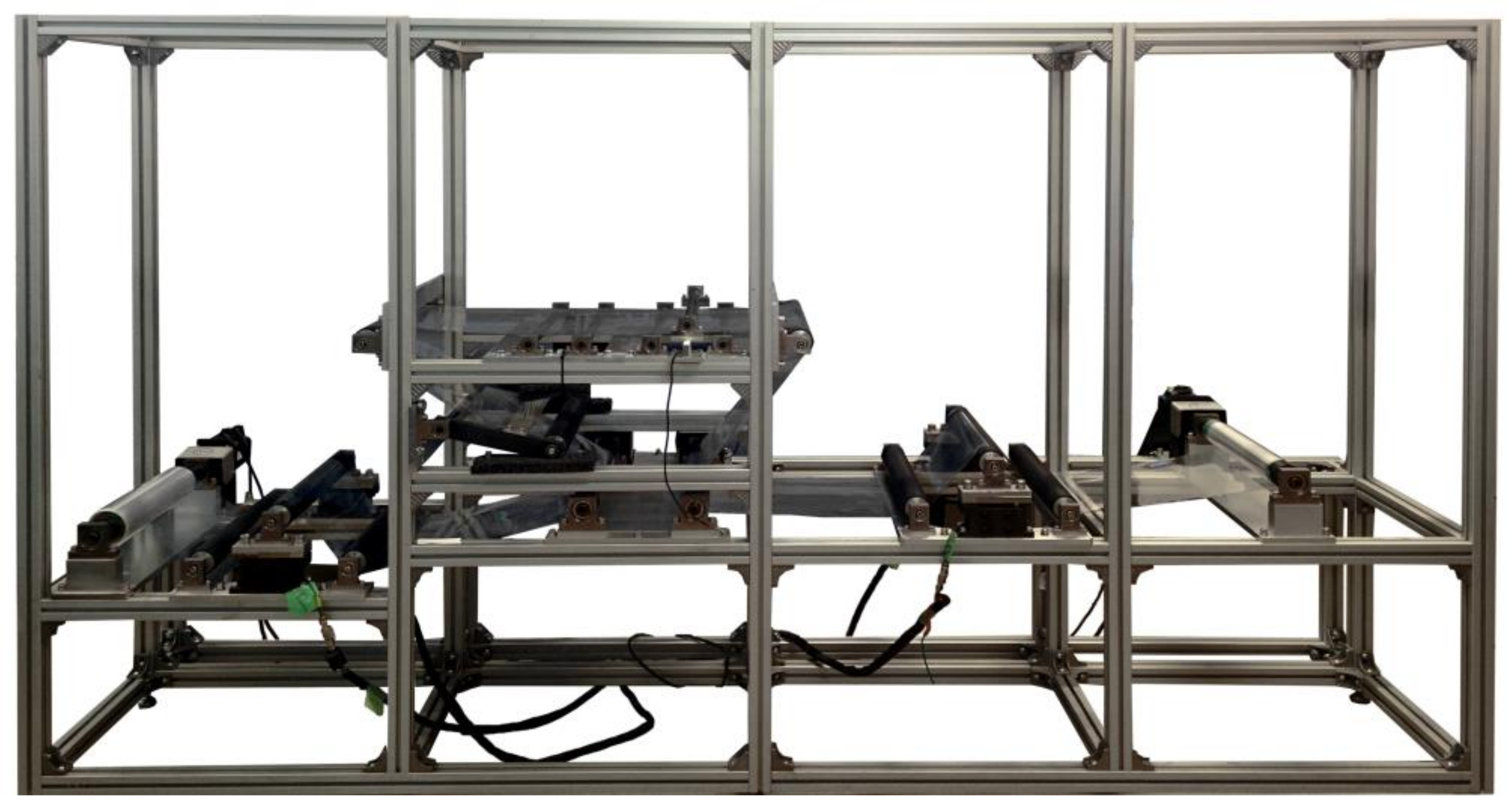
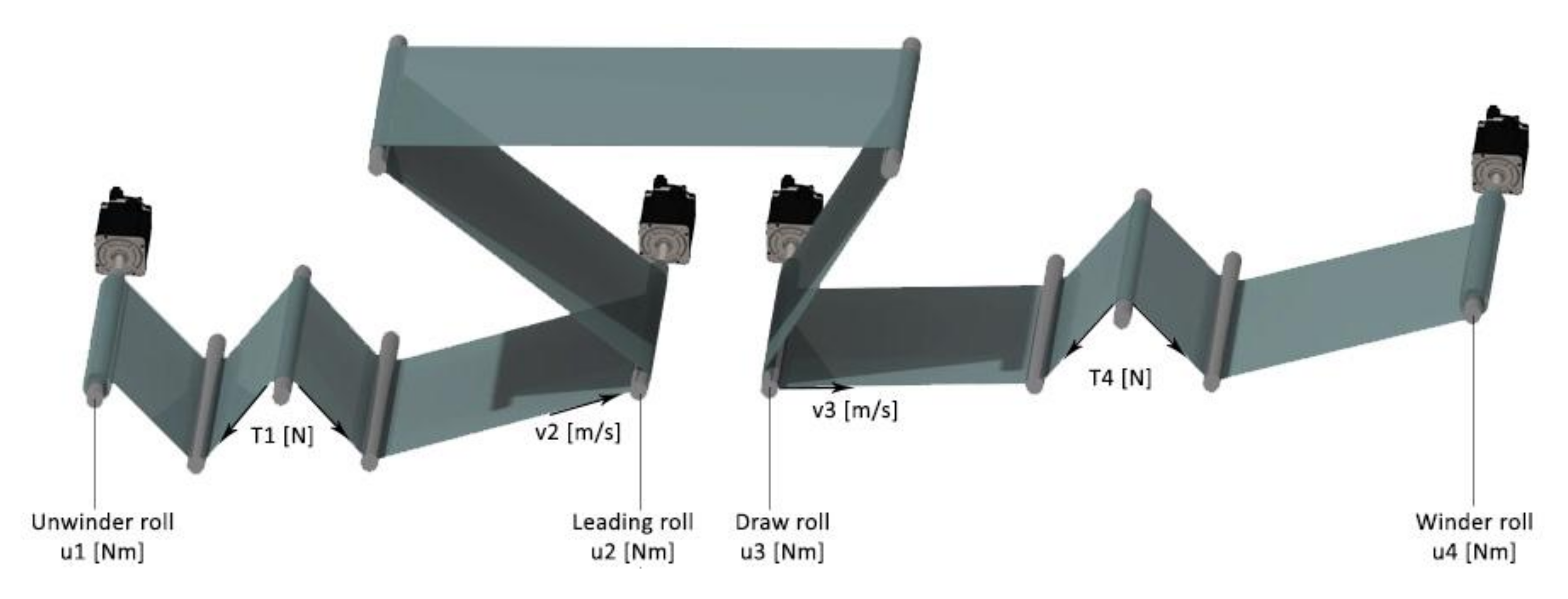
The realised system, developed in the last years and introduced in [22,23], comprises four main sections, each driven by one servomotor. The sections are strongly interlaced, and a total of 12 rolls, placed on a mechanical frame at different heights, make it up. The realised platform is intended to represent a large transport system similar to many industrial ones. The system was completely renewed at the end of 2015, with its performance improved by substituting all the rolls and their bearings with new ones (low weight and low friction). The platform is depicted in Figure 1, and a scheme is shown in Figure 2. The four servomotors that drive the transport system have 750 (W) of power 2.39 [Nm] of maximum torque. They are set in torque control mode by using an internal control of the servomotor to guarantee a precise force delivered to the system. The first servomotor is dedicated to the unwinder section, the second to the lead section, the third to the draw-roll section, the last to the winder section, as shown in Figure 2.

Two pairs of tension sensors (one for each side of the web) were placed after the unwinder roll (first pair of tension sensors) and before the winder roll (second pair of tension sensors). The first pair of tension sensors was followed by a pair of guide rolls (lead section) wrapped to maximize the contact area between the web and the drive rolls, reducing the possibility of slippage between the web and the rolls during the web transport.

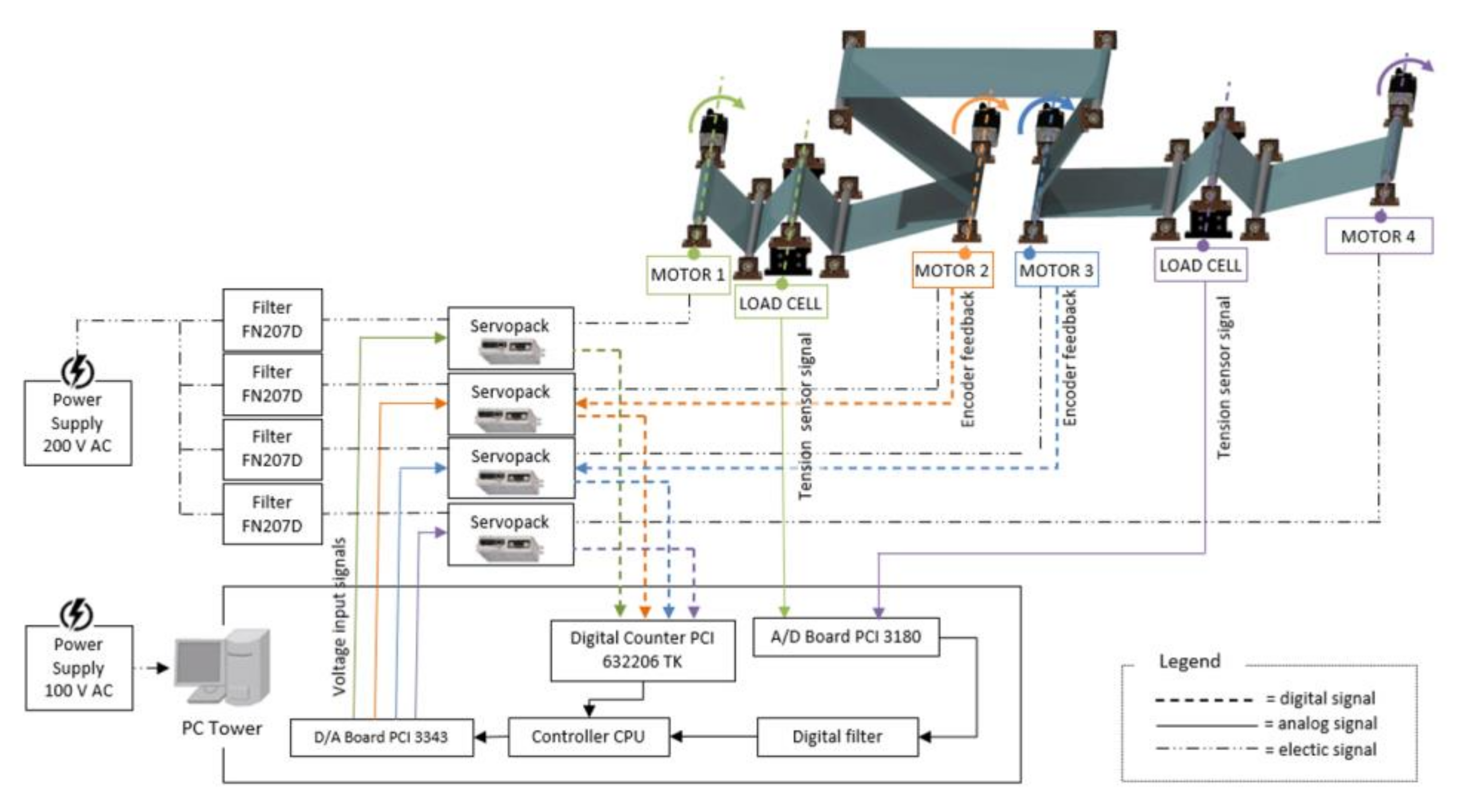
The servomotors were driven by voltage input signals of Ui, i = 1, …, 4, which, in torque control mode, are proportional to the torques that the motors exert on the corresponding roller. The tension sensor signals related to the unwinder roll and the winder roll were acquired by the A/D board, considering the average value of the two corresponding sides for measuring the tension after the unwinder (T₁) and before the winder (T₄). The four motor encoder signals fed a digital counter: in the proposed identification strategy, the speed of the lead section (v₂) and the draw-roll section (v₃) are the control variables. The controller’s CPU receives signals through A/D boards and counters, performs the control algorithm and generates the command signals in real-time, driving the servomotors via D/A boards with a sampling time of 0.01 [s]. Moreover, a set of filtering circuits was inserted; they were hardware filter banks (model FN270D) connected to the servo packs driving the four motors. Moreover, a digital moving average filter was applied to the acquired data.

A functional diagram of the transport line indicating the four servomotors (type SGMAS 08ACA21), their driving servo packs, CPU controller, analogue (A/D Board PCI 3180) and digital (Digital Counter PCI 632206 TK) acquisition boards, sensors, filters banks (type FN207D), their connections (electrical, digital and analogue signals) and power supply is shown in Figure 3.

As depicted in Figure 1, the whole system was mounted on a mechanical frame designed to support the system’s components. Each of the four motors was connected to the respective roller using specific low-friction connection joints. The power cables were placed far away concerning the signal cables, and all the cables were covered with insulating tape. The system comprises four drive rolls divided into three sections with lengths named L₁, L₂, and L₃. The [8] geometric and mass properties of the four drive rolls are shown in

Table 1. Description of the physical properties of the platform.

Section	Symbol	Value
UNWINDER
Radius	r1	3.26 × 10−2 [m]
Moment of Inertia	J1	4.42 × 10−3 [kg m2]
Span of the section	L1	0.75 [m]
LEADING
Radius	r2	2.5 × 10−2 [m]
Moment of Inertia	J2	6.10 × 10−3 [kg m2]
Span of the section	L2	1.2 [m]
DRAW ROLL
Radius	r3	1.5 × 10−2 [m]
Moment of Inertia	J3	6.1 × 10−3 [kg m2]
Span of the section	L3	1.25 [m]
WINDER
Radius	r4	3.22 × 10−2 [m]
Moment of Inertia	J4	4.39 × 10−3 [kg m2]

.

Table 2. Physical properties of the OPP film.

Properties	Symbol	Value
Width	w	0.3 [m]
Thickness	Th	40 [μ]
Cross-sectional area	A	1.2 × 10−5 [m2]
Density	ρ	910 [kg/m3]
Young modulus	E	9.8 × 109 [N/m2]
Tensile strength	σR	32 × 106 [N/m2]
Yield strength	σY	22 × 106 [N/m2]
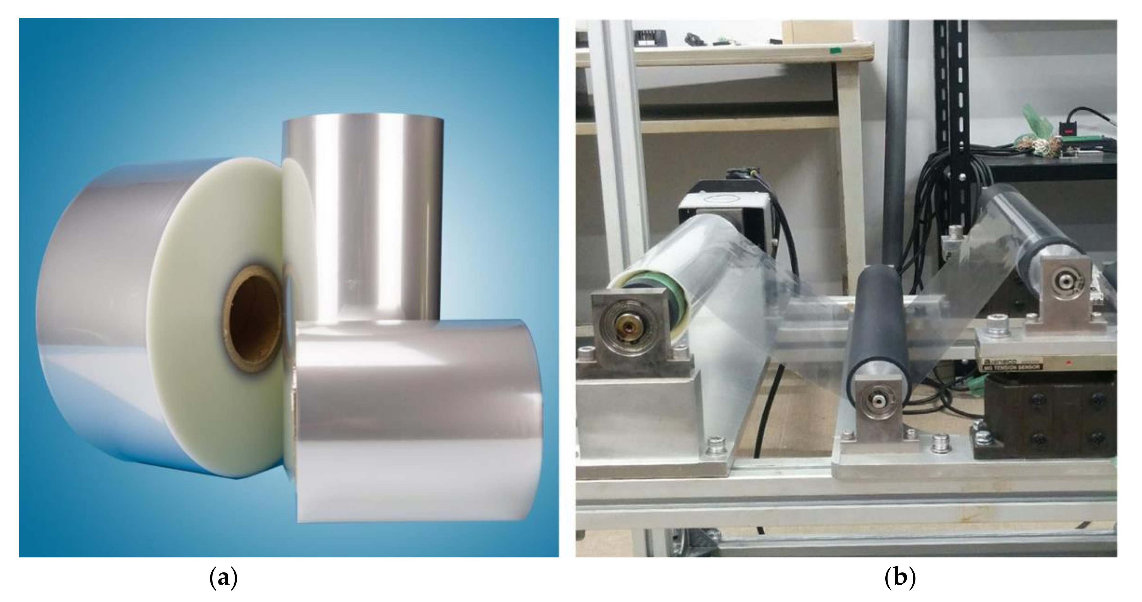
Viscosity coefficient	η	1.5 × 109 [Ns/m2]

sums up the main material properties of the Bi-Oriented Polypropylene (OPP) film used in the experimental web handling system, and Figure 4 shows a stock image of the film roll (a) and the rolls mounting on the experimental system (b).

2.1. Lumped Model for the Experimental Web Tension Control System

The model of the web transport systems is based on three laws applied at each section between two consecutive rolls [1]:

-

Conservation of mass: the law of conservation of mass for the web section for evaluating the relationship between the speeds of two adjacent rolls and the strain in the web;

-

Torque balance: the angular velocity of the k_th roll can be obtained through a torque balance as a function of the tension forces T_k+1 and T_k applied to the roll from the web;

-

Voigt model: for taking into account the linear viscoelasticity of web-material expressed as a combination of linear springs and dampers, the Voigt model was considered.

The torque balance equation is expressed in Equation (1) for the generic k_th section. J_k and r_k are respectively the total inertia and the roll’s radius of the k_th roll, u_k is the motor torque applied at the k_th roll, C_k and k_fk are respectively the dry friction torque and the viscous friction coefficient. The conservation of mass equation is expressed in Equation (2) for the k_th and k_th+1 section with longitudinal velocities v_k and v_k+1 where ε is elasticity coefficient, and L_k is the length between the k_th and the k_th+1 roll. The Voigt model equation is shown in Equation (3), where σ_k is the stress applied at the k_th section, E is the material Young’s modulus, η is the material viscosity coefficient.

$$\frac{d\left(J_k·{\omega }_k\right)}{dt}=r_k·\left(T_{k+1}-T_{k+1}\right)+u_k-C_k-k_{fk}·{\omega }_k$$

(1)

$$\epsilon =\frac{1}{L_k}·\int (v_{k+1}-v_k)dt$$

(2)

$${\sigma }_k=E·\epsilon +\eta ·\frac{d\epsilon }{dt}$$

(3)

Equations (1)–(3) may be applied for each of the four sections of the system and then transformed in the Laplace domain considering starting conditions equal to 0 for tension force T_k and velocity ω_k of each k_th section. Substituting Equation (2) in Equation (3) in the Laplace domain, Equation (3) may be transformed in a relation between T_k(s) and ε(s) as expressed in Equation (4), where A is the web section area. The last equality of Equation (4) introduces a polynomial, named P(s), depending only on the physical characteristics of the web.

$$T_k\left(s\right)=A·\eta ·\left(\frac{1+\frac{\eta }{E}·s}{\frac{\eta }{E}·s}\right)·s·\epsilon \left(s\right)=P\left(s\right)·s·\epsilon \left(s\right)$$

(4)

Equation (1), transformed in the Laplace domain, permits the calculation of the longitudinal velocities v_k(s) for the k_th section; Equations (5)–(8) show the expression of the longitudinal velocities for the four sections of the considered platform, considering the orientation of the motor for determining the sign of the motor torque u_k applied to the k_th section.

$$v_1\left(s\right)=\frac{r_1}{s·J_1}·\left[T_1\left(s\right)·r_1-u_1\left(s\right)-C_1-k_{f1}·{\omega }_1\left(s\right)\right],$$

(5)

$$v_2\left(s\right)=\frac{r_2}{s·J_2}·\left[(T_2\left(s\right)-T_1\left(s\right))·r_2+u_2\left(s\right)-C_2-k_{f2}·{\omega }_2\left(s\right)\right] ,$$

(6)

$$v_3\left(s\right)=\frac{r_3}{s·J_3}·\left[(T_4\left(s\right)-T_2\left(s\right))·r_3+u_3\left(s\right)-C_3-k_{f3}·{\omega }_3\left(s\right)\right] ,$$

(7)

$$v_4\left(s\right)=\frac{r_4}{s·J_4}·\left[u_4\left(s\right)-T_4\left(s\right)·r_4-C_4-k_{f4}·{\omega }_4\left(s\right)\right] ,$$

(8)

The inputs of the system are the motor torque values u₁, u₂, u_3, u₄, the outputs of the system are the forces T₁ and T₄ and the longitudinal roll speed values are v₂ and v₃ of Section 2 and Section 3. Equations (5)–(8) may be integrated with the Voigt–Kelvin viscoelasticity law (Equation (5) applied at each section) allowing for the determination of the values of T₁, T₂ and T₄. It is not difficult to show how complex the system is, as interconnections exist between the input and outputs of the four subsystems [6,22].

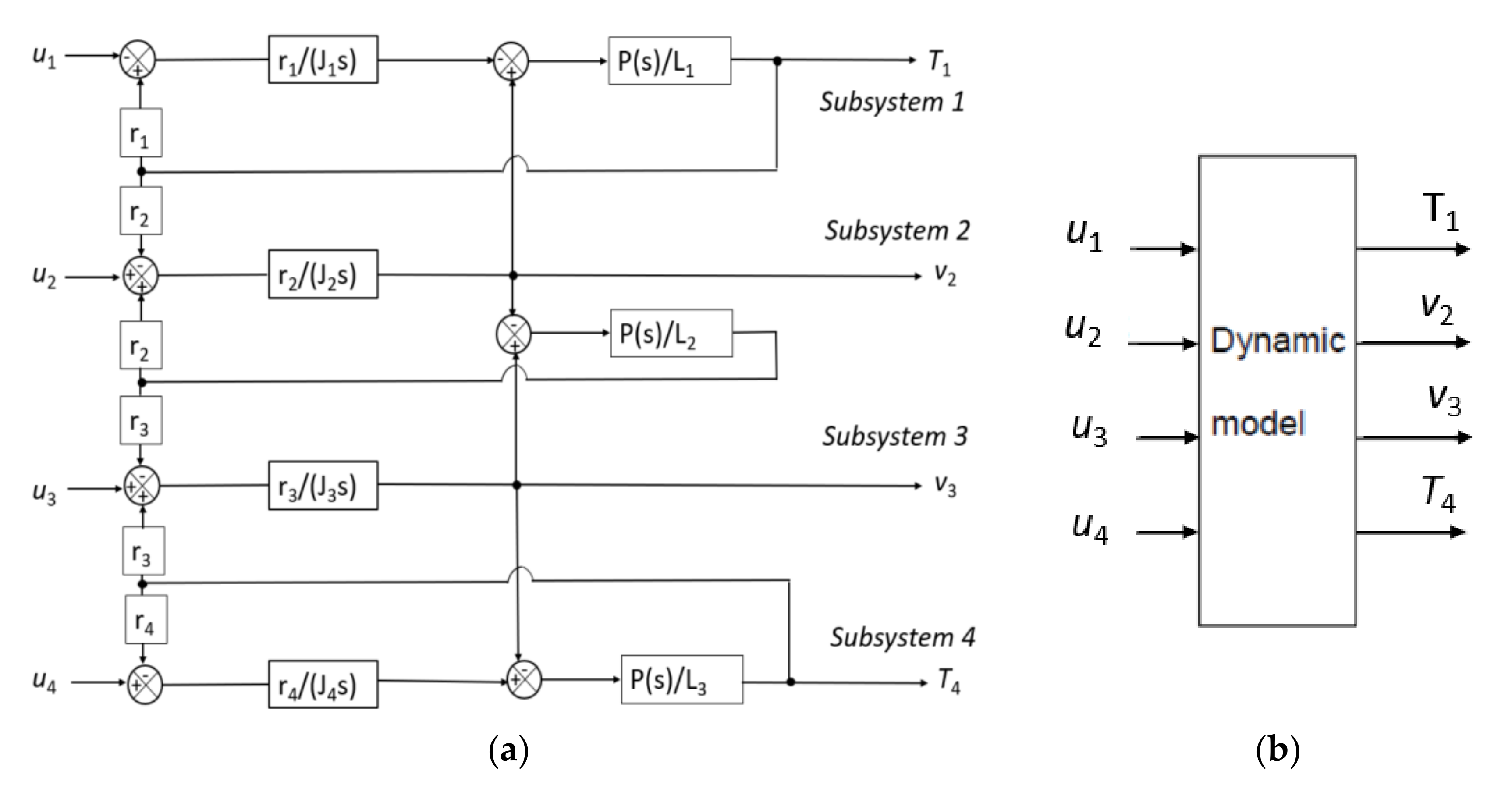
To have an idea of the structure of the mathematical physical model in a manner that simplifies Equations (5)–(8) by neglecting the frictional effects expressed by the coefficients C_k and k_fk, which are very difficult to estimate experimentally, the resulting model without frictional terms is shown in Figure 5a in the Laplace domain. The model structure shown in Figure 5a permits highlighting the inputs (u₁, u₂, u₃, u₄), the outputs (the forces T₁ and T₄ and the longitudinal roll speed v₂ and v₃) and the four subsystems corresponding to the system sections.

This type of mathematical description does not seem to be effective for the following reasons:

• There is no way to appreciate the interactions that affect the individual subsystems. This is a MIMO system, and each input influences individual outputs, as is clearly depicted in Figure 5a.
• The mathematical model used to describe the system’s behaviour cannot provide any indication of the value of the dissipative parameters; if not appropriately identified, viscous friction coefficients make the mathematical model wrong and unable to describe the reality of the physical phenomenon.
• It is impossible to study the system’s stability in any way and to predict its behaviour by varying the operating conditions. Most control techniques require formulating the problem as a “transfer function” to control and operate on the poles and zeros that characterise the system considered.

For all these reasons, a new approach was proposed to analyse the problem considering exclusively a direct identification of the dynamical MIMO model shown in Figure 5b based on the experimental data obtained evaluating the inputs and outputs of the system.

2.2. Development of a Procedure for Model Identification

The input–output relation of the system model shown in Figure 5b is expressed with input u₁, u₂, u₃, u₄ and output T₁, v₂, v₃, T₄ and may be expressed in a generic form with 16 transfer functions G_ij as expressed in Equation (9):

$$\left(\begin{array}{c}{T}_1\\ v_2\\ \begin{array}{c}{v}_3\\ T_4\end{array}\end{array}\right)=\left(\begin{array}{c}\begin{array}{ccc}{G}_{11}& G_{12}& \begin{array}{cc}{G}_{13}& G_{14}\end{array}\end{array}\\ \begin{array}{ccc}{G}_{21}& G_{22}& \begin{array}{cc}{G}_{23}& G_{24}\end{array}\end{array}\\ \begin{array}{c}\begin{array}{ccc}{G}_{31}& G_{32}& \begin{array}{cc}{G}_{33}& G_{34}\end{array}\end{array}\\ \begin{array}{ccc}{G}_{41}& G_{42}& \begin{array}{cc}{G}_{43}& G_{44}\end{array}\end{array}\end{array}\end{array}\right)·\left(\begin{array}{c}{u}_1\\ \begin{array}{c}{u}_2\\ \begin{array}{c}{u}_3\\ u_4\end{array}\end{array}\end{array}\right)$$

(9)

The procedure here proposed for model identification considers that for a system such as the one analysed, the MIMO model Equation (9) includes transfer functions that, for the physical constitution of the system, have a different weight and importance for the system behaviour. In particular, the extra-diagonal transfer functions referring to the effects of the external subsystems on the i_th subsystem may be considered an uncertainty of the estimation procedure, a disturbance leading to a model constituted by 4 SISO systems, which are characterised by the estimated SISO transfer functions G_ii^e. The estimated identified simplified model is expressed by Equation (10).

$$\left(\begin{array}{c}{T}_1\\ v_2\\ \begin{array}{c}{v}_3\\ T_4\end{array}\end{array}\right)=\left(\begin{array}{c}\begin{array}{ccc}{G}_{11}^e& 0& \begin{array}{cc}0& 0\end{array}\end{array}\\ \begin{array}{ccc}0& G_{22}^e& \begin{array}{cc}0& 0\end{array}\end{array}\\ \begin{array}{c}\begin{array}{ccc}0& 0& \begin{array}{cc}{G}_{33}^e& 0\end{array}\end{array}\\ \begin{array}{ccc}0& 0& \begin{array}{cc}0& G_{44}^e\end{array}\end{array}\end{array}\end{array}\right)·\left(\begin{array}{c}{u}_1\\ \begin{array}{c}{u}_2\\ \begin{array}{c}{u}_3\\ u_4\end{array}\end{array}\end{array}\right)$$

(10)

2.3. Collecting Experimental Data for System Identification

Model identification requires a preliminary collection of input and output data from experimental tests. In this phase, it is important to demonstrate, through statistical inference methods, that the system outputs show a certain repeatable behaviour. When these conditions are satisfied, it is possible to accept such inputs to the bench machine.

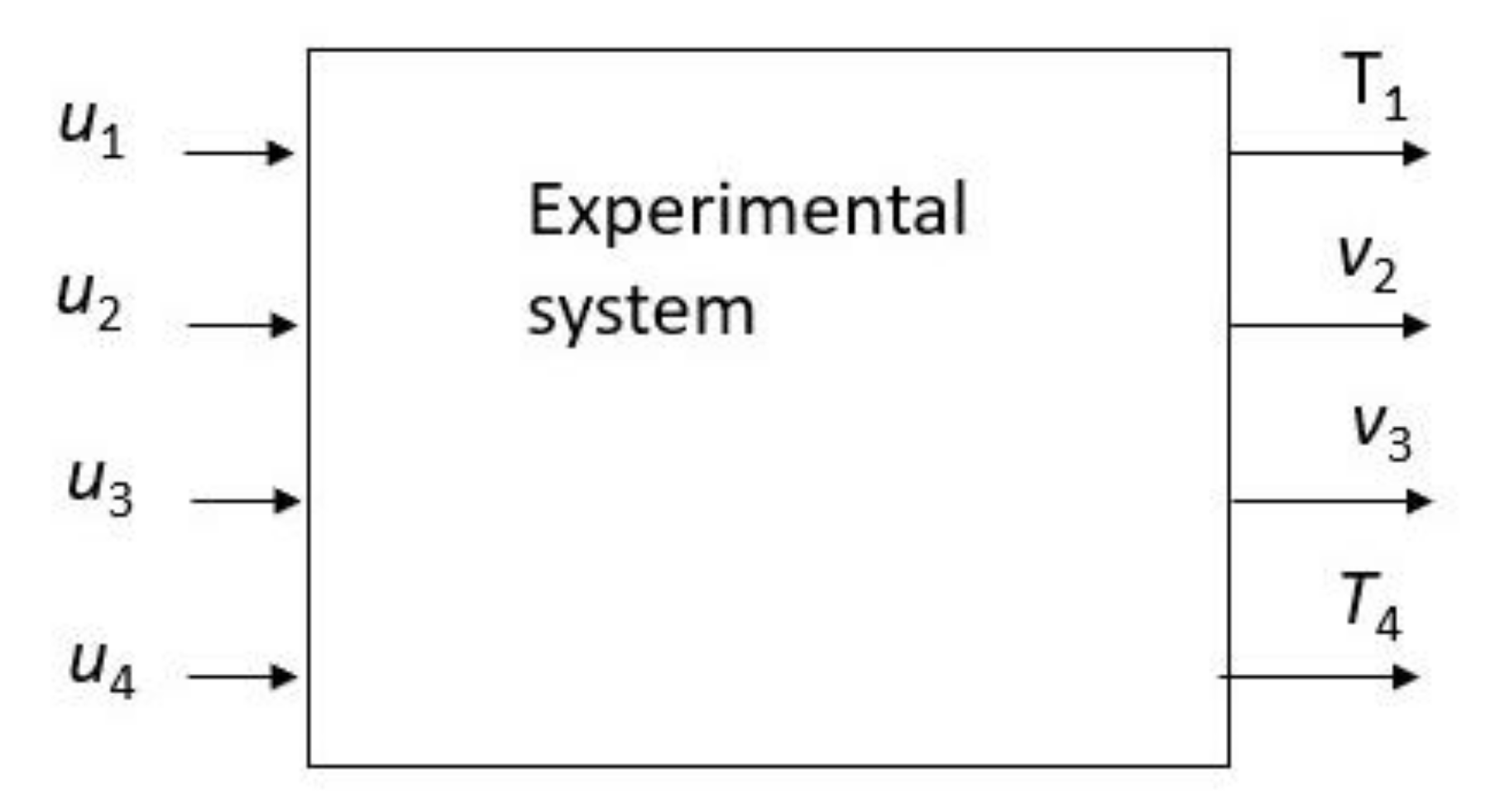
When the web tension platform works in an open loop, choosing appropriate servomotor voltage input values becomes important for the experimental campaign. Each motor of the system is set up for torque control modality, so that it is possible to set the values of voltage input signals (in Volts) for each servo motor. This information is converted in torque through the motor constant Kk = 0.8 [Nm/V], so that torque [Nm] = tension signal [V] x motor constant [Nm/V]. The block diagram of the open-loop tests is schematised in Figure 6.

The following sets of voltage inputs (

Table 3. Experimental test executed in open loop.

Name of Test	u1 [V]	u2 [V]	u3 [V]	u4 [V]
A	0.35	0.08	0.08	0.5
B	0.2	0.06	0.06	0.4
C	0.2	0.08	0.08	0.3
D	0.3	0.08	0.08	0.4
E	0.4	0.08	0.08	0.55
F	0.2	0.06	0.06	0.3
G	0.1	0.06	0.06	0.18

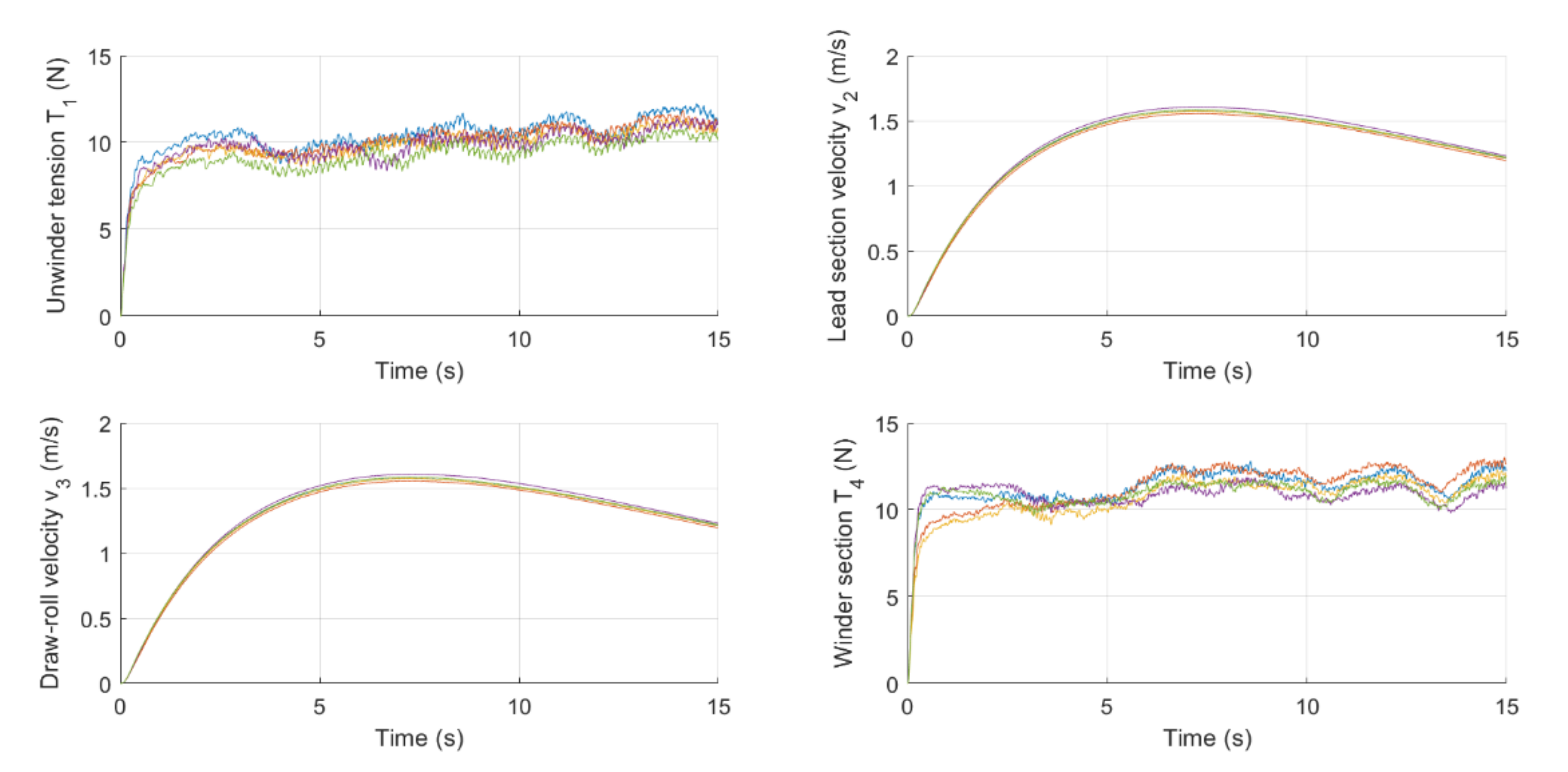
) were assigned respectively to unwinder, lead-section, draw-roll and winder servomotors (u₁, u₂, u₃, u₄). For each combination of inputs, five tests were carried out to have detailed information about the statistical repeatability of the tests.

The five repetitions of every test show a similar trend: in Figure 7, the outputs (T₁, v₂, v₃, T₄) of five repetitions of Test E (Table 3). The temporal length of all the tests was 15 s.

The proposed identification procedure is based on a complete routine developed in the Matlab environment (using the System Identification Toolbox app) [21] with an integrated graphical user interface that permits the user first to import the data of the experimental tests to be analysed. All the different repetitions of the same test are used to identify and validate the model, making the validation more reliable. The following step consists of estimating the transfer function models; it is necessary to define the number of poles, the number of zeros and, eventually, the delay. 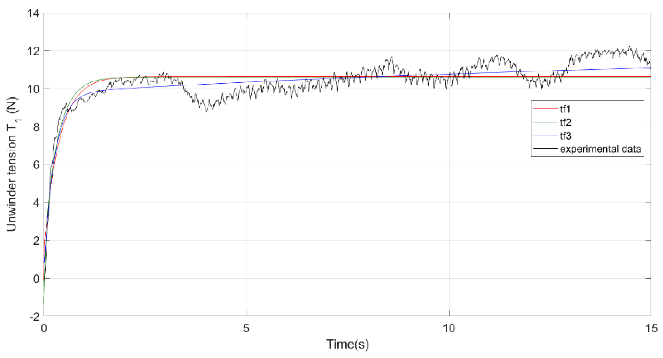Using the System Identification Toolbox app [21] makes it possible to compare with the same experimental data different types of transfer functions, having different combinations of zeros, poles and delay. In Figure 8, the comparison of three different estimated transfer functions (tf1, tf2 and tf3) with the experimental data referred to T₁ in one of the five repetitions for Test E. The transfer functions shown in Figure 8 have respectively 2 poles, 1 zero, 0.1 delay (tf1), 2 poles, 0 zeros, 0 delay (tf2) and 2 poles, 0 zeros and 0.1 delay for tf3.

3. Results

In the industrial application of system identification, an important objective is often to obtain the least complex model within the limits of the required model accuracy. In our case, after a few attempts, an optimal number of parameters was determined for web platform system identification: 2 poles, 1 zero and 0 delays for all the transfer functions to estimate $G_{11}^e$, $G_{22}^e$, $G_{33}^e$, $G_{44}^e$ The realised routine, after loading the experimental data of the considered test, permits the insertion of the characteristics of the transfer functions to estimate the number of poles, number of zeros and delay, and then estimates the transfer functions, explaining the estimated poles, zeros and delays and, finally, produces a comparative plot between the experimental data related to the variables T₁, v₂, v₃ and T₄ and the same variables obtained by the estimated transfer functions with the same input of the experimental data, also giving an index of performance in the percentage of the similarity of behaviours. Figure 9 shows the identification results for the first repetition of Test E (in all the Figures of the manuscript, T₁ and T₄ are expressed in Newton and v₂ and v₃ in m/s), and the poles and zeros of the estimated transfer functions are reported in

Table 4. Poles and zeros of the estimated transfer functions (first repetition Test E), 2 poles, 1 zero.

Transfer Function	Zero	Pole 1	Pole 2
$G_{11}^e$	−0.0146	−4.2833	0
$G_{22}^e$	−0.0158	−0.2194	−0.1041
$G_{33}^e$	−0.0162	−0.2185	−0.1053
$G_{44}^e$	−0.2666	−5.8543	−0.1943

.

The poles and zeros are properties of the transfer function and, therefore, the differential equation describing the input–output system dynamics. They characterise the differential equation and provide a complete description of the system, including interesting information about the system stability.

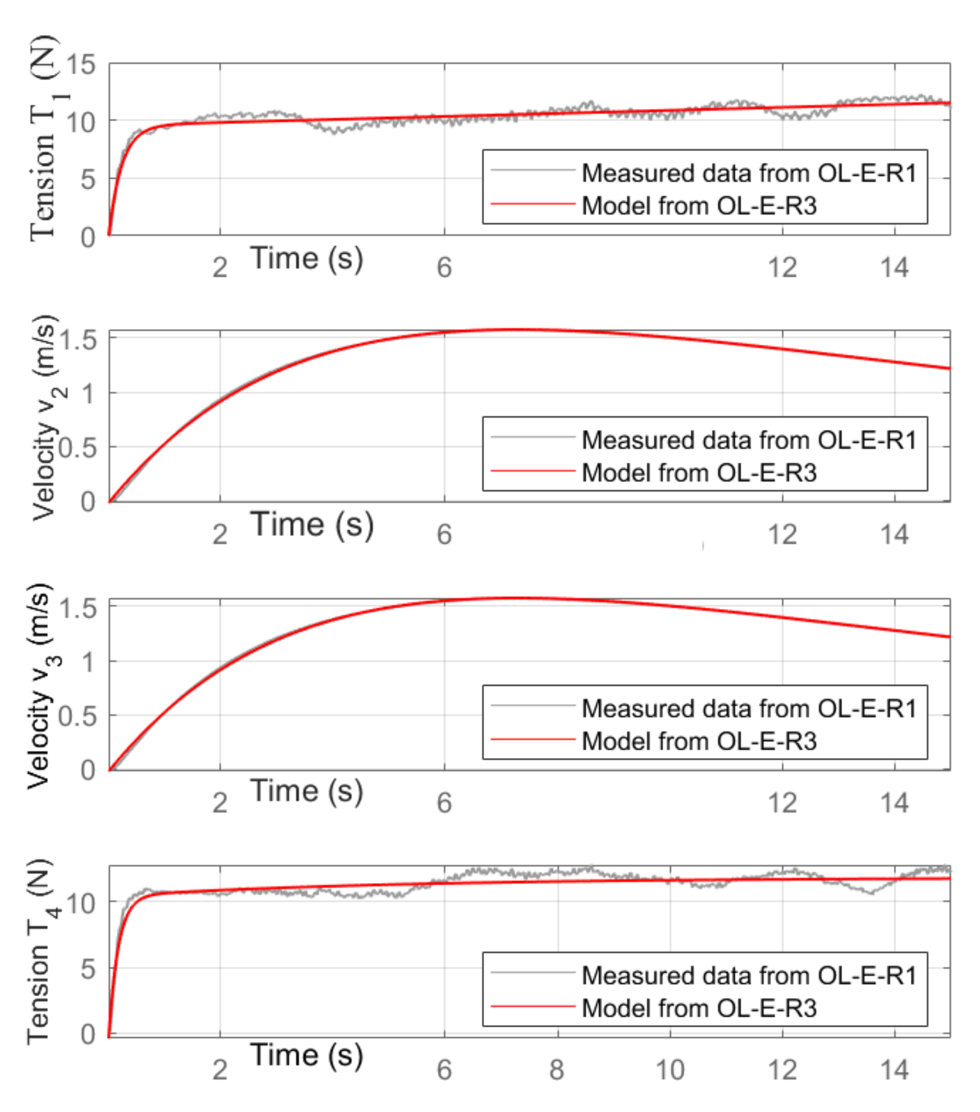
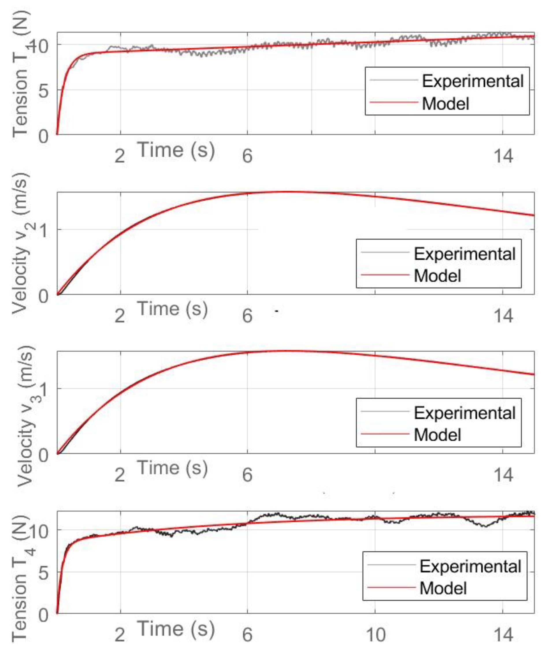
Moreover, the estimated model was validated using a different repetition of a test in the same condition used for identification. Figure 10 shows the validation results obtained comparing the simulated response from Repetition 3 of Test E (named E-OL-R3) and the experimental response from Test E Repetition 1 (OL-E-R1). It is evident, also considering the performance parameter, that the transfer functions estimated from E-OL-R3 overlap very well with the experimental data of another test (OL-E-R1), validating the proposed procedure with different repetitions of the same combination of inputs.

System Simulation Using the Measured Input

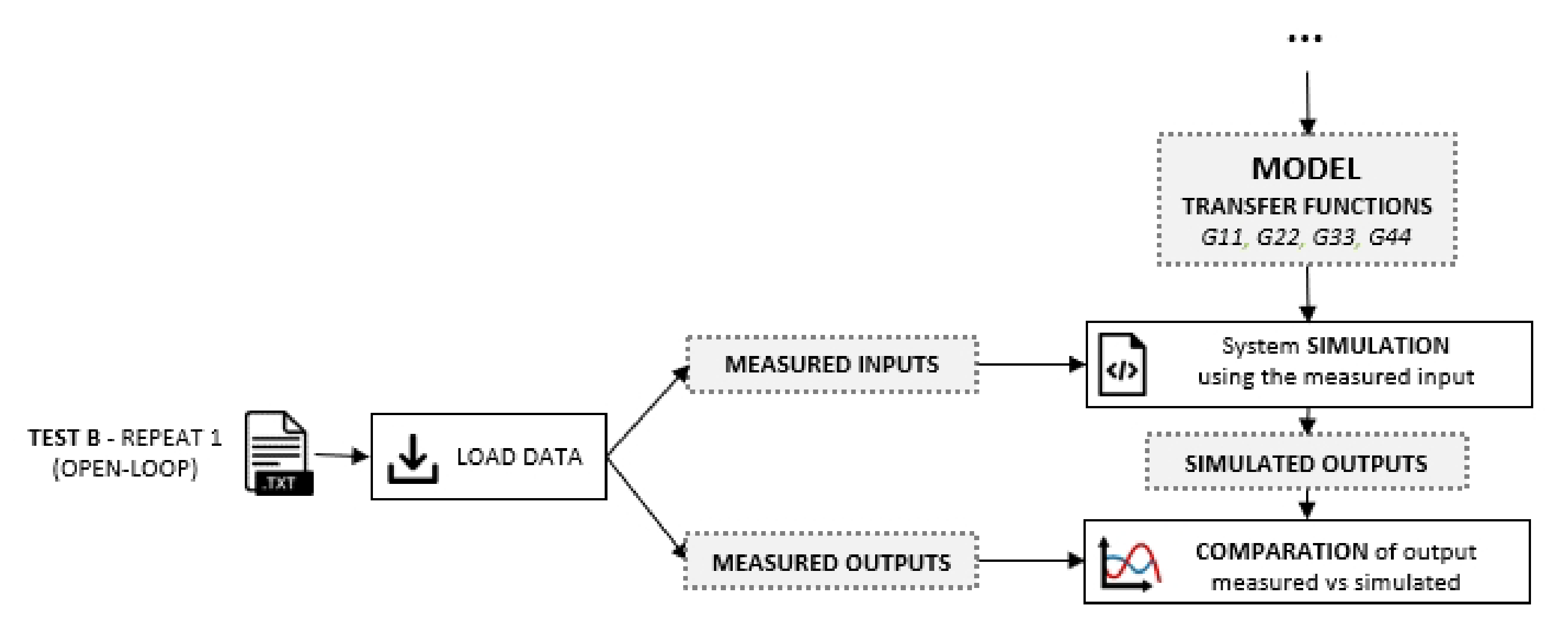
The purpose of the proposed procedure is to verify that the estimated model fulfils the modelling requirements according to subjective and objective criteria of good model approximation. The model of the system estimated can be used to simulate the system’s behaviour with a certain combination of torque to the motors, different from those used for the estimation. The outputs simulated can be compared with the measured ones to validate the model in different conditions. If this comparison gives good results, then it is possible to predict the system’s behaviour, during both the transient and the steady state, at a work point different from the one of identification. The validation procedure is explained in the diagram shown in Figure 11, where a generic open-loop experimental test (i.e., Test B Repetition 1 as indicated in Figure 11, referring to the terminology in Table 3) is loaded. The measured outputs (the variables T₁, v₂, v₃, T₄) are compared with the simulated outputs obtained by the model identified from a different test (i.e., Test E) and then analysed with the same input used for the experimental data. If this comparison gives good results, it is possible to predict the system’s behaviour, during both the transient and the steady state, at a work point different from the one of identification.

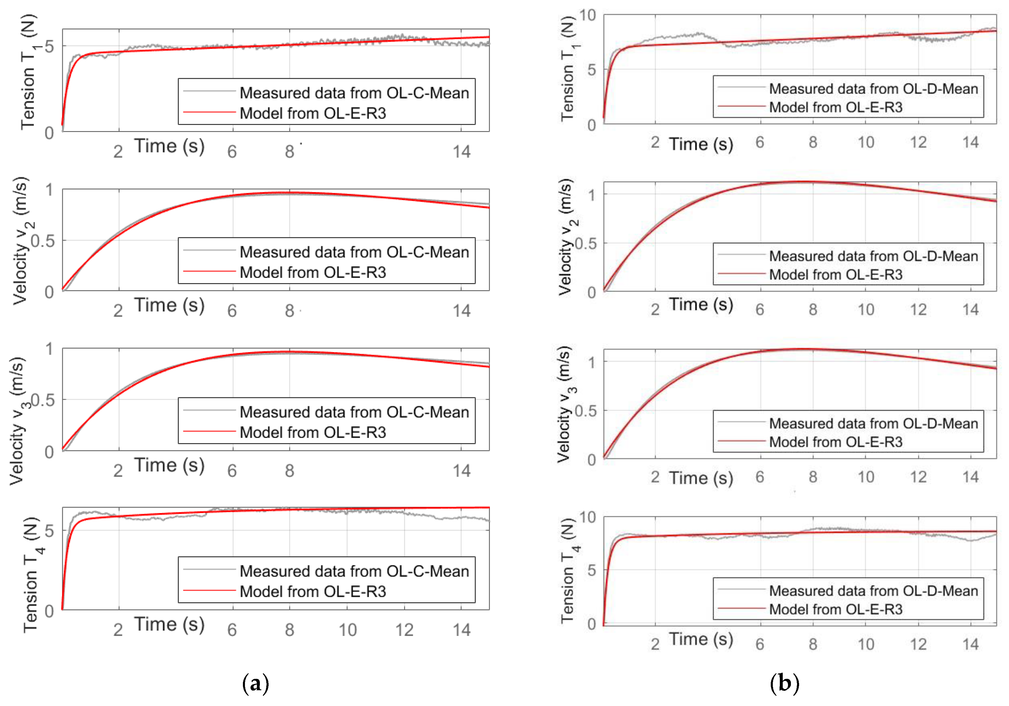
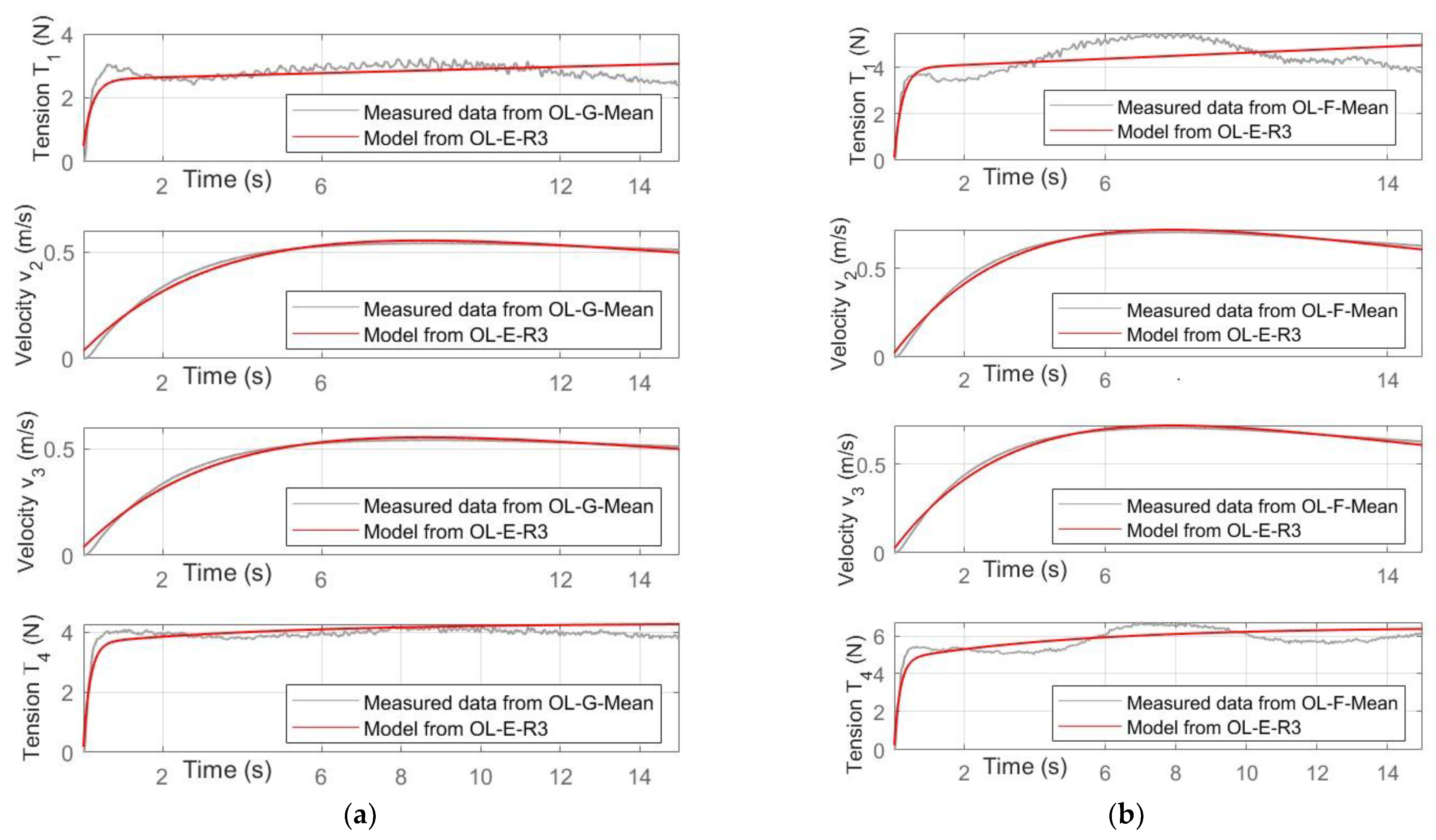
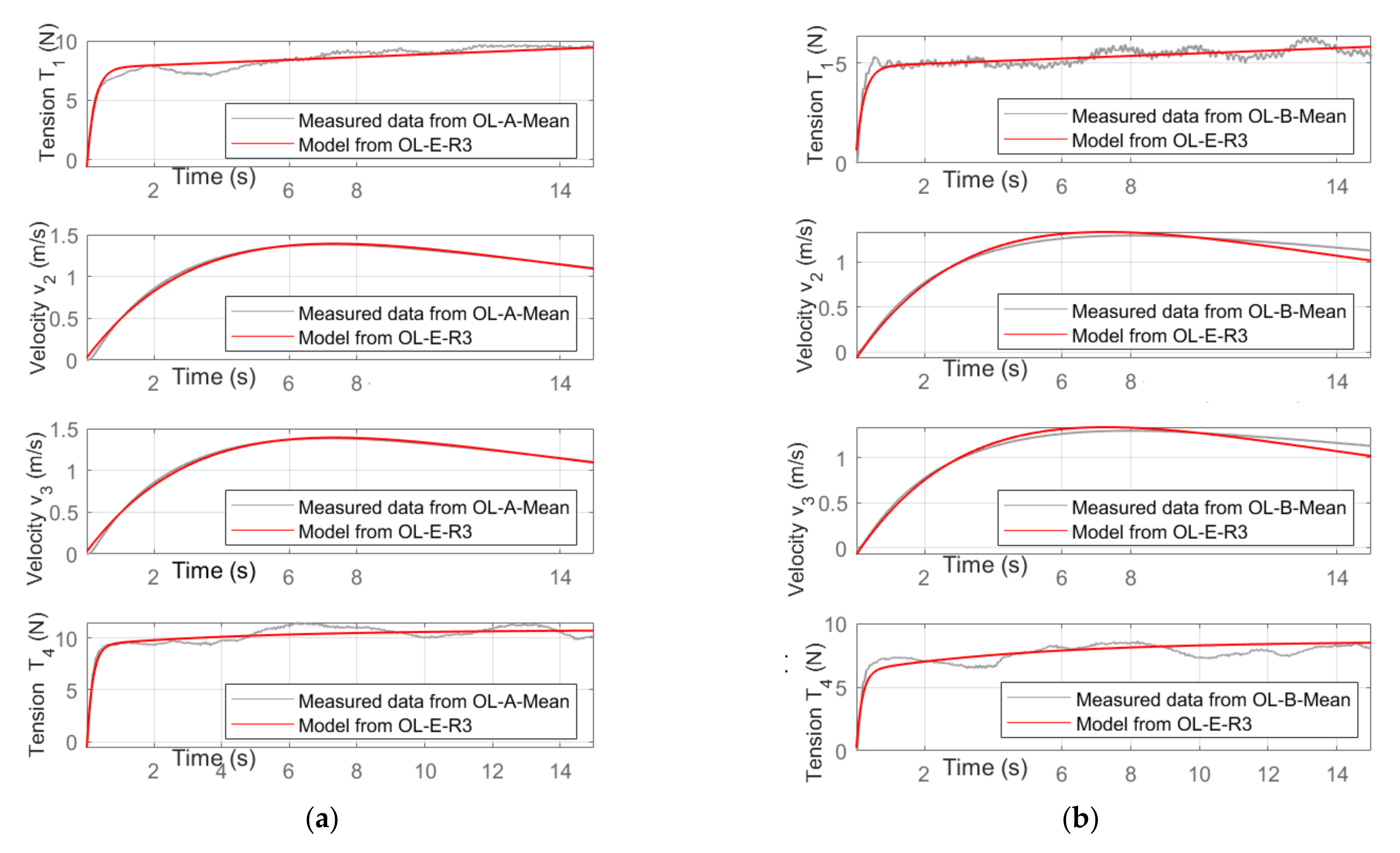
The comparison was carried out for all the experimental tests indicated in Table 3; for each combination of input, the average of the five repetitions was considered, and the identified model was obtained from Test E (Repetition 3). The results are depicted in Figure 12, Figure 13 and Figure 14, where the validations with the tests A, B, C, D, F and G are shown for each control variable of each test.

The results illustrated in Figure 12, Figure 13 and Figure 14 clearly show that the model identified by a single experimental test with a specific combination of inputs (third repetition of typology E) has good behaviour even for different and various combinations of inputs that vary in an extended range. The performance indicator of the comparison always assumes very high values (close to 100%) for the speed v₂ and v₃, while it assumes somewhat lower values for the voltages T₁ and T₄. However, by analysing all the corresponding diagrams, it can be noted that the difference between the experimental trends of T₁ and T₄ and those generated by the simple model proposed is mainly due to the fluctuations of the experimental values, which may depend on various factors and measurement errors. It can therefore be concluded that the model obtained with the proposed methodology is inserted in the variability field of the same repetitions (see Figure 7) and allows, in all the input combinations analysed, for predicting with good accuracy the behaviour of the complex experimental platform. Considering that the proposed identification and modelling procedure does not need the implementation of any equation, as illustrated above, but only some preliminary experimental tests, it is believed that it may be useful for industrial applications, even complex ones, in which the identification of a sufficiently accurate model must be made quickly and easily.

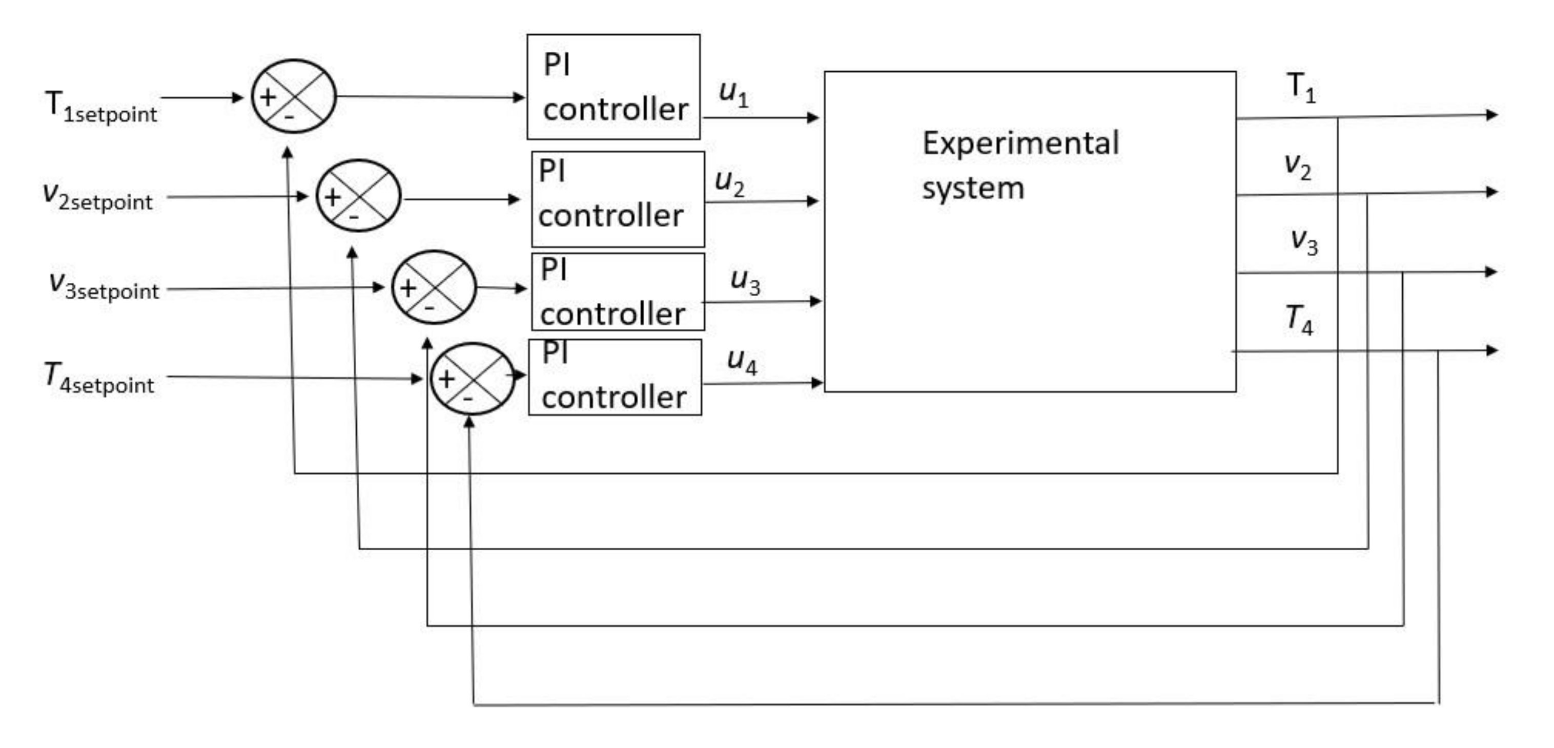
Finally, to test the identified model’s performance in the Identification for Control (I4C) target, the identified model was used by completing a closed-loop model in Simulink environment [24] with a classical PI controller applied for each of the four subsystems. The scheme of the experimental test in the closed loop is shown in Figure 15, and the feedback is ensured by the tension sensors (T₁ and T₄) and by the servomotor encoders (v₂ and v₃).

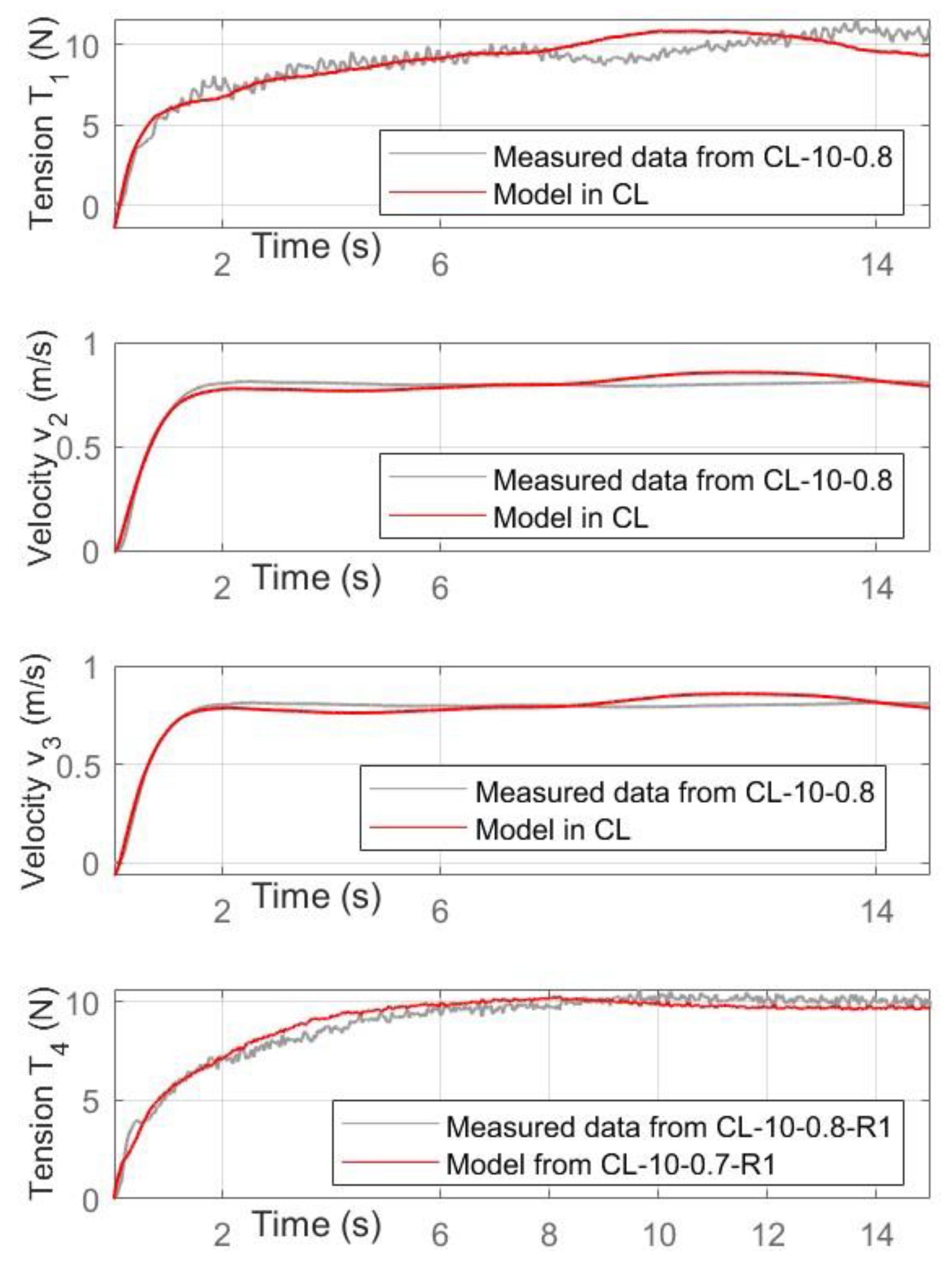
In Figure 16, the comparison is between the experimental data and the data from the identified model with a target value for the PI controller equal to 10 Newton for T₁ and T₄ (T_1setpoint and T_4setpoint in Figure 15) and 0.8 m/s for v₂ and v₃ (v_2setpoint and v_3setpoint in Figure 15). The comparison in Figure 16 shows a good correlation between the experimental data and the prediction of the identified model. Similar results were carried out with other experimental tests in the closed loop.

4. Discussion and Conclusions

This work shows how a MIMO experimental web handling system can be identified through simple transfer functions, composed of a few parameters, in the Identification for control (I4C) perspective. The model of the system is estimated in Section 3, using the data of a single test (Test E Repetition 3) in an open loop, allows for simulating the system’s behaviour with step inputs in a wide range of operations. The validation depicted in Figure 12, Figure 13 and Figure 14 demonstrates that the identified model can describe the experimental behaviour of the web transport platform from a steady-state velocity of about 0.5 m/s (Tests G) to the velocity of about 1.4 m/s (Tests A). Therefore, it is possible to predict the system’s behaviour, during both the transient and the steady state, with a certain combination of torque to the motors. Therefore, once the model’s validity in a certain field of operation is verified, the application becomes a powerful tool to carry out an unlimited number of tests, acting on different degrees of freedom and observing the variations in the system’s response. There is a need to underline the extreme simplicity of the procedure and the absence of any complex system of equations to solve, which is different from the classical approach for modelling this kind of system.

Using the MATLAB Simulink environment [17], the estimated model simulated the closed-loop system’s operation. The developed application allows for changing the reference set-points to impose and modify the controller parameters, i.e., the gains of the PI regulators and the smoothing constant of the reference signal. Therefore, once the model’s validity in a certain field of operation is verified, the application becomes a powerful tool to conduct simulated tests, acting on different degrees of freedom and observing variation in the system’s response.

Simulating numerous tests in the same conditions as those performed in the laboratory and comparing the simulated and measured data, it was found that, as for the open loop, even the estimated model in this case provides a good approximation of the behaviour of the system, as long as the operative conditions do not change significantly from the point of operation of the test used for identification. As a possible future development, it is suggested that a more complex system model be implemented with parameters that depend on the work point. However, it is not required to act in a wide field of operation in most cases, so that this safe methodology has great chances for industrial applications, which often demand fixed work points.

In the future, an application that performs tuning of the controller could be implemented, which, once the model is identified and set-points are chosen, establishes the gains that allow for reaching the set-points quickly but without any overshoots that could damage the web.