Global Picture of Genetic Relatedness and the Evolution of Humankind

 ,
,  ,
,
Simple Summary
Abstract
1. Introduction
2. Results
2.1. IBD Statistics
2.2. Modern Genomes
2.3. Ancient Genomes
2.4. Time Periods for IBD Sharing between Populations
3. Discussion
3.1. Problems with Short IBDs and Estimation Their Time of Origin
3.2. Modern Genomes
3.3. Ancient Genomes
4. Conclusions
5. Materials and Methods
- IAB is the number of IBD fragments per pair of individuals from populations A and B;
- NA is the normalization coefficient for population A from the HeatMapTable (last row);
- NB is the normalization coefficient for population B from the HeatMapTable (last row);
- JAB is the normalized IAB value.
Supplementary Materials
Author Contributions
Funding
Acknowledgments
Conflicts of Interest
References
- Fedorova, L.; Qiu, S.; Dutta, R.; Fedorov, A. Atlas of Cryptic Genetic Relatedness among 1000 Human Genomes. Genome Biol. Evol. 2016, 8, 777–790. [Google Scholar] [CrossRef] [PubMed]
- NCBI. Available online: https://ftp.ncbi.nlm.nih.gov/snp/latest_release/release_notes.txt (accessed on 9 November 2020).
- Schiffels, S.; Durbin, R. Inferring Human Population Size and Separation History from Multiple Genome Sequences. Nat. Genet. 2014, 46, 919–925. [Google Scholar] [CrossRef] [PubMed]
- Pagani, L.; Lawson, D.J.; Jagoda, E.; Mörseburg, A.; Eriksson, A.; Mitt, M.; Clemente, F.; Hudjashov, G.; DeGiorgio, M.; Saag, L.; et al. Genomic Analyses Inform on Migration Events During the Peopling of Eurasia. Nature 2016, 538, 238–242. [Google Scholar] [CrossRef]
- Wall, J.D.; Ratan, A.; Stawiski, E.; Kim, H.L.; Kim, C.; Gupta, R.; Suryamohan, K.; Gusareva, E.S.; Purbojati, R.W.; Bhangale, T.; et al. Identification of African-Specific Admixture between Modern and Archaic Humans. Am. J. Hum. Genet. 2019, 105, 1254–1261. [Google Scholar] [CrossRef] [PubMed]
- Conomos, M.P.; Reiner, A.P.; Weir, B.S.; Thornton, T.A. Model-free Estimation of Recent Genetic Relatedness. Am. J. Hum. Genet. 2016, 98, 127–148. [Google Scholar] [CrossRef] [PubMed]
- The 1000 Genomes Project Consortium A Global Reference for Human Genetic Variation. Nature 2015, 526, 68–74. [CrossRef]
- Mallick, S.; Li, H.; Lipson, M.; Mathieson, I.; Gymrek, M.; Racimo, F.; Zhao, M.; Chennagiri, N.; Nordenfelt, S.; Tandon, A.; et al. The Simons Genome Diversity Project: 300 Genomes from 142 Diverse Populations. Nature 2016, 538, 201–206. [Google Scholar] [CrossRef]
- Bergström, A.; McCarthy, S.A.; Hui, R.; Almarri, M.A.; Ayub, Q.; Danecek, P.; Chen, Y.; Felkel, S.; Hallast, P.; Kamm, J.; et al. Insights Into Human Genetic Variation and Population History From 929 Diverse Genomes. Science 2020, 367, 5012. [Google Scholar] [CrossRef]
- Genome Asia100K Consortium. The GenomeAsia 100K Project Enables Genetic Discoveries Across Asia. Nature 2019, 576, 106–111. [Google Scholar] [CrossRef]
- Carmi, S.; Hui, K.Y.; Kochav, E.; Liu, X.; Xue, J.; Grady, F.; Guha, S.; Upadhyay, K.; Ben-Avraham, D.; Mukherjee, S.; et al. Sequencing an Ashkenazi Reference Panel Supports Population-Targeted Personal Genomics and Illuminates Jewish and European Origins. Nat. Commun. 2014, 5, 4835. [Google Scholar] [CrossRef]
- Turro, E. Whole-Genome Sequencing of Patients with Rare Diseases in a National Health System. Nature 2020, 583, 96–102. [Google Scholar] [CrossRef] [PubMed]
- Skov, L.; Macià, M.C.; Sveinbjörnsson, G.; Mafessoni, F.; Lucotte, E.A.; Einarsdóttir, M.S.; Jonsson, H.; Halldorsson, B.; Gudbjartsson, D.F.; Helgason, A.; et al. The Nature of Neanderthal Introgression Revealed by 27,566 Icelandic Genomes. Nature 2020, 582, 78–83. [Google Scholar] [CrossRef] [PubMed]
- Oleksyk, T.K.; Brukhin, V.; O’Brien, S. The Genome Russia Project: Closing the Largest Remaining Omission on the World Genome Map. GigaScience 2015, 4, 53. [Google Scholar] [CrossRef] [PubMed]
- David Reich Lab at Harvard. Available online: https://reich.hms.harvard.edu/datasets (accessed on 9 November 2020).
- Lao, O.; Lu, T.T.; Nothnagel, M.; Junge, O.; Freitag-Wolf, S.; Caliebe, A.; Balascakova, M.; Bertranpetit, J.; Bindoff, L.A.; Comas, D.; et al. Correlation between Genetic and Geographic Structure in Europe. Curr. Biol. 2008, 18, 1241–1248. [Google Scholar] [CrossRef]
- Sankararaman, S.; Mallick, S.; Dannemann, M.; Prüfer, K.; Kelso, J.; Pääbo, S.; Patterson, N.; Reich, D. The Genomic Landscape of Neanderthal Ancestry in Present-Day Humans. Nature 2014, 507, 354–357. [Google Scholar] [CrossRef]
- Meyer, M.; Kircher, M.; Gansauge, M.-T.; Li, H.; Racimo, F.; Mallick, S.; Schraiber, J.G.; Jay, F.; Prüfer, K.; De Filippo, C.; et al. A High-Coverage Genome Sequence from an Archaic Denisovan Individual. Science 2012, 338, 222–226. [Google Scholar] [CrossRef]
- Qin, P.; Stoneking, M. Denisovan Ancestry in East Eurasian and Native American Populations. Mol. Biol. Evol. 2015, 32, 2665–2674. [Google Scholar] [CrossRef]
- Sankararaman, S.; Mallick, S.; Patterson, N.; Reich, D. The Combined Landscape of Denisovan and Neanderthal Ancestry in Present-Day Humans. Curr. Biol. 2016, 26, 1241–1247. [Google Scholar] [CrossRef]
- Akkuratov, E.E.; Gelfand, M.S.; Khrameeva, E.E. Neanderthal and Denisovan Ancestry in Papuans: A Functional Study. J. Bioinform. Comput. Biol. 2018, 16, 1840011. [Google Scholar] [CrossRef]
- Wong, E.H.; Khrunin, A.; Nichols, L.; Pushkarev, D.; Khokhrin, D.; Verbenko, D.A.; Evgrafov, O.; Knowles, J.; Novembre, J.; Limborska, S.; et al. Reconstructing Genetic History of Siberian and Northeastern European Populations. Genome Res. 2016, 27, 1–14. [Google Scholar] [CrossRef]
- Sikora, M.; Pitulko, V.V.; Sousa, V.C.; Allentoft, M.E.; Vinner, L.; Rasmussen, S.; Margaryan, A.; Damgaard, P.D.B.; De La Fuente, C.; Renaud, G.; et al. The Population History of Northeastern Siberia Since the Pleistocene. Nature 2019, 570, 182–188. [Google Scholar] [CrossRef] [PubMed]
- Lazaridis, I.; Patterson, N.; Mittnik, A.; Renaud, G.; Mallick, S.; Kirsanow, K.; Sudmant, P.H.; Schraiber, J.G.; Castellano, S.; Lipson, M.; et al. Ancient Human Genomes Suggest Three Ancestral Populations for Present-Day Europeans. Nature 2014, 513, 409–413. [Google Scholar] [CrossRef] [PubMed]
- Mathieson, I.; Alpaslan-Roodenberg, S.; Posth, C.; Szécsényi-Nagy, A.; Rohland, N.; Mallick, S.; Olalde, I.; Broomandkhoshbacht, N.; Candilio, F.; Cheronet, O.; et al. The Genomic History of Southeastern Europe. Nature 2018, 555, 197–203. [Google Scholar] [CrossRef] [PubMed]
- Povysil, G.; Hochreiter, S. IBD Sharing between Africans, Neandertals, and Denisovans. Genome Biol. Evol. 2016, 8, 3406–3416. [Google Scholar] [CrossRef]
- Browning, S.R. Estimation of Pairwise Identity by Descent from Dense Genetic Marker Data in a Population Sample of Haplotypes. Genetics 2008, 178, 2123–2132. [Google Scholar] [CrossRef]
- Smith, G.R.; Nambiar, M. New Solutions to Old Problems: Molecular Mechanisms of Meiotic Crossover Control. Trends Genet. 2020, 36, 337–346. [Google Scholar] [CrossRef]
- Cavalli-Sforza, L.L.; Menozzi, P.; Piazza, A. The History and Geography of Human Genes; Princeton University Press: Princeton, NJ, USA, 2018. [Google Scholar]
- Wang, C.-C.; Reinhold, S.; Kalmykov, A.; Wissgott, A.; Brandt, G.; Jeong, C.; Cheronet, O.; Ferry, M.; Harney, E.; Keating, D.; et al. Ancient Human Genome-Wide Data From a 3000-Year Interval in the Caucasus Corresponds with Eco-Geographic Regions. Nat. Commun. 2019, 10, 590. [Google Scholar] [CrossRef]
- Nielsen, R.; Akey, J.M.; Jakobsson, M.; Pritchard, J.K.; Tishkoff, S.; Willerslev, R.N.E. Tracing the Peopling of the World Through Genomics. Nature 2017, 541, 302–310. [Google Scholar] [CrossRef]
- Tambets, K.; Yunusbayev, B.; Hudjashov, G.; Ilumäe, A.-M.; Rootsi, S.; Honkola, T.; Vesakoski, O.; Atkinson, Q.; Skoglund, P.; Kushniarevich, A.; et al. Genes Reveal Traces of Common Recent Demographic History for Most of the Uralic-Speaking Populations. Genome Biol. 2018, 19, 139. [Google Scholar] [CrossRef]
- Hanak, P.; Sugar, P.F.; Frank, T. (Eds.) A History of Hungary; Indiana University Press: Bloomington, IN, USA, 1990. [Google Scholar]
- Raghavan, M.; Steinrücken, M.; Harris, K.; Schiffels, S.; Rasmussen, S.; DeGiorgio, M.; Albrechtsen, A.; Valdiosera, C.; Ávila-Arcos, M.C.; Malaspinas, A.-S.; et al. Genomic Evidence for the Pleistocene and Recent Population History of Native Americans. Science 2015, 349, aab3884. [Google Scholar] [CrossRef]
- Skoglund, P.; Mallick, S.; Bortolini, M.C.; Chennagiri, N.; Hünemeier, T.; Petzl-Erler, M.L.; Salzano, F.M.; Patterson, N.; Reich, D. Genetic Evidence for Two Founding Populations of the Americas. Nature 2015, 525, 104–108. [Google Scholar] [CrossRef] [PubMed]
- Tishkoff, S.A.; Reed, F.A.; Friedlaender, F.R.; Ehret, C.; Ranciaro, A.; Froment, A.; Hirbo, J.B.; Awomoyi, A.A.; Bodo, J.-M.; Doumbo, O.; et al. The Genetic Structure and History of Africans and African Americans. Science 2009, 324, 1035–1044. [Google Scholar] [CrossRef] [PubMed]
- Fan, S.; Kelly, D.E.; Beltrame, M.H.; Hansen, M.E.B.; Mallick, S.; Ranciaro, A.; Hirbo, J.; Thompson, S.; Beggs, W.; Nyambo, T.; et al. African Evolutionary History Inferred From Whole Genome Sequence Data of 44 Indigenous African Populations. Genome Biol. 2019, 20, 82. [Google Scholar] [CrossRef] [PubMed]
- Tucci, S.; Akey, J.M. The Long Walk to African Genomics. Genome Biol. 2019, 20, 1–3. [Google Scholar] [CrossRef] [PubMed]
- Dryomov, S.V.; Nazhmidenova, A.M.; Shalaurova, S.A.; Morozov, I.V.; Tabarev, A.V.; Starikovskaya, E.B.; Sukernik, R.I. Mitochondrial Genome Diversity at the Bering Strait Area Highlights Prehistoric Human Migrations From Siberia to Northern North America. Eur. J. Hum. Genet. 2015, 23, 1399–1404. [Google Scholar] [CrossRef]
- Reich, D.; Patterson, N.; Kircher, M.; Delfin, F.; Nandineni, M.R.; Pugach, I.; Ko, A.M.-S.; Ko, Y.-C.; Jinam, T.A.; Phipps, M.E.; et al. Denisova Admixture and the First Modern Human Dispersals into Southeast Asia and Oceania. Am. J. Hum. Genet. 2011, 89, 516–528. [Google Scholar] [CrossRef]
- Jacobs, G.S.; Hudjashov, G.; Saag, L.; Kusuma, P.; Darusallam, C.C.; Lawson, D.J.; Mondal, M.; Pagani, L.; Ricaut, F.-X.; Stoneking, M.; et al. Multiple Deeply Divergent Denisovan Ancestries in Papuans. Cell 2019, 177, 1010–1021.e32. [Google Scholar] [CrossRef]
- Browning, S.R.; Browning, B.L.; Zhou, Y.; Tucci, S.; Akey, J.M. Analysis of Human Sequence Data Reveals Two Pulses of Archaic Denisovan Admixture. Cell 2018, 173, 53–61. [Google Scholar] [CrossRef]
- Chen, L.; Wolf, A.B.; Fu, W.; Li, L.; Akey, J.M. Identifying and Interpreting Apparent Neanderthal Ancestry in African Individuals. Cell 2020, 180, 677–687. [Google Scholar] [CrossRef]
- Durvasula, A.; Sankararaman, S. Recovering Signals of Ghost Archaic Introgression in African Populations. Sci. Adv. 2020, 6, 5097. [Google Scholar] [CrossRef]
- Andrews, S. FastQC: A Quality Control Tool for High Throughput Sequence Data. 2010. Available online: http://www.bioinformatics.babraham.ac.uk/projects/fastqc (accessed on 9 November 2020).
- Li, H.; Durbin, R. Fast and Accurate Short Read Alignment with Burrows-Wheeler Transform. Bioinformatics 2009, 25, 1754–1760. [Google Scholar] [CrossRef] [PubMed]
- Li, H.; Handsaker, B.; Wysoker, A.; Fennell, T.; Ruan, J.; Homer, N.; Marth, G.; Abecasis, G.; Durbin, R. The Sequence Alignment/Map Format and SAM Tools. Bioinformatics 2009, 25, 2078–2079. [Google Scholar] [CrossRef] [PubMed]
- Pedersen, B.S.; Quinlan, A.R. Mosdepth: Quick Coverage Calculation for Genomes and Exomes. Bioinformatics 2017, 34, 867–868. [Google Scholar] [CrossRef] [PubMed]
- Garrison, E. Haplotype-Based Variant Detection from Short-Read Sequencing. arXiv 2012, arXiv:1207.3907 [q-bio.GN]. Available online: https://arxiv.org/abs/1207.3907 (accessed on 9 November 2020).
- Tan, A.; Abecasis, G.R.; Kang, H.M. Unified Representation of Genetic Variants. Bioinformatics 2015, 31, 2202–2204. [Google Scholar] [CrossRef] [PubMed]
- Danecek, P.; Auton, A.; Abecasis, G.; Albers, C.A.; Banks, E.; Depristo, M.A.; Handsaker, R.E.; Lunter, G.; Marth, G.T.; Sherry, S.T.; et al. The Variant Call Format and VCF Tools. Bioinformatics 2011, 27, 2156–2158. [Google Scholar] [CrossRef]
- Cingolani, P.; Patel, V.M.; Coon, M.; Nguyen, T.; Land, S.J.; Ruden, D.M.; Lu, X. Using Drosophila melanogaster as a Model for Genotoxic Chemical Mutational Studies with a New Program, SnpSift. Front. Genet. 2012, 3, 35. [Google Scholar] [CrossRef]
- Prüfer, K.; Racimo, F.; Patterson, N.; Jay, F.; Sankararaman, S.; Sawyer, S.; Heinze, A.; Renaud, G.; Sudmant, P.H.; De Filippo, C.; et al. The Complete Genome Sequence of a Neanderthal From the Altai Mountains. Nature 2014, 505, 43–49. [Google Scholar] [CrossRef]
- Mafessoni, F.; Grote, S.; De Filippo, C.; Slon, V.; Kolobova, K.A.; Viola, B.; Markin, S.V.; Chintalapati, M.; Peyrégne, S.; Skov, L.; et al. A high-Coverage Neandertal Genome from Chagyrskaya Cave. Proc. Natl. Acad. Sci. USA 2020, 117, 15132–15136. [Google Scholar] [CrossRef]
- Prüfer, K.; De Filippo, C.; Grote, S.; Mafessoni, F.; Korlević, P.; Hajdinjak, M.; Vernot, B.; Skov, L.; Hsieh, P.; Peyrégne, S.; et al. A High-Coverage Neandertal Genome from Vindija Cave in Croatia. Science 2017, 358, 655–658. [Google Scholar] [CrossRef]
- Fu, Q.; Li, H.; Moorjani, P.; Jay, F.; Slepchenko, S.M.; Bondarev, A.A.; Johnson, P.L.F.; Aximu-Petri, A.; Prüfer, K.; De Filippo, C.; et al. Genome Sequence of a 45,000-Year-Old Modern Human From Western Siberia. Nature 2014, 514, 445–449. [Google Scholar] [CrossRef] [PubMed]
- Mukiza, T.O.; Protacio, R.U.; Davidson, M.K.; Steiner, W.W.; Wahls, W.P. Diverse DNA Sequence Motifs Activate Meiotic Recombination Hotspots Through a Common Chromatin Remodeling Pathway. Genetics 2019, 213, 789–803. [Google Scholar] [CrossRef] [PubMed]
- R Core Team. R: A Language and Environment for Statistical Computing. 2018. Available online: https://www.r-project.org/ (accessed on 13 February 2012).
- Ignatov, D.I.; Poelmans, J.; Dedene, G.; Viaene, S. A New Cross-Validation Technique to Evaluate Quality of Recommender Systems. In Computer Vision; Springer Science and Business Media LLC: Berlin/Heidelberg, Germany, 2012; Volume 7143, pp. 195–202. [Google Scholar]


| Identifiers | Populations | Studied Populations from Americas | |||||||||||||||
|---|---|---|---|---|---|---|---|---|---|---|---|---|---|---|---|---|---|
| Cac | Cha | CLM | Col | Kar | May | Mix | MXL | PEL | Pia | Pim | PUR | Que | Sur | Wic | Zap | ||
| Cac_AMR | Cachi_Argentina | 53.5 | 4.5 | 1.3 | 59.3 | 3.8 | 6.7 | 6.0 | 2.7 | 4.3 | 8.3 | 5.4 | 1.1 | 30.3 | 9.0 | 9.2 | 5.2 |
| Cha_AMR | S_Chane:Argentina | 5.3 | N/A | 0.8 | 9.1 | 13.7 | 12.3 | 11.8 | 2.8 | 4.8 | 24.8 | 6.8 | 0.6 | 9.0 | 19.8 | 80.8 | 10.6 |
| CLM_AMR | Colombians_Medellin_Colombia | 1.2 | 0.7 | 25.6 | 1.0 | 0.9 | 0.8 | 1.8 | 12.0 | 8.3 | 1.2 | 0.9 | 12.7 | 1.2 | 0.8 | 0.6 | 1.9 |
| Col_AMR | Colla_Argentina | 60.6 | 7.8 | 1.0 | 86.1 | 6.2 | 6.2 | 6.2 | 2.4 | 4.3 | 6.7 | 6.7 | 0.6 | 31.6 | 6.2 | 10.1 | 6.1 |
| Kar_AMR | B_Karitiana:Brazil | 4.4 | 14.2 | 1.1 | 6.2 | 154.5 | 9.5 | 8.2 | 2.5 | 4.3 | 16.3 | 4.9 | 0.5 | 7.3 | 66.9 | 6.7 | 7.1 |
| May_AMR | S_Mayan:Mexico | 7.1 | 11.5 | 1.0 | 6.6 | 9.8 | 42.9 | 19.4 | 4.9 | 5.9 | 13.2 | 17.2 | 0.9 | 11.8 | 11.2 | 5.9 | 20.9 |
| Mix_AMR | B_Mixe:Mexico | 6.5 | 12.4 | 1.9 | 6.5 | 8.3 | 20.2 | 65.7 | 6.2 | 5.2 | 10.9 | 17.2 | 1.5 | 8.7 | 7.9 | 6.7 | 41.1 |
| MXL_AMR | Mexican_Ancestry_Los_Angeles | 2.2 | 1.9 | 11.9 | 2.1 | 1.9 | 3.5 | 4.1 | 17.6 | 11.2 | 2.4 | 3.8 | 10.7 | 1.8 | 2.2 | 2.0 | 5.9 |
| PEL_AMR | Peruvians_Lima_Peru | 2.5 | 2.6 | 8.0 | 2.6 | 3.2 | 4.0 | 3.5 | 10.5 | 18.3 | 3.1 | 3.4 | 6.9 | 5.0 | 2.4 | 2.2 | 4.5 |
| Pia_AMR | S_Piapoco:Colombia | 9.2 | 25.6 | 1.4 | 6.7 | 16.0 | 12.8 | 10.9 | 3.4 | 5.4 | 153.2 | 7.8 | 0.5 | 12.4 | 20.6 | 5.3 | 9.9 |
| Pim_AMR | S_Pima:Mexico | 5.4 | 8.3 | 1.1 | 7.3 | 5.1 | 18.3 | 17.3 | 6.2 | 5.3 | 8.9 | 168.9 | 0.3 | 9.8 | 8.5 | 7.1 | 17.1 |
| PUR_AMR | Puerto_Ricans_from_Puerto_Rico | 1.1 | 0.4 | 12.8 | 0.6 | 0.4 | 0.8 | 1.4 | 10.9 | 7.1 | 0.5 | 0.3 | 29.9 | 0.8 | 0.5 | 0.4 | 1.2 |
| Que_AMR | S_Quechua:Peru | 32.3 | 9.6 | 1.3 | 33.4 | 6.9 | 12.0 | 8.1 | 2.5 | 9.1 | 11.9 | 8.6 | 0.9 | 58.5 | 9.1 | 5.9 | 9.2 |
| Sur_AMR | S_Surui:Brazil | 9.9 | 21.5 | 0.8 | 6.2 | 65.9 | 11.2 | 8.2 | 2.8 | 4.2 | 21.0 | 8.9 | 0.6 | 8.8 | 153.2 | 7.0 | 9.5 |
| Wic_AMR | Wichi_Argentina | 9.6 | 80.3 | 0.6 | 10.2 | 6.3 | 5.7 | 6.2 | 2.7 | 3.5 | 5.3 | 6.9 | 0.4 | 5.9 | 6.8 | 236.9 | 10.2 |
| Zap_AMR | S_Zapotec:Mexico | 5.4 | 9.0 | 2.2 | 6.1 | 7.1 | 20.9 | 39.6 | 8.0 | 6.4 | 10.3 | 16.0 | 1.2 | 9.0 | 9.1 | 10.2 | 78.1 |
| Ale_ARC | S_Aleut:Russia | 1.0 | 0.8 | 2.7 | 1.4 | 3.2 | 4.8 | 2.3 | 3.3 | 2.4 | 3.7 | 4.7 | 2.3 | 2.5 | 4.1 | 2.0 | 2.5 |
| Chu_ARC | S_Chukchi:Russia | 0.8 | 0.7 | 1.3 | 0.6 | 1.1 | 1.6 | 1.7 | 1.6 | 1.1 | 0.6 | 2.2 | 1.3 | 0.6 | 0.8 | 0.8 | 0.9 |
| Esk_ARC | S_Eskimo_Sireniki:Russia | 1.3 | 2.7 | 0.4 | 1.1 | 1.8 | 2.2 | 2.5 | 1.5 | 1.6 | 2.2 | 5.5 | 0.4 | 1.8 | 1.9 | 1.8 | 3.1 |
| Ite_ARC | S_Itelman:Russia | 0.3 | 2.9 | 0.6 | 0.0 | 1.4 | 2.1 | 1.3 | 1.5 | 1.3 | 0.7 | 2.6 | 0.6 | 1.4 | 2.1 | 0.0 | 4.1 |
| Kor_ARC | Koryaks | 0.3 | 0.4 | 0.1 | 0.3 | 0.2 | 0.6 | 0.4 | 0.3 | 0.3 | 0.4 | 0.8 | 0.1 | 0.4 | 0.2 | 0.5 | 0.3 |
| Tli_ARC | S_Tlingit:Russia | 1.5 | 0.8 | 4.4 | 1.7 | 0.5 | 2.6 | 2.6 | 4.2 | 3.2 | 1.5 | 3.5 | 4.2 | 2.6 | 1.5 | 0.8 | 1.1 |
| Ulc_ARC | S_Ulchi:Russia | 0.6 | 0.7 | 0.3 | 0.7 | 0.4 | 1.7 | 0.4 | 0.9 | 1.0 | 0.0 | 0.9 | 0.2 | 0.2 | 0.7 | 0.2 | 1.7 |
| Alt_CAS | Altaian | 0.1 | 0.2 | 1.3 | 0.5 | 0.4 | 0.6 | 0.4 | 1.3 | 1.0 | 0.1 | 0.4 | 1.1 | 0.2 | 0.1 | 0.1 | 0.4 |
| Ish_CAS | Ishkasim_Tajikistan | 0.4 | 0.0 | 2.9 | 0.0 | 0.0 | 0.4 | 0.4 | 2.2 | 1.0 | 0.0 | 0.0 | 2.6 | 0.3 | 0.0 | 0.2 | 0.4 |
| Kal_CAS | Kalmyk | 0.4 | 1.8 | 1.1 | 0.5 | 1.8 | 0.0 | 0.0 | 1.1 | 0.9 | 0.0 | 0.0 | 1.1 | 0.6 | 0.0 | 0.0 | 0.9 |
| Kaz_CAS | Kazakhs_Kazakhstan | 0.3 | 0.0 | 1.9 | 0.3 | 0.2 | 0.0 | 0.2 | 1.4 | 0.8 | 0.3 | 0.0 | 1.7 | 0.0 | 0.0 | 0.2 | 0.3 |
| Kyr_CAS | S_Kyrgyz:Kyrgyzystan | 0.3 | 0.0 | 1.4 | 0.2 | 0.3 | 0.3 | 0.4 | 1.4 | 1.0 | 0.2 | 0.4 | 1.5 | 0.4 | 0.1 | 0.1 | 0.7 |
| Rus_CAS | Rushan-Vanch_Tajikistan | 0.2 | 0.0 | 3.4 | 0.2 | 0.0 | 0.0 | 0.6 | 2.6 | 2.3 | 0.4 | 0.7 | 3.3 | 0.6 | 0.0 | 0.2 | 0.0 |
| Shu_CAS | Shugnan_Tajikistan | 1.1 | 0.0 | 3.4 | 0.0 | 0.0 | 0.0 | 0.3 | 3.2 | 1.6 | 0.0 | 0.0 | 3.5 | 0.0 | 0.0 | 0.0 | 0.0 |
| Taj_CAS | Tajiks | 0.1 | 0.5 | 4.2 | 0.5 | 0.0 | 0.5 | 0.6 | 3.9 | 2.0 | 0.0 | 0.2 | 4.0 | 0.3 | 0.3 | 0.0 | 0.7 |
| TKm_CAS | Turkmens_Uzbekistan | 0.1 | 0.0 | 2.4 | 0.2 | 0.0 | 0.6 | 0.4 | 2.4 | 1.4 | 0.0 | 0.3 | 2.4 | 0.0 | 0.3 | 0.2 | 0.8 |
| Uyg_CAS | Uygurs_Kazakhstan | 0.2 | 0.0 | 2.5 | 0.1 | 0.0 | 0.0 | 0.4 | 2.1 | 1.3 | 0.0 | 0.4 | 2.4 | 0.3 | 0.2 | 0.1 | 0.5 |
| Uzb_CAS | Uzbek | 0.2 | 0.6 | 2.7 | 0.1 | 0.2 | 0.5 | 0.5 | 2.5 | 1.5 | 0.0 | 0.0 | 2.6 | 0.7 | 0.3 | 0.9 | 0.0 |
| Yag_CAS | Yaghnobi_Tajikistan | 0.0 | 0.0 | 3.1 | 1.3 | 0.0 | 1.6 | 0.9 | 3.0 | 1.8 | 0.0 | 0.0 | 3.7 | 0.5 | 0.0 | 0.0 | 0.0 |
| #IBDs | Pop ID | Population Name |
|---|---|---|
| 27.29 | Vep_EUR | Vepsas_Russia |
| 23.92 | Kar_EUR | Karelians |
| 23.39 | Rus_EUR | S_Russian:Russia |
| 23.11 | Est_EUR | S_Estonian:Estonia |
| 23.00 | Lat_EUR | Latvians |
| 22.86 | Fin_EUR | S_Finnish:Finland |
| 22.37 | Ing_EUR | Ingrians_Russia_North |
| 21.43 | Kom_EUR | Komis_Russia |
| 21.15 | Lit_EUR | Lithuanians |
| 20.04 | FIN_EUR | Finnish_in_Finland |
| 19.58 | Bel_EUR | Belarusians |
| 19.37 | Pol_EUR | S_Polish:Poland |
| 19.36 | Saa_EUR | S_Saami:Finland |
| 18.91 | Ukr_EUR | Ukrainians |
| 18.20 | Tli_ARC | S_Tlingit:Russia |
| 17.81 | Cos_EUR | Cossacks_Ukraine |
| 17.79 | Mor_EUR | Mordvins_Russia |
| 17.08 | Nor_EUR | S_Norwegian:Norway |
| 16.03 | Hun_EUR | S_Hungarian:Hungary |
| 15.88 | Kry_EUR | Kryashen-Tatars_Russia |
| 15.19 | Swe_EUR | Swedes_Sweden |
| … | … | … |
| 5.52 | Tur_MDE | S_Turkish:Turkey |
| 5.42 | NOc_CAU | S_North_Ossetian:Russia |
| 5.30 | Chu_ARC | S_Chukchi:Russia |
| 5.20 | Haz_SAS | S_Hazara:Pakistan |
| 5.15 | Che_CAU | S_Chechen:Russia |
| 5.03 | Cir_CAU | Circassians_Russia_Caucaz |
| 4.92 | Kum_CAU | Kumyks_Russia |
| 4.92 | Sar_EUR | B_Sardinian:Italy |
| 4.79 | CLM_AMR | Colombians_Colombia |
| 4.78 | Sel_SIB | Selkups_Russia |
| 4.73 | Rom_EUR | Roma_Bosnia-Herzegovina |
| 4.71 | Tub_SIB | S_Tubalar:Russia |
| 4.64 | Taj_CAS | Tajiks |
| … | … | … |
| 0.03 | Dus_OCE | S_Dusun:Brunei |
| 0.03 | Igo_OCE | S_Igorot:Philippines |
| 0.01 | Luh_AFR | S_Luhya:Kenya |
| 0 | Con_AFR | Congo-pygmies_ |
| 0 | Esa_AFR | S_Esan:Nigeria |
| 0 | Cha_AMR | S_Chane:Argentina |
| 0 | Ami_EAS | S_Ami:Taiwan |
| 0 | Haw_OCE | S_Hawaiian:USA |
| 0 | Gon_SAS | Gond_India |
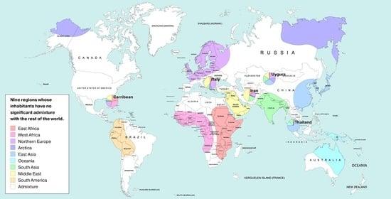
| IDs | Unique Genetic Regions | 3 Reference Populations |
|---|---|---|
| AFE | East Africa | Luhya Webuye Kenya (LWK); Dinka (Sudan); Masai (Kenya) |
| AFW | West Africa | Yoruba (YRI); Esan Nigeria (ESN); Mende Sierra Leone (MSL) |
| AMR | America | Piapoco (Columbia); Wichi (Argentina); Karitiana (Brazil) |
| ARC | Arctica (N Eurasia + N. America) | Koryaks (Russia); Eskimo Sireniki (Russia); Chukchi (Russia) |
| EAS | East Asia | Han China South (CHS); Japanese Tokyo (JPT); Miao (China) |
| EUR | North Europe | Swedes (Sweden); Estonians (Estonia); Germans (Germany) |
| SAS | Hindustan Peninsula | Sri Lankans from UK (STU); Gujarati from Texas (GIH); Mala (India) |
| OCE | Oceania + Australia | Australians (Australia); Papuan (Papua New Guinea); Agta (Philippines) |
| MDE | Middle East | Arabs (Israel); Saudi-Arabians; Palestinian (Israel Central) |
| AFR | AMR | ARC | CAS | CAU | EAS | EUR | MDE | OCE | SAS | SIB | NEA | ANC | |
|---|---|---|---|---|---|---|---|---|---|---|---|---|---|
| AFR | 157 | 128 | 100 | 52 | 96 | 29 | 117 | 108 | 17 | 47 | 54 | 22 | 200 |
| AMR | 128 | 635 | 408 | 322 | 415 | 330 | 435 | 315 | 52 | 316 | 334 | 80 | N/A |
| ARC | 100 | 408 | 1253 | 536 | 475 | 398 | 609 | 409 | 180 | 384 | 683 | 60 | 531 |
| CAS | 52 | 322 | 536 | 641 | 492 | 504 | 522 | 422 | 288 | 457 | 668 | 62 | 412 |
| CAU | 96 | 415 | 475 | 492 | 704 | 428 | 491 | 469 | 44 | 404 | 518 | 57 | 487 |
| EAS | 29 | 330 | 398 | 504 | 428 | 558 | 395 | 354 | 39 | 392 | 466 | 63 | N/A |
| EUR | 117 | 435 | 609 | 522 | 491 | 395 | 670 | 443 | 61 | 453 | 580 | 58 | 585 |
| MDE | 108 | 315 | 409 | 422 | 469 | 354 | 443 | 473 | 25 | 372 | 407 | 57 | 465 |
| OCE | 17 | 52 | 180 | 288 | 44 | 39 | 61 | 25 | 482 | 54 | 254 | 77 | N/A |
| SAS | 47 | 316 | 384 | 457 | 404 | 392 | 453 | 372 | 54 | 478 | 440 | 63 | 403 |
| SIB | 54 | 334 | 683 | 668 | 518 | 466 | 580 | 407 | 254 | 440 | 996 | 62 | 692 |
| NEA | 22 | 80 | 60 | 62 | 57 | 63 | 58 | 57 | 77 | 63 | 62 | N/A | N/A |
| ANC | 200 | N/A | 531 | 412 | 487 | N/A | 585 | 465 | N/A | 403 | 692 | N/A | N/A |
| AFR | AMR | ARC | CAS | CAU | EAS | EUR | MDE | OCE | SAS | SIB | NEA | ANC | |
|---|---|---|---|---|---|---|---|---|---|---|---|---|---|
| AFR | 13.5 | 16.6 | 21.2 | 40.7 | 22.1 | 73.1 | 18.1 | 19.6 | 124 | 45.1 | 39.2 | 192 | 21.2 |
| AMR | 16.6 | 3.3 | 5.2 | 6.6 | 5.1 | 6.4 | 4.9 | 6.7 | 40.7 | 6.7 | 6.3 | 53.0 | N/A |
| ARC | 21.2 | 5.2 | 1.7 | 4.0 | 4.5 | 5.3 | 3.5 | 5.2 | 11.8 | 5.5 | 3.1 | 70.6 | 8.0 |
| CAS | 40.7 | 6.6 | 4.0 | 3.3 | 4.3 | 4.2 | 4.1 | 5.0 | 7.4 | 4.6 | 3.2 | 68.3 | 10.3 |
| CAU | 22.1 | 5.1 | 4.5 | 4.3 | 3.0 | 5.0 | 4.3 | 4.5 | 48.2 | 5.2 | 4.1 | 74.3 | 8.7 |
| EAS | 73.1 | 6.4 | 5.3 | 4.2 | 5.0 | 3.8 | 5.4 | 6.0 | 54.3 | 5.4 | 4.5 | 67.3 | N/A |
| EUR | 18.1 | 4.9 | 3.5 | 4.1 | 4.3 | 5.4 | 3.2 | 4.8 | 34.7 | 4.7 | 3.7 | 73.1 | 7.2 |
| MDE | 19.6 | 6.7 | 5.2 | 5.0 | 4.5 | 6.0 | 4.8 | 4.5 | 84.7 | 5.7 | 5.2 | 74.3 | 9.1 |
| OCE | 124 | 40.7 | 11.8 | 7.4 | 48.2 | 54.3 | 34.7 | 84.7 | 4.4 | 39.2 | 8.3 | 55.0 | N/A |
| SAS | 45.1 | 6.7 | 5.5 | 4.6 | 5.2 | 5.4 | 4.7 | 5.7 | 39.2 | 4.4 | 4.8 | 67.3 | 10.5 |
| SIB | 39.2 | 6.3 | 3.1 | 3.2 | 4.1 | 4.5 | 3.7 | 5.2 | 8.3 | 4.8 | 2.1 | 68.3 | 6.1 |
| NEA | 192 | 53.0 | 70.6 | 68.3 | 74.3 | 67.3 | 73.1 | 74.3 | 55.0 | 67.3 | 68.3 | N/A | N/A |
| ANC | 21.2 | N/A | 8.0 | 10.3 | 8.7 | N/A | 7.2 | 9.1 | N/A | 10.5 | 6.1 | N/A | N/A |
| Sample | Species | Site/Region | Dating (YA) | Coverage | Reference |
|---|---|---|---|---|---|
| Altai, Denisova5 | H. neanderthalensis | Denisova Cave, Altai mountains | 52,000 (122,000) * | 50 | [53] |
| Chagyrskaya 8 | H. neanderthalensis | Chagyrskaya Cave Altai mountains | 60,000 (80,000) * | 27 | [54] |
| Vindija 33.19 | H. neanderthalensis | Vindija Cave, northern Croatia | 45,000 (52,000) * | 30 | [55] |
| Ustishim | H. sapiens | Settlement of Ust’-Ishim in western Siberia | 45,000 | 40 | [56] |
| Denisova | H. denisova | Denisova Cave, Altai mountains | 40,000 (72,000) * | 30 | [18] |
| Stuttgart | H. sapiens | Germany | 7000 | 19 | [24] |
| Loschbour | H. sapiens | Loschbour rock shelter, Luxembourg | 8000 | 22 | [24] |
Publisher’s Note: MDPI stays neutral with regard to jurisdictional claims in published maps and institutional affiliations. |
© 2020 by the authors. Licensee MDPI, Basel, Switzerland. This article is an open access article distributed under the terms and conditions of the Creative Commons Attribution (CC BY) license (http://creativecommons.org/licenses/by/4.0/).
Share and Cite
Khvorykh, G.V.; Mulyar, O.A.; Fedorova, L.; Khrunin, A.V.; Limborska, S.A.; Fedorov, A. Global Picture of Genetic Relatedness and the Evolution of Humankind. Biology 2020, 9, 392. https://doi.org/10.3390/biology9110392
Khvorykh GV, Mulyar OA, Fedorova L, Khrunin AV, Limborska SA, Fedorov A. Global Picture of Genetic Relatedness and the Evolution of Humankind. Biology. 2020; 9(11):392. https://doi.org/10.3390/biology9110392
Chicago/Turabian StyleKhvorykh, Gennady V., Oleh A. Mulyar, Larisa Fedorova, Andrey V. Khrunin, Svetlana A. Limborska, and Alexei Fedorov. 2020. "Global Picture of Genetic Relatedness and the Evolution of Humankind" Biology 9, no. 11: 392. https://doi.org/10.3390/biology9110392
APA StyleKhvorykh, G. V., Mulyar, O. A., Fedorova, L., Khrunin, A. V., Limborska, S. A., & Fedorov, A. (2020). Global Picture of Genetic Relatedness and the Evolution of Humankind. Biology, 9(11), 392. https://doi.org/10.3390/biology9110392