Mass Transport with Asymmetric Peristaltic Propulsion Coated with Synovial Fluid

Abstract

This article aims to model two-dimensional, incompressible asymmetric peristaltic propulsion coated with Synovial fluid (“non-Newtonian model”) with mass transport. Due to the coating of the same base-fluid at the surface of the channel, the boundaries become non-porous and exert no slip on the fluid particles. Two illustrative models for the viscosity, namely, shear-thinning (Model 1) and shear-thickening (Model 2), are considered, which reveal the presence and integrity of coating. The perturbation method has been applied to linearize the complicated differential equations. Model 1 predicted higher viscosity values and more significant non-Newtonian behavior than Model 2. It is also observed that the shear-thinning model behaved in quite the opposite manner for the shear thickening model. The converse behavior of Models 1 and 2 occurs due to a curvature of the flow domain. Moreover, Model 1 is not able to capture the correct exponential viscosity dependence on concentration for the whole range of shear rates. On the other hand, the second model shows a strong relationship with accurate power. Solutions are attained for velocity field, concentration profile, and pressure gradient. The novelty of all the essential parameters is analyzed through graphical results. Furthermore, streamlines are also drawn to determine the trapping mechanism. The present analysis is beneficial in the study of intrauterine fluid dynamics; furthermore, it is applicable in vivo diagnostic; drug delivery; food diagnostics; protein chips; and cell chips and packaging, i.e., smart sensors.

1. Introduction

Synovial fluid is secreted to the cavity by its inner membrane called Synovial [1]. It is a biological fluid filling the Synovial joint-cavity’s several-micrometers-thick layer between the interstitial cartilages [2]. The main component of Synovial fluid is ultrafiltration of the blood plasma devoid of high-molecular proteins, blood cells, and aggressors. Synovial fluid supports joints via high effective cartilage lubrication, while its essential component is an added lubricant called hyaluronan/hyaluronic acid [3]. Several studies showed that the viscoelastic features of Synovial fluid occur due to hyaluronic acid [4]. Hyaluronic acid is natively present in the Synovial fluid in relatively high concentrations [5]. It is experimentally [6] confirmed that the viscoelastic features of Synovial fluids strongly rely on a concentration of hyaluronic acid; therefore, the magnitude of polymerization is substantial, because the volume of hyaluronic random coils exhibits a momentous role in the viscoelastic attributes of Synovial fluid [7,8].

Furthermore, Synovial fluid contains mixtures that reveal a viscoelastic fashion. When a Synovial fluid is propagating with versatile conditions where there is no instantaneous input, then it performs as a Stokesian fluid. When it is only subject to immediate input, then its viscoelastic charactersitics manifests itself. Hron et al. [9] examined the flow analysis of three separate models that could be referred to as Synovial fluid models. These models fit into the type of generalized viscous fluids, whereas only one goes fits into the class of a shear-thinning model in which the power-law exponent relies upon the concentration.

Moreover, incompressible non-Newtonian liquids have attracted great interest in recent years. Perhaps this is due to academic curiosity and their several industrial applications including synthetic lubricants, colloidal fluids, and liquid crystals. It is found that various physiological fluids reveal non-Newtonian behavior. Non-Newtonian characteristics produce satisfactory results when analyzing the mechanism of peristalsis propagating in lymphatic vessels, blood vessels, ductus afferents, intestines, the motion of urine in the human body, food bolus moving through esophagus, the movement of spermatozoa in a vas deferens, the blending of food material, Chyme motion, cilia propagation, blood circulation, and the propagation of bile in a bile duct. A peristaltic movement is a fluid transport that happens because of the contraction and extension of smooth walls. Recently, many authors have determined the peristaltic mechanism in various boundary and initial conditions. Notably, Mekheimer et al. [10] calculated the peristaltic phenomenon of magnetized couple-stress fluid along with the effects of the induced magnetic field. He further achieved the exact analytics solutions for the velocity profile. Srinivas and Kothandapani [11] examined the mass and heat transfer impact on the peristaltic transportation of viscous liquid. They formulated the governing flow using the lubrication approach and obtained the exact solution. Further, they assumed that fluid is travelling in a porous medium having compliant walls. Riaz et al. [12] modeled the unsteady peristaltic flow of Carreau fluid propagating through a small intestine and presented analytic solutions using the perturbation method. Akram et al. [13] explored the behavior of lateral walls on the non-uniform, peristaltic-propelled three-dimensional flow of the couple stress fluid model. Ellahi et al. [14] also discussed the three-dimensional motion of Carreau fluid with an external uniform magnetic field. They used the Homotopy perturbation scheme to obtain the solutions of the obtained non-linear partial differential equations. They determined that the magnetic field is a significant factor in the preservation of the flow field. Bhatti et al. [15] examined the behavior of the oblique magnetic field with heat transfer on the uniform peristaltic motion containing small particles. They presented the exact solutions for the fluid and particulate phases, whereas numerical integration was used to determine the pumping characteristics. Sinha et al. [16] presented the peristaltic motion of viscous liquid containing a variable viscosity under the inclusion of heat exchange and the static magnetic field with asymmetric geometry. They obtained the perturbation solutions under the slip conditions and temperature jump. Shit et al. [17] examined the asymmetrical motion of a micropolar fluid with the induced magnetic field. They obtained exact results for micro-rotation components, magnetic force function, the velocity profile, and the current density profile. A mathematical analysis of a micropolar fluid in an artery having composite stenosis was measured by Ellahi et al. [18]. Bhatti et al. [19] evaluated the peristaltic propulsion of magnetized solid particles in Biorheological fluids. They considered the model of Casson fluid and obtained the exact results for liquid and particulate phase against velocity and temperature profile. Peristaltic motion through a porous channel was presented by Maiti and Misra [20]. They discussed the bile flow with in ducts in the pathological state. Bhatti et al. [21] considered the combined electric and magnetic field impact on the propulsion of the peristaltic third-grade fluid model containing small particles. They further considered the heat transfer effects and obtained the analytical results using Homotopy perturbation methods.

Furthermore, Kabov et al. [22] experimentally discussed the two-phase flow propagating through a microchannel. Mekheimer and Elmaboud [23] addressed the impression of heat exchange and magnetic field on the viscous-fluid model stimulated in peristaltic fashion. They explained the influence of endoscope and bioheat transfer. Elmaboud and Mekheimer [24] addressed the nonlinear peristaltic motion of second-grade fluid propagating through a porous geometry. They further applied the perturbation method to solve the velocity equations, whereas pumping features and friction forces were evaluated by numerical integration. Khan et al. [25] studied the behavior of changeable viscosity of the Jeffrey fluid model propagating through the asymmetric porous channel. Transient peristaltic flow through a permeable finite channel was determined by Tripathi [26]. Chaube et al. [27] discussed the peristaltic flow of the power-law model using the creeping flow regime. Shit et al. [28] also discussed the role of velocity slip on the wavy motion of the couple stress fluid model. They mainly focused on a peristaltic movement in the digestive system. Later, Shit et al. [29] governed the peristaltic biofluid flow through a microchannel. Moreover, they also considered the EMHD (“Electro-Magnetohydrodynamic”) and velocity slip due to a hydrophobic/hydrophilic collision between negatively charged walls. Recently, Zeeshan et al. [30] addressed the behavior of the Sisko fluid model propagating across a non-uniform peristaltic channel. They obtained the second order solution using the Homotopy perturbation method. Some more useful studies related to the topic can be seen in [31,32].

According to literature surveyed, it is observed that no results have been presented yet to examine the behavior of Synovial fluid on peristaltic propulsion through an asymmetric channel. According to our knowledge, not a single mathematical model is given in the literature describing the behavior of Synovial fluid for peristaltic flow. The governing fluid holds the properties of incompressibility and irrotational and constant density. Furthermore, mass transport is also taken into account to discuss the present flow. Mass transportation is also an important phenomenon in the propagation of mass from one region to another region. Therefore, the primary theme of the current study is to present a theoretical and mathematical analysis of the said topic to fill this gap in the literature. The graphical results are presented for two different models of Synovial fluid.

2. Mathematical Modeling

The peristaltic (or “sinusoidal”) motion of Synovial fluid described by generalized incompressible fluid possesses the Navier-Stokes equations with a viscosity depending on a shear rate and concentration. We must couple this system with one extra convection-diffusion equation for a concentration of hyaluronic acid. The fundamental equations of governing flow with synovial fluid model are described in reference [8] as follows:

$$\mathrm{div}V=0$$

(1)

$$\frac{\partial V}{\partial t}+V\cdot \nabla V+\frac{\nabla p}{\mathsf{\rho }}=\frac{2}{\mathsf{\rho }}\mathrm{div}(\mathsf{\Theta })$$

(2)

$$\frac{\partial C}{\partial t}=\mathrm{div}(F(C))-\mathrm{V}\cdot \nabla C$$

(3)

in above equation:

$$F(C)=D_{\mathrm{C}}\nabla C, \mathsf{\Theta }=\mathsf{\mu }(C, D) D$$

(4)

in which ΔV(U,V) is velocity, μ is viscosity, D is symmetric part of velocity gradient, P is pressure, ρ is density, F is concentration flux, C is concentration of hyaluronan/hyaluronic, and D_C is constant diffusivity.

Let us focus on two-dimensional peristaltic flows in an asymmetric channel containing width d₁ + d₂ due to wave traveling in direction of flow with constant velocity c. The flow is discussed in Cartesian coordinates. The mass concentrations upon the upper wall are C₀, whereas on the bottom wall they are C₁. Peristaltic motion on the upper and lower internal surfaces is recognized as

$$H_1(X, t)=Y=d_1+b_1\cos 2\mathsf{\pi }(X-ct)\frac{1}{\mathsf{\lambda }}$$

(5)

$$H_2(X,t)=Y=-d_2-b_2\cos [(X-ct)2\mathsf{\pi }+\mathsf{\lambda }\varphi ]\frac{1}{\mathsf{\lambda }}$$

(6)

To translate the coordinates, we use the same procedure that was used in [13].

The consequent relations of the boundaries of channel are described as

$$h_1(x)=y-1=\mathrm{acos}2\mathsf{\pi }x$$

(7)

$$h_2(x)=y=-b\cos (\varphi +2\mathsf{\pi }x)-d$$

(8)

Synovial Fluid Model

The peristaltic motion of viscous synovial fluid (see [33,34]) with thin film coating at the walls is considered in a two-dimensional channel. The flow patterns corresponding to Models 1 and 2 are markedly different. We shall ignore the detailed discussion here. However, fewer essential points associated with the model are presented. The models under consideration present exciting features. Model 1 is a simple generalized form of a power-law mathematical model for a shear-dependent viscosity that is helpful to define various non-Newtonian fluids in biological and polymer fluid mechanics, food rheology, and geology, to consider the basis of viscosity that affects the concentration of a reactant. Model 2 describes that exponent is a function of concentration.

Model 1: The generalized power-law model and the viscosity are exponentially dependent on concentration, then the Model 1 is written as:

$$\mathsf{\mu }(C, D)={\mathsf{\mu }}_0{\mathrm{e}}^{\mathsf{\alpha }C}{(1+{\mathsf{\gamma }}^2\left|D^2\right|)}^n$$

(9)

Model 2: In this model, a shear-thinning index depends upon the concentration (i.e., zero concentration):

$$\mathsf{\mu }(C, D)={\mathsf{\mu }}_0{(1+{\mathsf{\gamma }}^2\left|D^2\right|)}^{n(C)}$$

(10)

in which,

$$\left|D\right|=\sqrt{2{(\frac{\partial u}{\partial x})}^2+2{(\frac{\partial u}{\partial y})}^2+{(\frac{\partial v}{\partial x}+\frac{\partial u}{\partial y})}^2}$$

(11)

and

$$n(C)=-\frac{{\mathrm{e}}^{\mathsf{\alpha }C}-1}{2{\mathrm{e}}^{\mathsf{\alpha }C}}$$

(12)

in which n is index of shear-thinning comprising values between −0.5 and 0. It is worth mentioning that results of Newtonian fluid are obtained as a particular case of current fluid when n = 0.

The governing equations are too arduous to be acquiescent to stability analysis. Therefore, it is necessary to simplify the modeled equations. Make sure that the simplification process is congruous for such problems. Henceforth, we shall assume the long wavelength constraint, i.e., $\mathsf{\delta }\ll 1$ and less Reynolds number R_e ≈ O(1). Now, it is suitable to make the observing equations dimensionless by defining the following ratios:

$$\begin{array}{l}\overline{y}=\frac{y}{d_1},\alpha ={\alpha }^{\ast }(C_1-C_0), \mathsf{\sigma }=\frac{C-C_0}{C_1-C_0},\overline{\mathsf{\mu }}=\frac{\mathsf{\mu }}{{\mathsf{\mu }}_0}, \overline{h}=\frac{H}{d_1}, \overline{p}=\frac{d_1^{2}p}{\mathsf{\mu }c\mathsf{\lambda }},\mathsf{\delta }=\frac{d_1}{\mathsf{\lambda }}, a=\frac{b_1}{d_1} ,\\ b=\frac{b_2}{d_1},d=\frac{d_2}{d_1}, \mathrm{We}=\frac{\mathsf{\gamma }c}{d_1}, \left|\overline{D}\right|=\frac{d_1}{c}\left|D\right|,S_{\mathrm{c}}=\frac{\mathsf{\mu }}{{\mathsf{\rho }\mathrm{D}}_{\mathrm{C}}}, \overline{v}=\frac{v}{c\mathsf{\delta }}, \mathrm{Re}=\frac{\mathsf{\rho }{d}_{1}c}{\mathsf{\mu }}, \overline{u}=\frac{u}{c},\overline{x}=\frac{x}{\mathsf{\lambda }}\end{array}$$

(13)

In above expression, S_c denotes Schmidt number, Re stands for Reynolds number, α represents concentration production, and γ is a material parameter.

The resulting non-dimensional governing equations along with Models 1 and 2 after exempting bar symbols in a wave frame will observe the following form:

$$\frac{\partial v}{\partial y}=-\frac{\partial u}{\partial x}$$

(14)

$$\frac{\partial p}{\partial x}=\{\begin{array}{cc}\frac{1}{2}\frac{\partial }{\partial y}[(1+\mathsf{\alpha }\mathsf{\sigma })\left\{1+n{\mathrm{We}}^2{(\frac{\partial u}{\partial y})}^2\right\} \frac{\partial u}{\partial y}]\hfill & (\mathrm{Model} 1)\hfill \\ \frac{{\partial }^{2}u}{\partial y^2}-\frac{\alpha {\mathrm{We}}^2}{2}\frac{\partial }{\partial y}[\mathsf{\sigma }{(\frac{\partial u}{\partial y})}^3]\hfill & (\mathrm{Model} 2)\hfill \end{array}$$

(15)

Concentration equation for Models 1 and 2 is simplified to the following form:

$$\frac{1}{S_{\mathrm{c}}}\frac{{\partial }^2\mathsf{\sigma }}{\partial y^2}=0$$

(16)

The no slip boundary conditions become:

$$u(h_1)=-1 u(h_2)=-1, \mathsf{\sigma }(h_1)=0, \mathsf{\sigma }(h_2)=1$$

(17)

3. Solution Procedure

The analytical solutions of Equations (15)–(17) have been determined by regular perturbation method. To solve the problem under consideration, we presented the flow quantities wherein the velocity, concentration, and pressure interns of small Weissenberg number (We) have the following form:

$$u(x, y)=u_{0, i}+{(\mathrm{We})}^2{u}_{1, i}+{(\mathrm{We})}^4{u}_{2, i}+\dots , i=1, 2.$$

(18)

$$\mathsf{\sigma }={\mathsf{\sigma }}_0+{(\mathrm{We})}^2{\mathsf{\sigma }}_1+{(\mathrm{We})}^4{\mathsf{\sigma }}_2+\dots$$

(19)

$$K={(K)}_{0,i}+{(\mathrm{We})}^2{(K)}_{1,i}+{(\mathrm{We})}^4{(K)}_{2,i}+\dots , i=1,2, \dots$$

(20)

in which $K=\frac{\mathrm{d}p}{\mathrm{d}x}$. After the implementation of above expressions in Equations (15)–(17) and equating the exponents of We, one obtains the following systems of equations along with associated boundary conditions.

3.1. Model 1

• System of Order Zero

$$K_{0, 1}=\frac{1}{2}(\mathsf{\alpha }\frac{\partial {\mathsf{\sigma }}_0}{\partial y}\frac{\partial u_{0, 1}}{\partial y}+(1+{\mathsf{\alpha }\mathsf{\sigma }}_0) \frac{{\partial }^2{u}_{0, 1}}{\partial y^2})$$

(21)

$$\frac{1}{S_c}\frac{{\partial }^2{\mathsf{\sigma }}_0}{\partial y^2}=0$$

(22)

Along with the boundary conditions:

$$u_{0, 1}(h_1)=-1, u_{0, 1}(h_2)=-1, { \mathsf{\sigma }}_0(h_1)=0, { \mathsf{\sigma }}_0(h_2)=1$$

(23)

• System of Order One

$$\begin{array}{cc}{K}_{1, 1}=& \frac{1}{2}(\mathsf{\alpha }\frac{\partial {\mathsf{\sigma }}_0}{\partial y}\frac{\partial u_{1, 1}}{\partial y}+(1+{\mathsf{\alpha }\mathsf{\sigma }}_0) \frac{{\partial }^2{u}_{1, 1}}{\partial y^2})+\frac{n\mathsf{\alpha }}{2}\frac{\partial {\mathsf{\sigma }}_0}{\partial y}{(\frac{\partial u_{0, 1}}{\partial y})}^3\hfill \\ & +\frac{3n}{2}(1+{\mathsf{\alpha }\mathsf{\sigma }}_0) {(\frac{\partial u_{0, 1}}{\partial y})}^2\frac{{\partial }^2{u}_{0, 1}}{\partial y^2}\hfill \end{array}$$

(24)

$$\frac{1}{S_{\mathrm{c}}}\frac{{\partial }^2{\mathsf{\sigma }}_1}{\partial y^2}=0$$

(25)

and the boundary conditions:

$$u_{1, 1}(h_1)=0, u_{1, 1}(h_2)=0, { \mathsf{\sigma }}_1(h_1)=0, { \mathsf{\sigma }}_1(h_2)=0.$$

(26)

Obtaining the solutions of the above sets of equations by making use of mathematical software Mathematica 7.0, we have the following results:

• Zeroth Order Solution

$$u_{0, 1}=\frac{1}{\mathsf{\alpha }(\ln (h_2-h_1)-\mathsf{\alpha }\ln (h_2-h_1) (1+\mathsf{\alpha })}[\begin{array}{c}(2(h_1-h_2) {{\rm K}}_{0, 1}(h_2-y)-\mathsf{\alpha }) \ln (h_2-h_1)\\ -(2(-h_2+h_1) {{\rm K}}_{0, 1}(h_1-y)-\mathsf{\alpha })(\mathsf{\alpha }+1) \ln (h_2-h_1) \\ +2{(h_1-h_2)}^2{{\rm K}}_{0, 1}\ln (h_2+y\mathsf{\alpha }-h_1(1+\mathsf{\alpha }))\end{array}]$$

(27)

$${\mathsf{\sigma }}_0=\frac{1-y+a\cos (2\mathsf{\pi }x)}{1+d+a\cos (2\mathsf{\pi }x)+b\cos (2\mathsf{\pi }x+\mathsf{\phi })}$$

(28)

• First Order Solution

$$\begin{array}{cc}{u}_{1, 1}=& \frac{2(h_2-h_1)}{{\mathsf{\alpha }}^4}(h_1-h_2-h_1\mathsf{\alpha }+y\mathsf{\alpha }) [4h_1^{2}n{K}_{0, 1}^3-8h_1{h}_{2}n{K}_{0, 1}^3+4h_2^{2}n{K}_{0, 1}^3\hfill \\ & -K_{1, 1}{\mathsf{\alpha }}^2]+\frac{4{(h_2-h_1)}^{6}n}{\mathsf{\alpha }{(-h_1+h_2+h_1\mathsf{\alpha }-y\mathsf{\alpha })}^2(\ln [h_1-h_2]-{\ln [(h_1-h_2)(1+\mathsf{\alpha })])}^3}{K}_{0, 1}^3\hfill \\ & +\frac{24{(h_2-h_1)}^{5}n}{{\mathsf{\alpha }}^2(-h_1+h_2+h_1\mathsf{\alpha }-y\mathsf{\alpha }){(\ln [h_1-h_2]-\ln [(h_1-h_2)(1+\mathsf{\alpha })])}^2}{K}_{0, 1}^3\hfill \\ & -\frac{2(h_2-h_1) C_1}{{\mathsf{\alpha }}^4({(1+\mathsf{\alpha })}^2{(\ln [h_1-h_2]-\ln [(h_1-h_2)(\mathsf{\alpha }+1)])}^3(\ln [h_2-h_1]-\ln [(h_2-h_1)(1+\mathsf{\alpha })]))}\times \hfill \\ & K_{0, 1}^3+\frac{1}{{\mathsf{\alpha }}^4({(1+\mathsf{\alpha })}^2{(\ln [h_1-h_2]-\ln [(h_1-h_2)(1+\mathsf{\alpha })])}^3(\ln [h_2-h_1]-\ln [(h_2-h_1)(1+\mathsf{\alpha })]))}\hfill \\ & [2(-h_1+h_2) ((-h_1+h_2)((K_{0, 1}^3{C}_2+K_{1, 1}{C}_3) \ln [h_2-h_1]\hfill \\ & +(K_{0, 1}^3{C}_4+K_{1, 1}{C}_5) {(1+\mathsf{\alpha })}^2\ln [(h_2-h_1)(1+\mathsf{\alpha })]))]\hfill \end{array}$$

(29)

$${\mathsf{\sigma }}_1=0$$

(30)

here,

$$K_{0, 1}=\frac{(1+d+h_2-Q-h_1){\mathsf{\alpha }}^2(\ln [h_2-h_1]-\ln [(h_2-h_1)(1+\mathsf{\alpha })])}{{(-h_2+h_1)}^3(2\mathsf{\alpha }+(\mathsf{\alpha }+2)\ln [h_2-h_1]-(2+\mathsf{\alpha })\ln [(h_2-h_1)(1+\mathsf{\alpha })])}$$

(31)

$$\begin{array}{cc}{K}_{1, 1}=& -((1+d-Q){\mathsf{\alpha }}^2(\ln [h_1-h_2]-\ln [(h_1-h_2)(1+\mathsf{\alpha })]))/\hfill \\ & ({(h_1-h_2)}^2(-2h_1\mathsf{\alpha }+2h_2\mathsf{\alpha }+(h_1+h_2)\mathsf{\alpha }\ln [h_1-h_2]-\hfill \\ & 2(h_1-h_2+h_1\mathsf{\alpha })\ln [-h_1+h_2]-h_1\mathsf{\alpha }\ln [(h_1-h_2)(1+\mathsf{\alpha })]-\hfill \\ & h_2\mathsf{\alpha }\ln [(h_1-h_2)(1+\mathsf{\alpha })]+2h_1\ln [(-h_1+h_2)(1+\mathsf{\alpha })]-\hfill \\ & 2h_2\ln [(-h_1+h_2)(1+\mathsf{\alpha })]+2h_1\mathsf{\alpha }\ln [(-h_1+h_2)(1+\mathsf{\alpha })]))\hfill \end{array}$$

(32)

In above-presented equations, C₁–C₅ are some lengthy calculations that have particular values by considering above-given boundary conditions and are defined in Appendix A.

3.2. Model 2

The same contrast as described for Model 1 along with solutions are summarized as:

• System of Order Zero

$$K_{0, 2}=\frac{{\partial }^2{u}_{0, 2}}{\partial y^2}$$

(33)

System of Order One

$$K_{1, 2}=\frac{{\partial }^2{u}_{1, 2}}{\partial y^2}-\frac{\mathsf{\alpha }}{2}\frac{\partial }{\partial y}({\mathsf{\sigma }}_0{(\frac{\partial u_{0, 2}}{\partial y})}^3)$$

(34)

• Zeroth Order Solution

$$u_{0, 2}=\frac{1}{2}(-2+h_1{h}_2{K}_{0, 2}-h_1{K}_{0, 2}y-h_2{K}_{0, 2}y+K_{0, 2}{y}^2)$$

(35)

• First Order Solution

The solution of above equation is examined directly and is prescribed as:

$$\begin{array}{cc}{u}_{1, 2}=& \frac{1}{160(h_1-h_2)}(h_1-y)(h_2-y)(-80h_2{K}_{1, 2}+9h_1^3{K}_{0, 2}^3\mathsf{\alpha }-h_2^3{K}_{0, 2}^3\mathsf{\alpha }-\hfill \\ & 6h_2^2{K}_{0, 2}^{3}y\mathsf{\alpha }+14h_2{K}_{0, 2}^3{y}^2\mathsf{\alpha }-16K_{0, 2}^3{y}^3\mathsf{\alpha }-h_1^2{K}_{0, 2}^3(h_2+26y)\mathsf{\alpha }+\hfill \\ & h_1(80K_{1, 2}+K_{0, 2}^3(9h_2^2-16h_{2}y+34y^2)\mathsf{\alpha }))\hfill \end{array}$$

(36)

here,

$$K_{0, 2}=-\frac{12(-1-d+h_1-h_2+Q)}{{(h_1-h_2)}^3}$$

(37)

$$\begin{array}{cc}{K}_{1, 2}=& -\frac{1}{5{(h_1-h_2)}^7}12(-5h_1^4(1+d-Q)-5h_2^4(1+d-Q)+h_1^3(20h_2(1+d-Q)\hfill \\ & -27\mathsf{\alpha })+27h_2^3\mathsf{\alpha }+81h_2^2(1+d-Q)\mathsf{\alpha }+81h_2{(1+d-Q)}^2\mathsf{\alpha }+27{(1+d-Q)}^3\hfill \\ & \mathsf{\alpha }+h_1^2(-30h_2^2(1+d-Q)+81h_2\mathsf{\alpha }+81(1+d-Q)\mathsf{\alpha })+h_1(20h_2^3(1+d-Q)\hfill \\ & -81h_2^2\mathsf{\alpha }-162h_2(1+d-Q)\mathsf{\alpha }-81{(1+d-Q)}^2\mathsf{\alpha }))\hfill \end{array}$$

(38)

Pressure rise ∆p over one wavelength in dimensionless format is obtained by

$$\Delta p={\int }_0^{1}K\mathrm{d}x$$

(39)

The integral in Equation (41) is evaluated numerically using software package Mathematica 7.0.

4. Graphical Analysis

This study describes a critical analysis with which to approach two different fluid models that can disclose the properties of Synovial fluid when there is no slip at the boundaries and thin-film coating with non-Newtonian thick fluid (Synovial) is applied the walls. A non-linear coupled system of partial differential equations subject to boundary conditions is solved for shear-thinning and thickening models (Models 1 and 2). The complicated equations are solved by a regular perturbation method. To analyze graphically, Figure 1, Figure 2, Figure 3, Figure 4, Figure 5, Figure 6, Figure 7, Figure 8, Figure 9, Figure 10 and Figure 11 have been sketched to measure the behavior of emerging factors on velocity distribution, pressure gradient profile, pressure rise, and trapping phenomena. 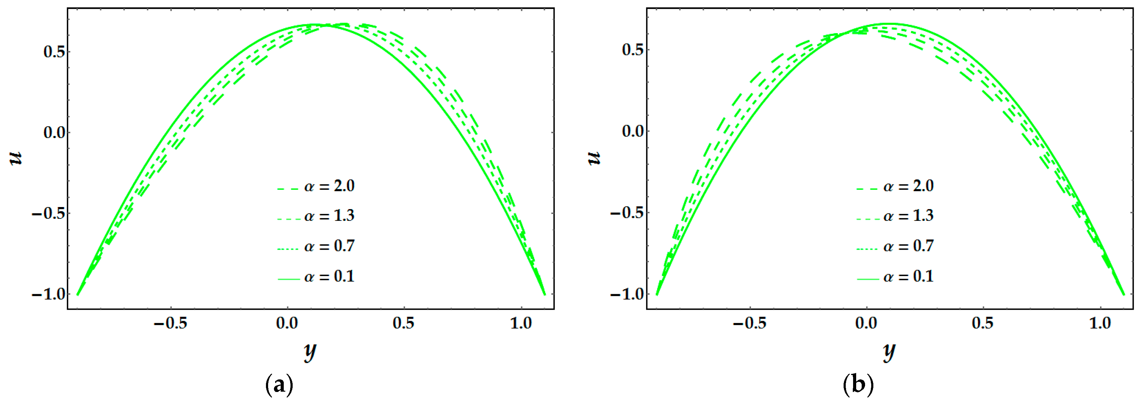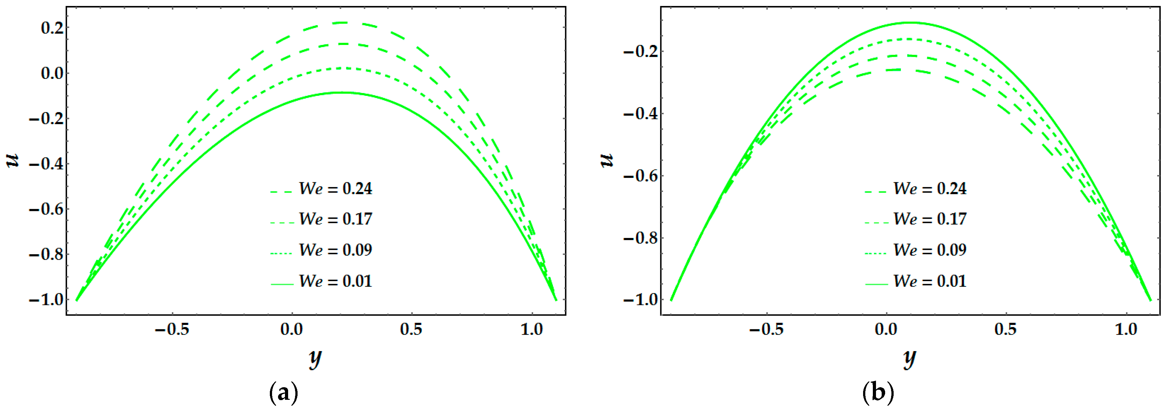Figure 1 and Figure 2 show the effect of concentration parameter α and Weissenberg number We on the velocity component u for both models, respectively. It is extracted that velocity behaves in an opposite manner to shear-thinning and thickening models against multiple values of α. The Weissenberg number is helpful to analyze viscoelastic flows. It is the ratio of elastic forces and viscous forces. In Figure 2, we can understand that the velocity distribution of Model 1 behaves as an increasing quantity for higher values of Weissenberg number. This behavior reveals that elastic forces are dominant over viscous forces. However, the reaction of Model 2 is opposite as matched to Model 1. In Model 2, it can be noticed that viscous forces are dominant over elastic forces. This implies that the nature of shear thinning (Model 1) and the thickening (Model 2) are entirely different. 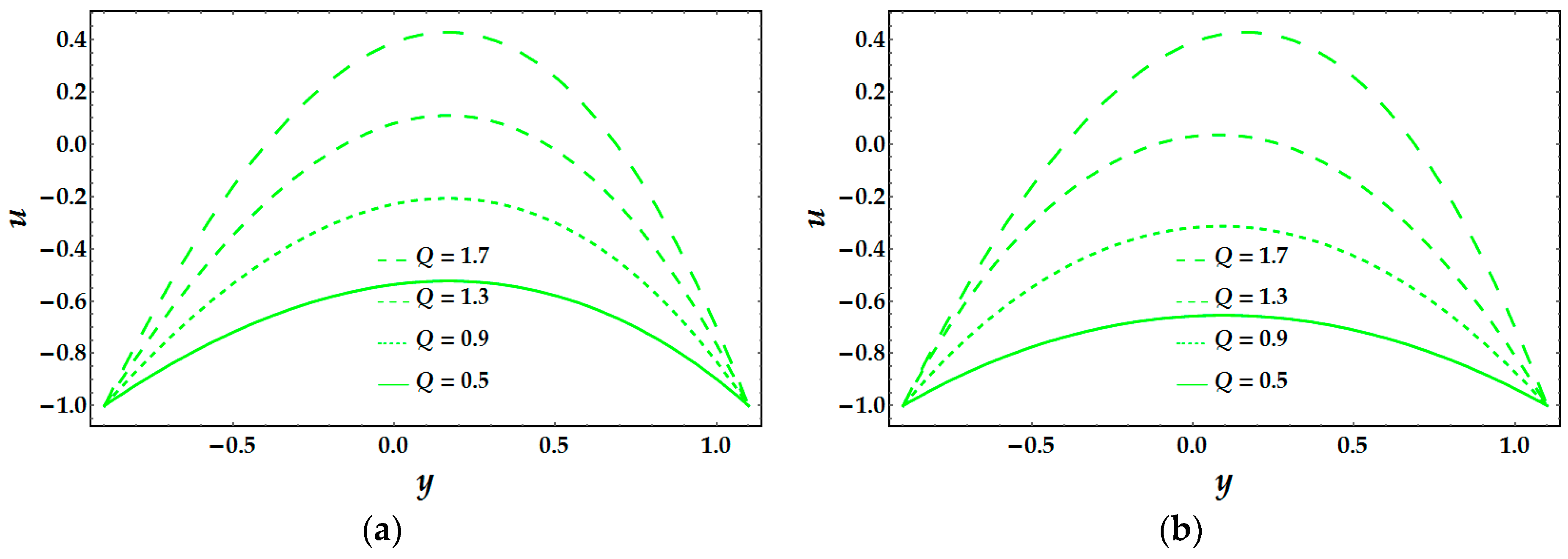Figure 3 displays the dependence of velocity on the average volume flow rate, as expected increase in the value of Q increases the flow velocity in both models.

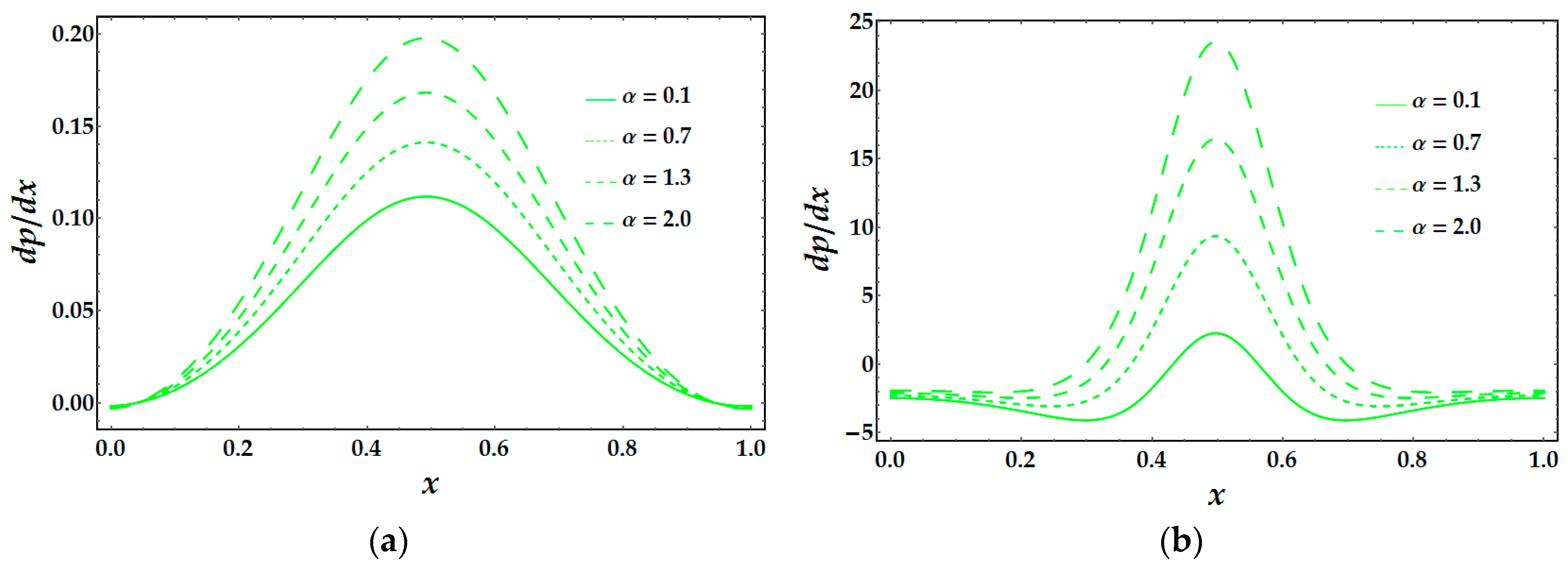
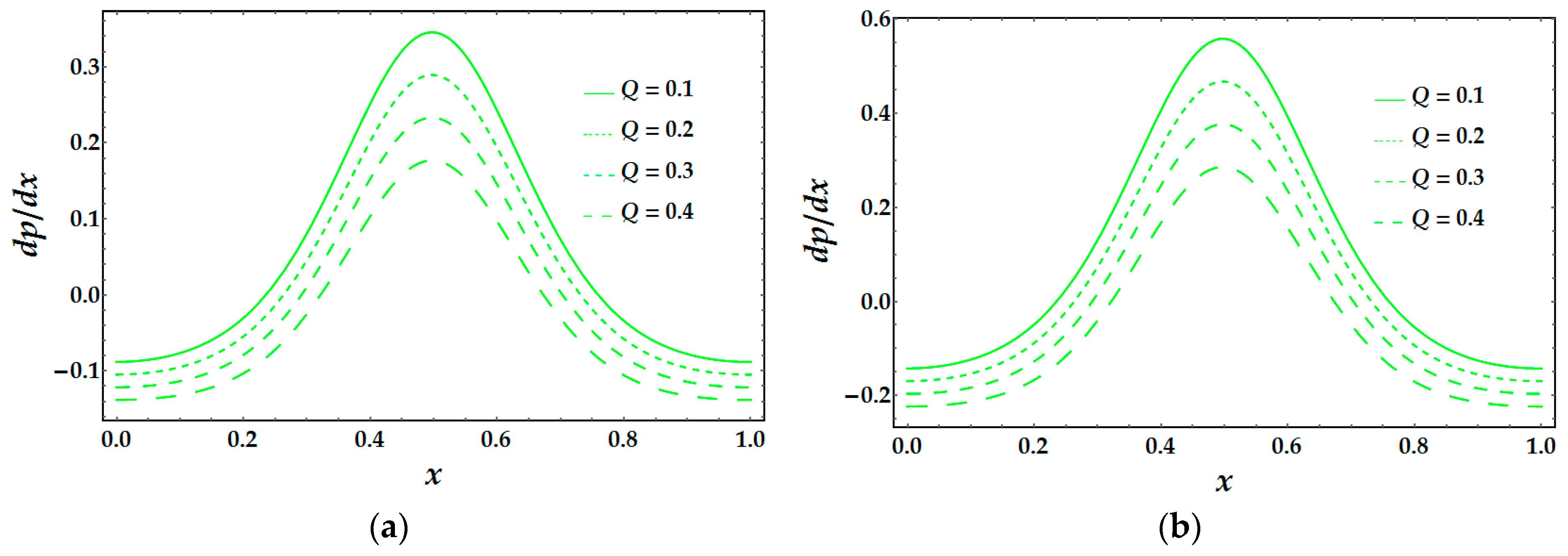
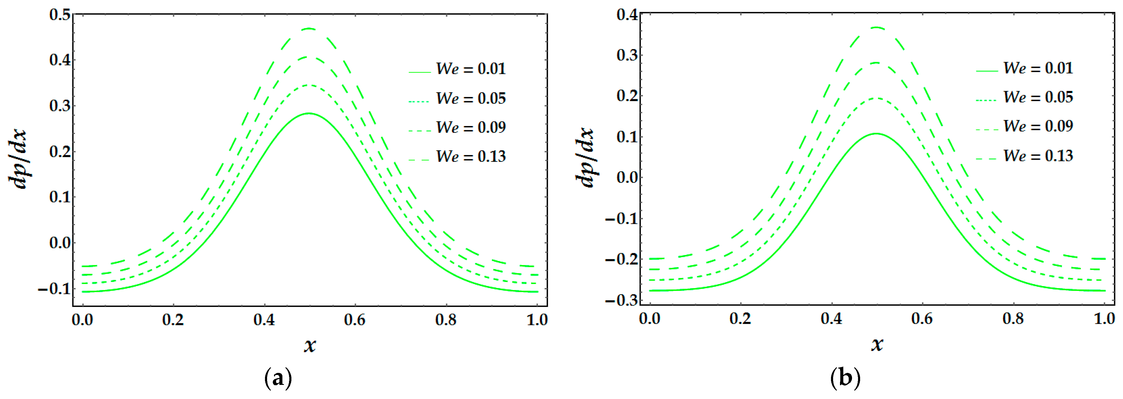
To compare the differences between two models, we include Figure 4, Figure 5 and Figure 6 for pressure gradient dp/dx. In Figure 4 and Figure 5, it is noted that with an excess of α and Q pressure gradient rises. As one can see, the prediction of the viscosity magnitude gets much larger values for the Model 2, unlike Model 1, whereas Weissenberg number We acts in an opposite way, that is, the change in pressure becomes larger throughout the flow and smaller for Model 2 than for Model 1 (see Figure 6).

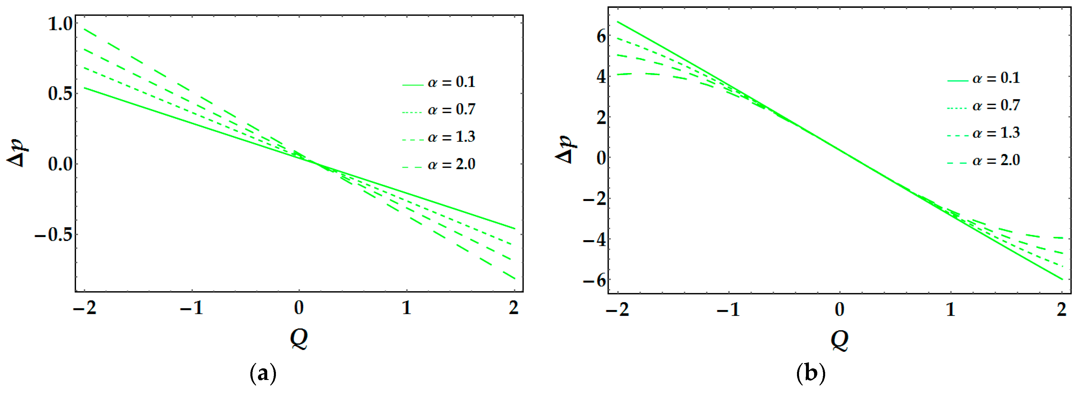
Figure 7, Figure 8 and Figure 9 are plotted to determine the behavior of pumping rate in different regions. The pumping features can be examined by the pressure rise (Δp) versus the average volume flow rate/mean flux Q. The complete area is divided into four quarters [13]. Figure 7a describes the pressure rise Δp under the variety in values of α. It is observed that pressure rise is linearly dependent on flow rate, and free pumping is attained at Q = 0. It is evaluated here that while increasing α, the pressure rise Δp decreases in Region II, whereas it increases in Region III. Figure 7b is plotted for Model 2, and one can easily infer from it that dependence is not linear other than in α = 0.1. 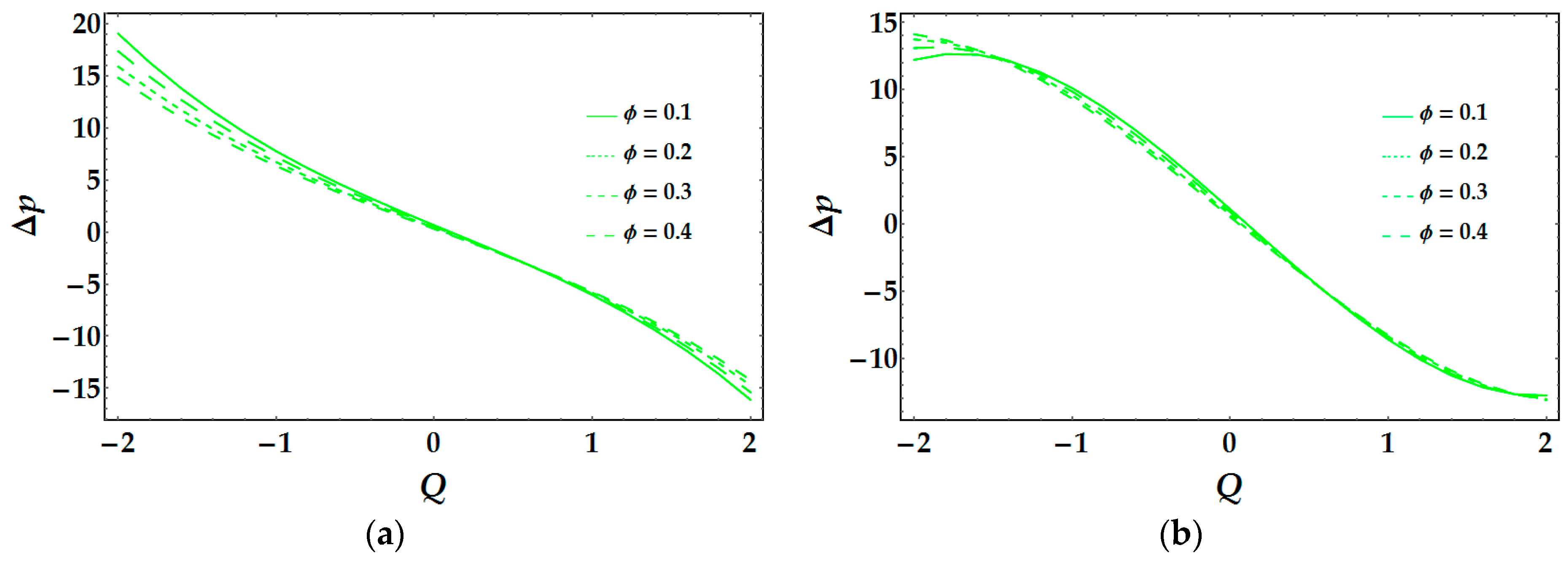This figure indicates that with an increase in α, magnitude of Δp decreases in Region III and has opposite behavior in other two regions. The effects of phase angle φ on Δp are depicted in Figure 8. For Model 1, we can visualize that there is an increase of pressure rise in Region II when φ increases, while the reverse situation is found in Region II and remains consistent in Region I. It is entirely possible that the opposite behavior of Model 1 and Model 2 is due to the curvature in the flow domain. 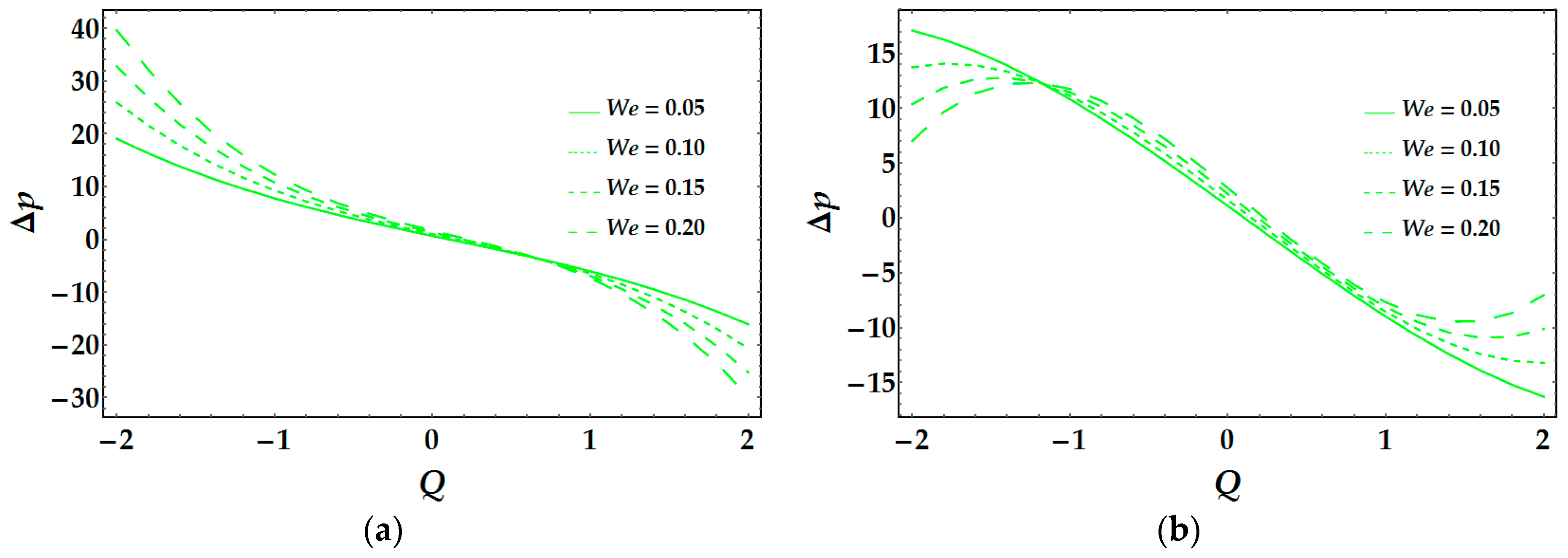Figure 9a examines the influence of Weissenberg number We on Δp for Model 1. It is noticed that Δp increases by increasing We in Regions I and II, while the reduction in pressure rise is seen in Region III. On the other hand, the behavior of pressure gradient for We is also noted in Figure 9b. Model 2 shows a continuous increase in the Region I, hasty fall in Region II, and a drastic increase in Region III.

Trapping scheme is another important mechanism for analyzing flow pattern. However, in peristaltic (or sinusoidal) motion, a closed contour of streamlines can be examined at time-averaged flow rate and different values of amplitude. This phenomenon is known as trapping. According to the physiological point of view, the fluids can be trapped due to continuing movements of smooth boundaries, which are beneficial to adequately propel the working biological liquid from one point to another point. Due to proper prorogation, the working organs can stay alive for a long time without any difficulty. Therefore, the trapping phenomena can be observed by sketching stream functions against the concentration parameter α and the volume flow rate Q. Figure 10 and Figure 11 are drawn to show the trapping phenomena. 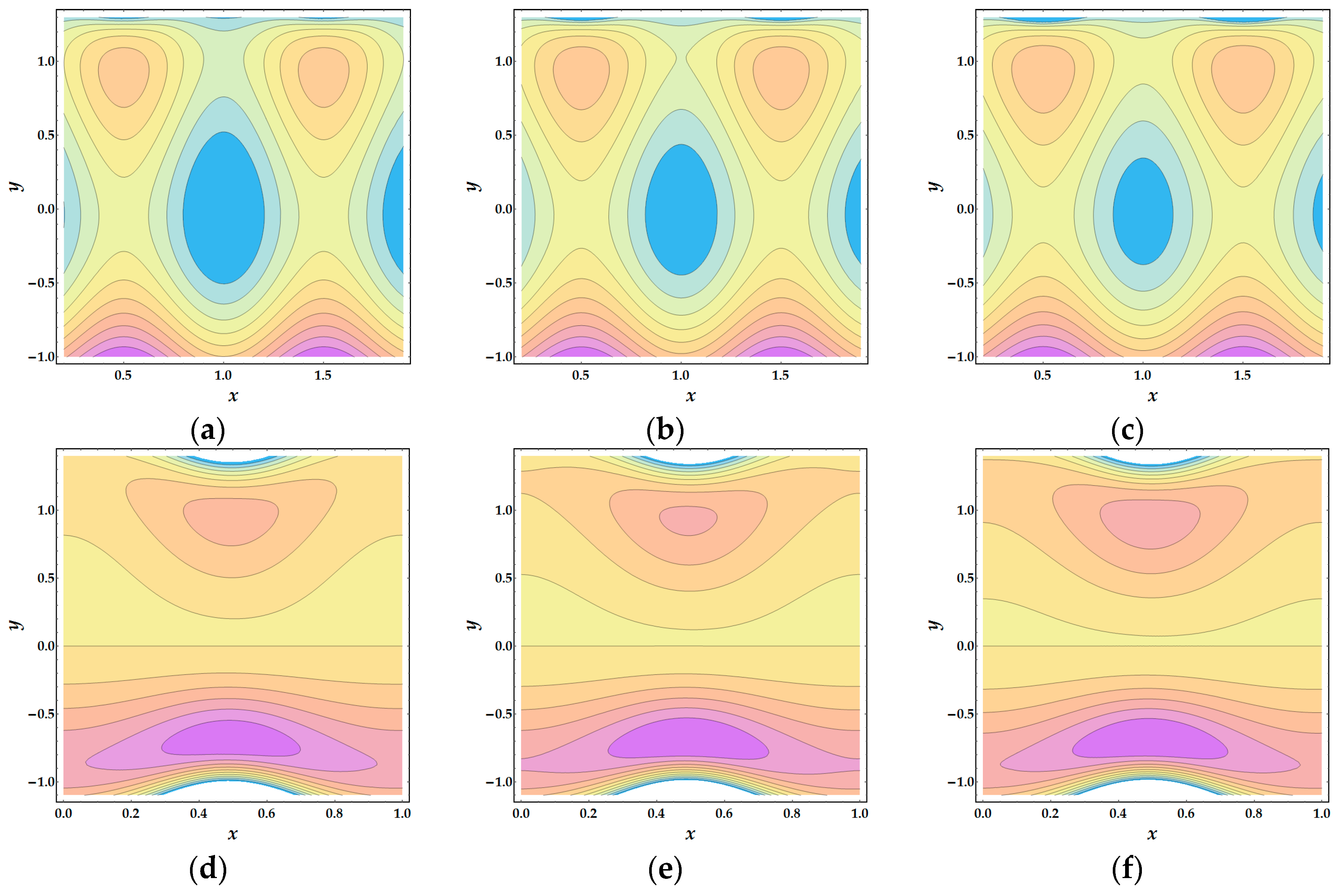Figure 10a–c is illustrated for Model 1. It is observed that for changing values of α, a large bolus is formed at the center that decreases in size and increases in α. For Model 2, Figure 10d–f shows as α increases the bolus formed above y = 0 decreases in size, whereas below y = 0 it increases, and more boluses are obtained with large values of α. 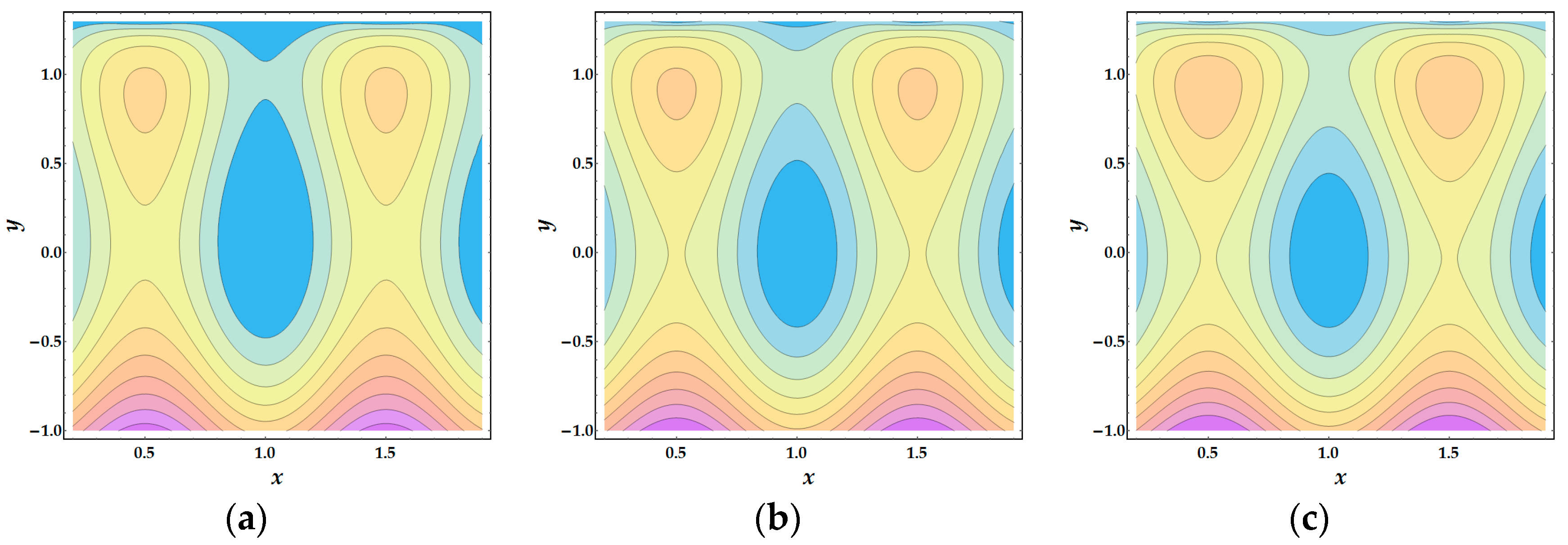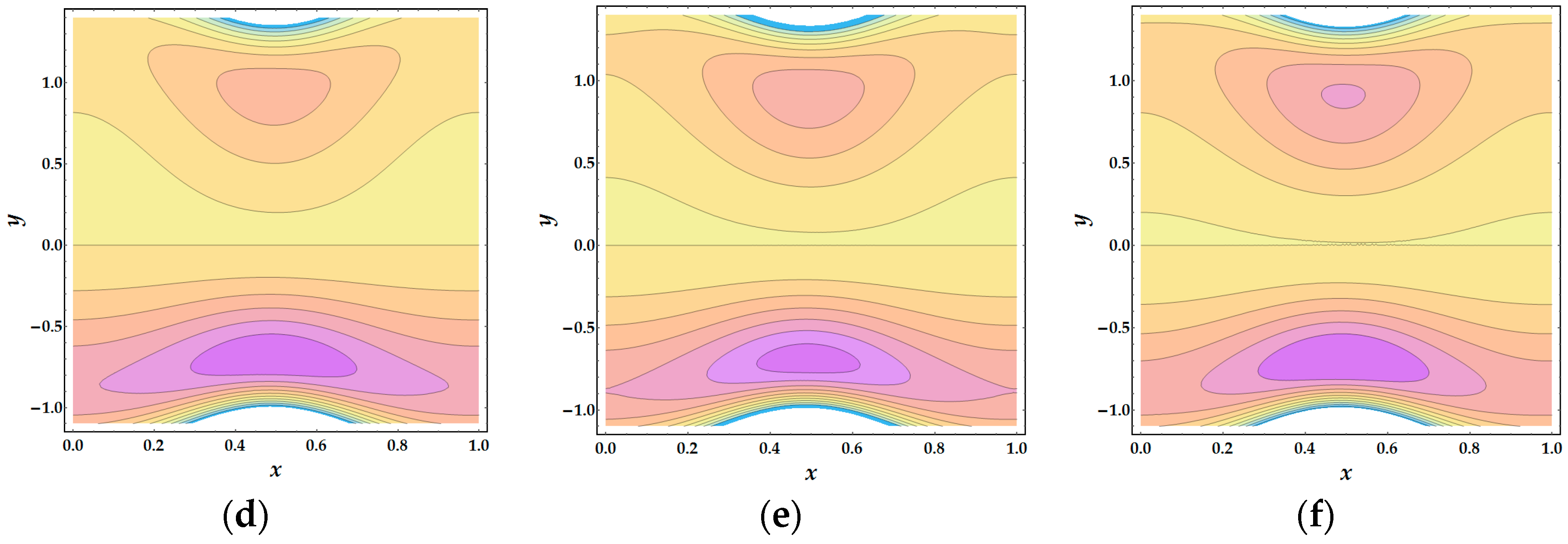Figure 11 shows the effect of variation of Q on trapping. It can be analyzed that with an increase in Q, bolus decreases and increases in size above and below y = 0, respectively. The present investigation is also suggested for three-dimensional flow configuration with appropriate assumptions and modifications.

5. Conclusions

In the current analysis, we examined theoretically the peristaltic motion of Synovial fluid in the two-dimensional asymmetric channel in the presence of coating on the walls exposing thin-film layers. The Synovial fluid has viscoelastic material; it can be described under specific physical conditions such as non-Newtonian fluid. We have considered two models for viscosity to capture shear-thinning properties and viscosity dependence on the concentration of hyaluronic acid. Analytic solutions for velocity, concentration, and pressure gradient are first produced using the regular perturbation method, and then the behavior of pertinent parameters is examined and discussed graphically. The expression of pressure rise is obtained numerically. The contours have also been drawn to explain the action of the trapping bolus phenomenon. The model with the shear-thinning index is directly dependent on the concentration of hyaluronic acid, which seems to be appropriate. According to our knowledge, no studies have been presented before that can describe the concentration effects on shear-thinning and thickening models for the peristaltic flow of Synovial fluid. Solutions are carried out for velocity, concentration field, and pressure gradient. The behavior of all the governing parameters is shown and scrutinized. The present analysis is also applicable for experimental investigation and assurance to give reliance for the significance of the governing nonlinear-boundary value problem.