Article

Simulation of Acoustic Wave Propagation in Aluminium Coatings for Material Characterization

1
Materials Center Leoben Forschung GmbH (MCL), Leoben 8700, Austria
2
Institute of Physics, Karl-Franzens University of Graz (KFU), Graz 8010, Austria
3
PVA TePla Analytical Systems GmbH (PVA AS), 73463 Westhausen, Germany
4
Infineon Technologies Austria AG (IFAT), Villach 9500, Austria
*
Author to whom correspondence should be addressed.
Coatings 2017, 7(12), 230; https://doi.org/10.3390/coatings7120230
Submission received: 28 September 2017 / Revised: 23 October 2017 / Accepted: 4 December 2017 / Published: 14 December 2017
(This article belongs to the Special Issue Modelling and Simulation of Coating)

Abstract

:
Aluminium coatings and their characterization are of great interest in many fields of application, ranging from aircraft industries to microelectronics. Here, we present the simulation of acoustic wave propagation in aluminium coatings via the elastodynamic finite integration technique (EFIT) in comparison to experimental results. The simulations of intensity (I)–defocus (z) curves, obtained by scanning acoustic microscopy (SAM), were first carried out on an aluminium bulk sample, and secondly on a 1 µm aluminium coating deposited on a silicon substrate. The I(z) curves were used to determine the Rayleigh wave velocity of the aluminium bulk sample and the aluminium coating. The results of the simulations with respect to the Rayleigh velocity were corroborated by non-destructive SAM measurements and laser ultrasonic measurements (LUS).

1. Introduction

Aluminium coatings offer a variety of favourable properties, including high reflectivity, high conductivity, high corrosion resistance, and low costs. The benefits of aluminium coatings render them attractive candidates for large-scale applications in aircraft industries, and also for implementation in small-scale devices, concerning micro- and nano-electronics [1].
The frequent use of aluminium coatings increases the demand for their precise characterization. However, some state-of-the-art methods show drawbacks concerning thin film characterization; e.g., they require the direct loading of the sample [2]. Alternatively, ultrasonic waves can be used in order to determine thin film properties; e.g., via laser-induced ultrasound (LUS) [3,4,5,6] or via scanning acoustic microscopy (SAM) [7,8].
SAM represents a well-established tool in state-of-the-art failure and material characterization, providing high potential regarding automation [9], allowing fast and accurate failure detection. With commercially available SAM set-ups, the challenge lies mainly in (1) the necessary specific hardware for the measurement (e.g., emitter/sensor), high time resolution (ps), and accurate movement of emitter/sensor over the sample, and (2) in the interpretation of the SAM data—which can be quite cumbersome due to the presence of various wave modes in thin films.
One outstanding attribute of acoustic microscopy is the possibility to monitor the intensity I of the reflected sound waves as a function of the defocus position z—also called V(z) curves or acoustic material signatures (AMS) [7,8]—from which the Rayleigh wave velocity of the analysed material can be obtained.
The I(z) measurement relies on the excitation of Rayleigh waves that propagate on the sample surface and leak back to the piezoelectric transducer. Decreasing the distance between lens and sample, the Rayleigh contribution interferes with the acoustic field reflected from the sample—alternating destructively and constructively, resulting in an oscillation of the measured intensity I as function of the defocus position z.
The Rayleigh wave velocity can be used directly for material characterization or material monitoring [10,11], or alternatively, material properties can be extracted [3,4,5,6,7,8]. In layered media, the Rayleigh velocity depends on frequency if the analysed coatings are thinner than approximately 1–2 wavelengths [12,13]. Considering a broad-band Rayleigh wave, the lower frequency part of the wave propagates more in the substrate, whereas higher frequency components travel mainly in the coating due to their lower penetration depth. Consequently, the Rayleigh wave velocity becomes dispersive (i.e., depends on frequency); this effect has been extensively studied in the past (e.g., [13,14,15]). The dispersion of the Rayleigh wave can be used to extract elastic mechanical parameters like the Young´s modulus, because the Rayleigh wave velocity depends on the density as well as the elastic constants. In this sense, the determination of the Rayleigh wave velocities is of high interest for the characterization of materials—especially of coatings—and was studied via LUS in, e.g., [3,4,5,6] and via SAM in, e.g., [8,16,17,18,19]. In the past, I(z) measurements have been investigated analytically via ray theory [7,20,21] and via wave theory approaches [7,22].
For general numerical elastic wave propagation, finite element [23,24,25], spectral element [26,27], pseudospectral [28,29], finite volume methods [30], finite difference [31,32,33,34], and the elastodynamic finite integration technique (EFIT) [35,36] can be found in the literature. It is a common feature of all real-space numerical schemes for elastic wave propagation in higher dimensions that the linear dispersion relation of the wave equation is not reproduced exactly, but numerical dispersion errors are introduced. Severe dispersive errors and even spurious solutions force standard finite element methods (FEMs) with low-degree ansatz functions to use excessively high mesh densities [23,24,25]. In this work, to access the I(z) curves we use EFIT for the full elastic wave propagation, because of its good compromise in terms of accuracy relative to its computational cost. The field variables, velocity and stress, are placed in a staggered manner onto the computational grid, which greatly improves the dispersion relation of the scheme. Interestingly, this property is also exploited in electrodynamics, where the finite difference time domain (FDTD) scheme is unsurpassed for inhomogeneous domains [37], and recently also for the relativistic wave equation [38]. The elastic wave discretization using a staggered grid and the EFIT are related, with the difference being that the material properties are placed differently on the grid, allowing the EFIT to more accurately describe material inhomogeneities [35].
We simulated the I(z) curve for an aluminium bulk sample for calibration, because bulk values for aluminium can be found in the literature (e.g., [7]). In addition, the Rayleigh wave velocity can be measured very accurately via LUS [3,4,5,6]. After this calibration step, the I(z) curve of an aluminium-coated silicon sample was simulated and directly compared to results obtained from SAM measurements. The Rayleigh wave velocity—as a material parameter—was obtained from the EFIT simulation and from the SAM measurement, using a 400 MHz acoustic lens. The SAM and the LUS measurements corroborated the EFIT simulation results regarding the Rayleigh wave velocity of the aluminium sample and the aluminium coating. The use of full wave simulation as tested here on aluminium bulk and coated samples allows for arbitrarily varying real thickness and material property distribution up to complex geometrical structures like microelectronics components.
Although ray theory approaches outperform the EFIT simulation of I(z) curves with respect to time-efficiency in general, the EFIT simulation provides more possibilities with respect to: (a) depicting the sound field propagation for various time-steps in the measurement, (b) creating an A-scan equivalent, (c) analysing the influence of, e.g., anti-reflective coating (ARC) or damping of the coupling liquid, and (d) most notably, complex multi-layered structures—relevant for, e.g., micro- and nanoelectronic devices—can be conveniently analysed via state-of-the-art EFIT simulations.

2. Materials and Methods

2.1. Sample

The analysed sample was a 4 × 2 cm2 segment of an aluminium-coated silicon wafer with (100) crystallographic orientation. The aluminium layer was deposited via physical vapour deposition, and its thickness was determined via profilometry. In addition, the density of 2.709 g/cm3 of the aluminium thin film was determined via X-ray diffraction (XRD) using a D8 Discover system (Bruker, Billerica, MA, USA).

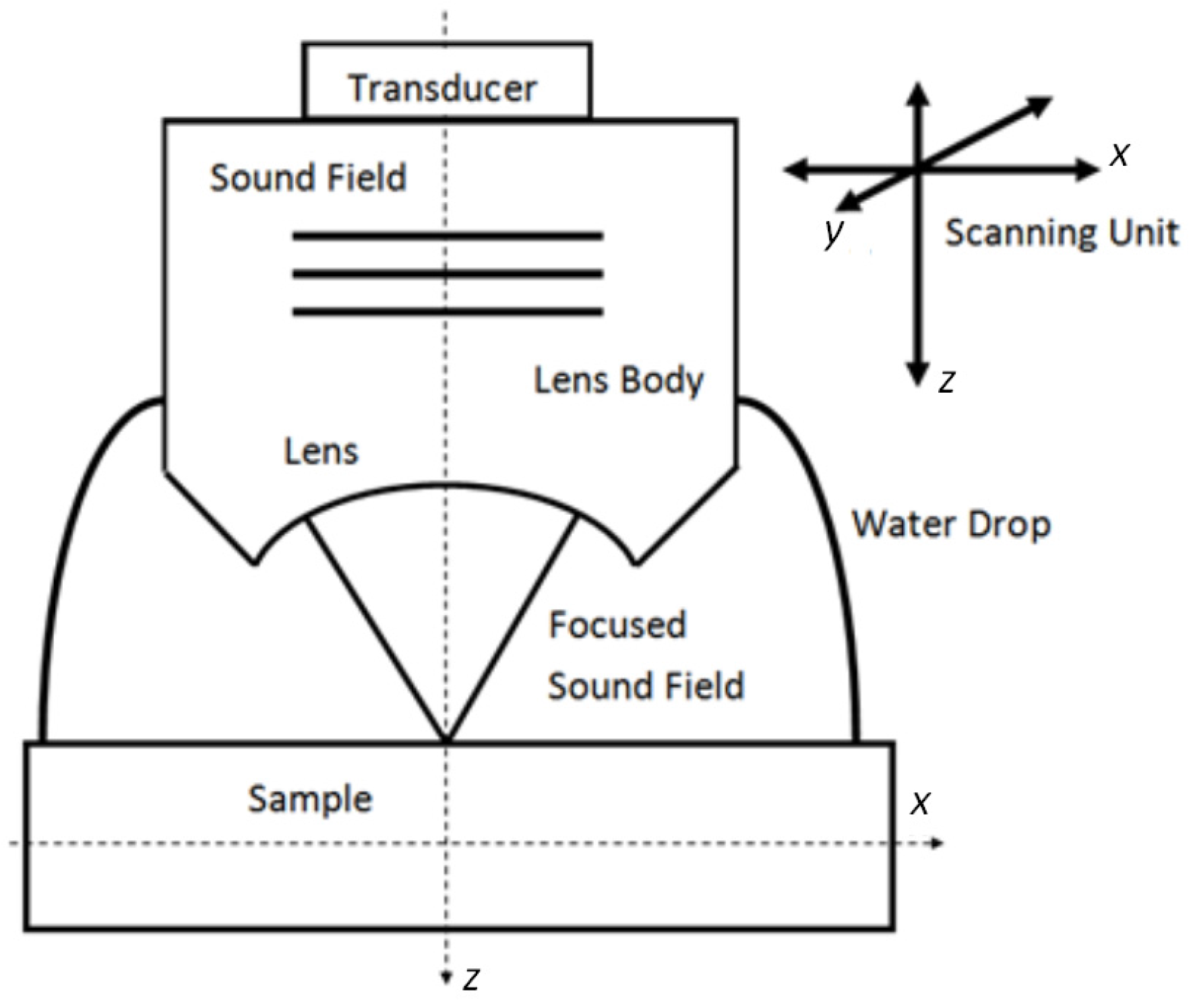
2.2. Scanning Acoustic Microscopy (SAM)

In scanning acoustic microscope measurements, piezoelectric transducers (emitter/sensor) are used to generate ultrasonic waves (see Figure 1), e.g., [7]. The sound waves are focused onto or below the surface of the investigated sample via an acoustic lens. At the sample–water interface, part of the acoustic field is reflected and propagates back to the transducer. At the transducer, the reflected acoustic field is converted into a time-variant electric signal which is presented in time domain and commonly referred to as A-scan (see e.g., [39]).
If the opening angle of the lens exceeds the critical Rayleigh angle θ R ,
θ R = sin 1 ( v 0 v R )
Rayleigh waves can be excited at the surface of the sample (Equation (1)). Here, ν0 denotes the sound velocity in water, which is approximately 1500 m/s at room temperature. Once excited, the Rayleigh wave propagates along the surface and leaks energy back to the lens and subsequently to the transducer. At the piezoelectric element of the transducer, the phase and amplitude of the longitudinal sound wave reflected from the sample and the leaky Rayleigh wave are summed up [7]. The two wave modes (Rayleigh and longitudinal wave) interfere alternating constructively and destructively, depending on the defocus position of the transducer. According to [7], the periodicity ∆z of the oscillation depends on the Rayleigh sound velocity νR of the investigated sample via
z =   λ 0 2   ×   ( 1 cos θ R )  
where λ0 denotes the wavelength of the sound wave in water, see Equation (2).
A SAM can be operated in either pulsed or tone-burst mode [22]. The generally longer excitation time in tone burst mode results in signals which are very narrow in the frequency domain, allowing precise frequency-dependent measurements.
In the work reported here, a commercially available SAM 400 (PVA, Analytical Systems GmbH, Westhausen, Germany) was operated in reflection mode, equipped with a custom-built tone-burst set-up, to perform precise frequency-dependent measurements. For the calibration measurement on bulk aluminium, an acoustic objective (AO) was used with a transducer of 400 MHz nominal centre frequency and an opening angle of 120° (PVA, Analytical Systems GmbH, Westhausen, Germany). The resonance frequency of the transducer was found at approximately 430 MHz. In the case of the aluminium coating, an acoustic objective with an opening angle of 60° was applied (PVA, Analytical Systems GmbH, Westhausen, Germany). Operated in tone-burst mode, the transducer was addressed at approximately 400 MHz, at the resonance frequency of the transducer. The I(z) curve was monitored with a step size of 2 µm in the case of the calibration measurement and in the case of the coating measurement. From the periodicity Δz of the I(z) curves, the Rayleigh wave velocities were extracted.

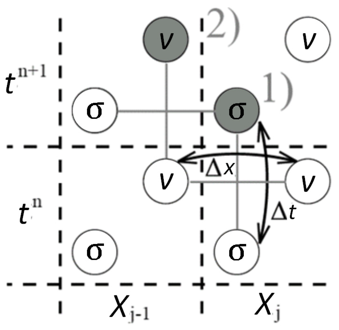
2.3. Elastodynamic Finite Integration Technique (EFIT)

The description of ultrasonic sound field propagation simulation in isotropic linear elastic materials, discretized via the elastodynamic finite integration technique, can be found in [35].
The underlying set of differential equations is given by the kinetics
ρ v t = × σ
the kinematics
d ϵ d t 1 2 [ (   v ) + (   v ) T ]
and the constitutive (or material) law relating them by σ E ·   ϵ
ρ is the mass density, v is the particle velocity field (being the first derivative of the displacement field u with respect to time), ϵ is the (second rank) strain tensor, σ is the (second rank) stress tensor, and E is the (forth rank) stiffness tensor. As shown in Figure 2, the velocities and stress field variables are discretized in a staggered manner on the spatial grid together with a leap-frog updating procedure in time (c.f. Figure 2) [35]. It is shown in [35] that the scheme can be written for arbitrary anisotropy and inhomogeneity of the elastic material behaviour.
Figure 3 shows EFIT results for the SAM measurement of a coated sample at nine time-steps. In accordance with the SAM measurement, an anti-reflective coating (ARC) on the lens was implemented. The ultrasonic field is depicted by the normalized magnitude of the z-component of the velocity field in Figure 3. The sound wave is excited by the transducer in Figure 3, time-steps 1 and 2, and propagates from top to bottom through the lens body (time-step 3) towards the surface of the sample (time-step 4). At the surface (time-step 5), part of the sound field is transmitted into the sample (time-step 6). The remaining sound field is reflected and travels back to the lens at time-steps 7 and 8. At time-step 9, the reflected sound waves reach the transducer. The artificial A-scan is obtained by summing up the z-component of the velocity field along the width of the transducer at the position of the transducer.
The I(z) measurement, carried out via SAM, was simulated for the case of (1) an aluminium block of approximately 40 × 50 × 3 mm3, referred to as bulk aluminium, and (2) an aluminium coating of approximately 1 µm thickness, deposited on a silicon wafer (100). In accordance with the SAM measurement, we implemented a transducer of approximately 430 MHz centre frequency and a lens-opening angle of 120° in the simulation for case (1). For the simulation, isotropic linear elastic material behaviour was assumed, in accordance with [13]. The assumption of isotropy is made for aluminium because its Zener anisotropy ratio is close to one [40]. Literature values for the longitudinal and transversal sound velocity and the density of aluminium were used as input values [7,40]. The simulation was carried out for more than 30 defocus positions, and the A-scan data was assembled for each of them. From the A-scan data, the relevant time window was identified, and the intensity was computed and integrated over the identified time interval. For case (2), the aluminium coating on a silicon substrate, literature values for the longitudinal and transversal sound velocity and the density of aluminium as well as silicon were used as input values, taken from [7,40]. The simulation was carried out for a transducer of 400 MHz centre frequency and a lens-opening angle of 60°. For more than 30 defocus positions, the A-scan data were computed and the intensity of the acoustic signal as a function of the defocus position z was computed. The frequency-dependent damping of the coupling liquid was implemented via an exponential damping factor in the simulation, and due to the spherical focus of the lens used in the SAM measurement, an axial symmetric simulation along the z-axis was performed [36].

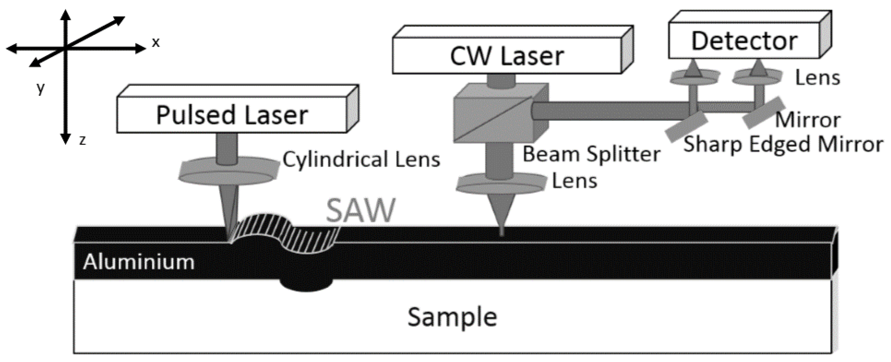
2.4. Laser Ultrasound (LUS)

The laser ultrasonic measurement is described in [3,4,5,6]. Here, a pulsed laser is focused via a cylindrical lens on the sample surface, exciting a Rayleigh wave. A second, continuous wave laser is used in order to detect the Rayleigh wave, using a beam deflection approach. A schematic of the set-up is shown in Figure 4. From the measurement at two detection points, the phase velocity of the Rayleigh wave vR as function of frequency f (Equation 3) can be determined via [3,4,5,6]:
v R ( f ) = ( x 2 x 1 )   2   π f Φ 2 ( f ) Φ 1 ( f )  
In Equation (3), x2x1 is the distance between the detection points and Φ denotes the phases of the Fourier-transformed laser-induced signals.
In the case of (1), the calibration measurement on bulk aluminium, Rayleigh waves were excited via a pulsed laser at 11 positions. The applied Nd:YAG laser has a pulse width of approximately 2 ns, a repetition rate of 10 Hz, and a wavelength of 532 nm. For the 11 cases, the excited Rayleigh waves were detected via a second continuous wave laser. The time at which the Rayleigh waves passed the detection point are plotted as function of the distance the waves travelled in Figure 5.
For the aluminium coating, the pulsed laser from the calibration measurement was used in order to excite broadband Rayleigh waves on the sample. The measurement was performed in the frequency range up to 200 MHz. The Rayleigh wave velocity was obtained from the measurement at two detection points via Equation (3). Since the Rayleigh wave velocity depends on frequency in the case of a coated sample, a theoretical model for the evaluation of the dispersion curve was considered [13]. In the theoretical model, isotropic material behaviour is assumed. This assumption is valid if the measurement is carried out along a symmetry axis of the silicon [3,4,5,6]. Our measurements were performed along the [110] symmetry axis of the silicon sample.

3. Results

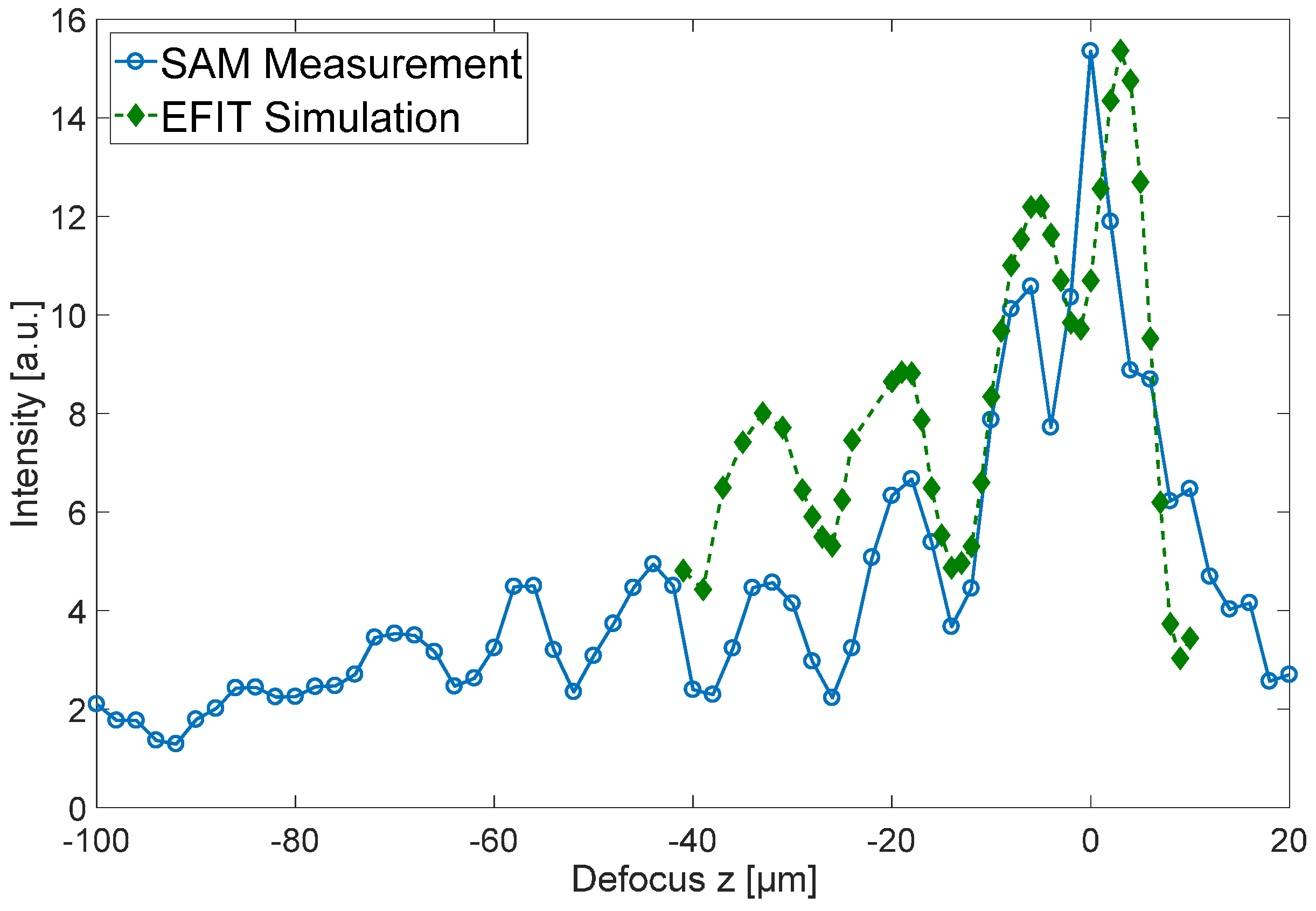
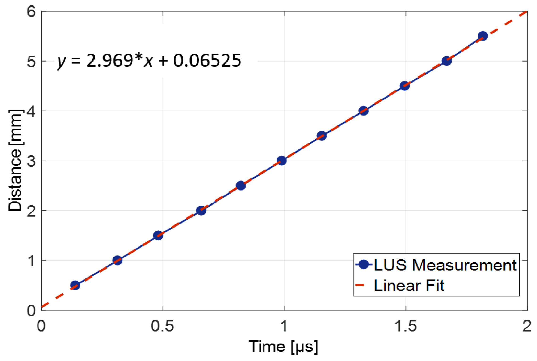
3.1. Aluminium Bulk Sample for Calibration

In the case of the aluminium sample, the simulated intensity I as function of the defocus positions z is shown in Figure 6, in direct comparison to the SAM measurement. From Figure 6, the periodicity of the I(z) oscillation Δz was determined and used to calculate the Rayleigh wave velocity vR via v R f v 0 Δ z , according to [22]. In [22], the important property of the I(z) curves in the evaluation of Rayleigh wave velocities is appointed to be Δz, not the amplitude. However, differences in the amplitudes of the I(z) curves in Figure 6 might stem from actual higher damping coefficients (e.g., for water we used literature values for the damping coefficient; the damping in the sapphire lens body is not included in our simulations). Concerning the LUS measurement, the slope of the linear fit in Figure 5 was used to determine the Rayleigh wave velocity. The EFIT, SAM, and LUS results are listed in Table 1, in comparison to a literature value for the Rayleigh wave velocity in bulk aluminium [7].

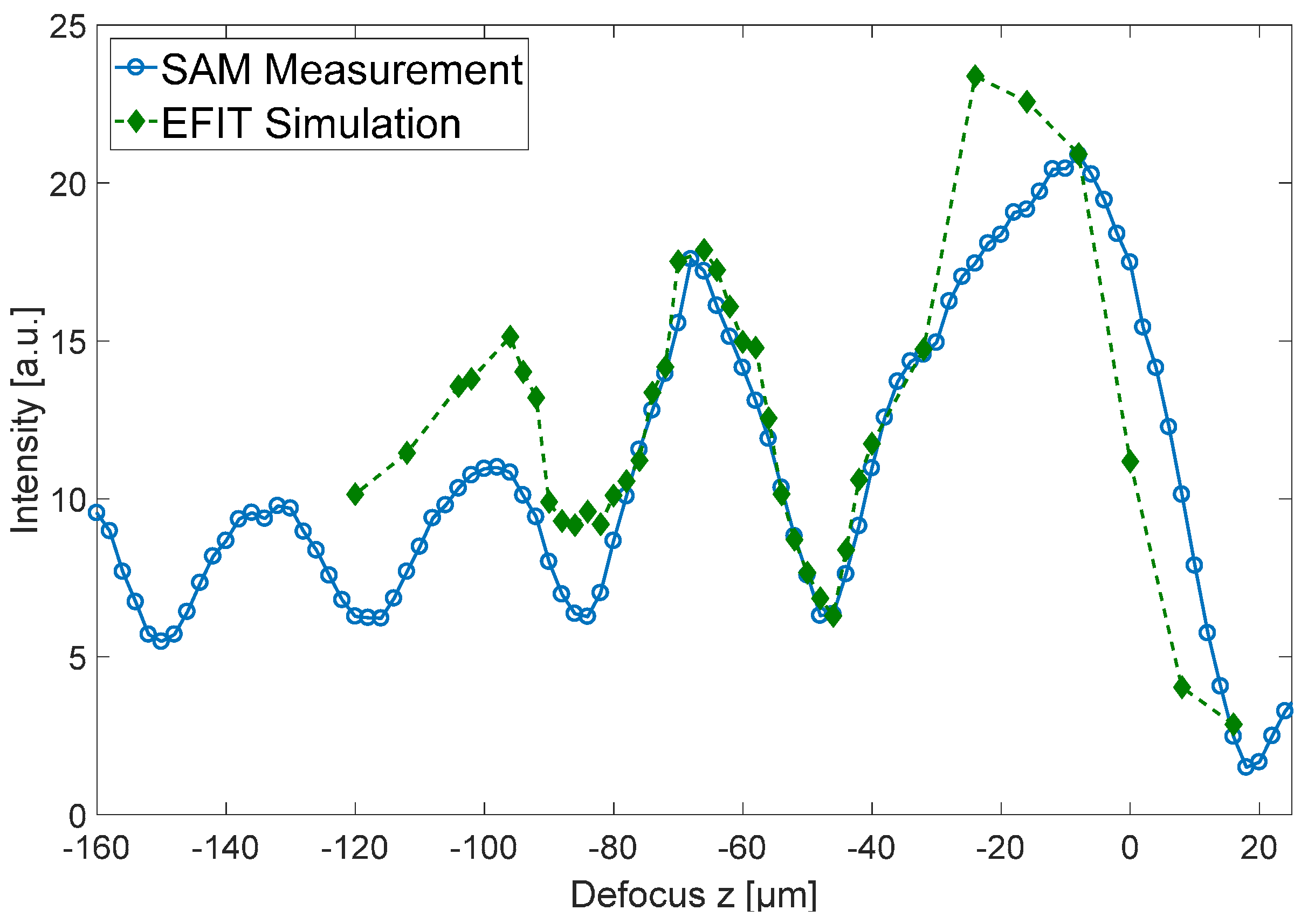
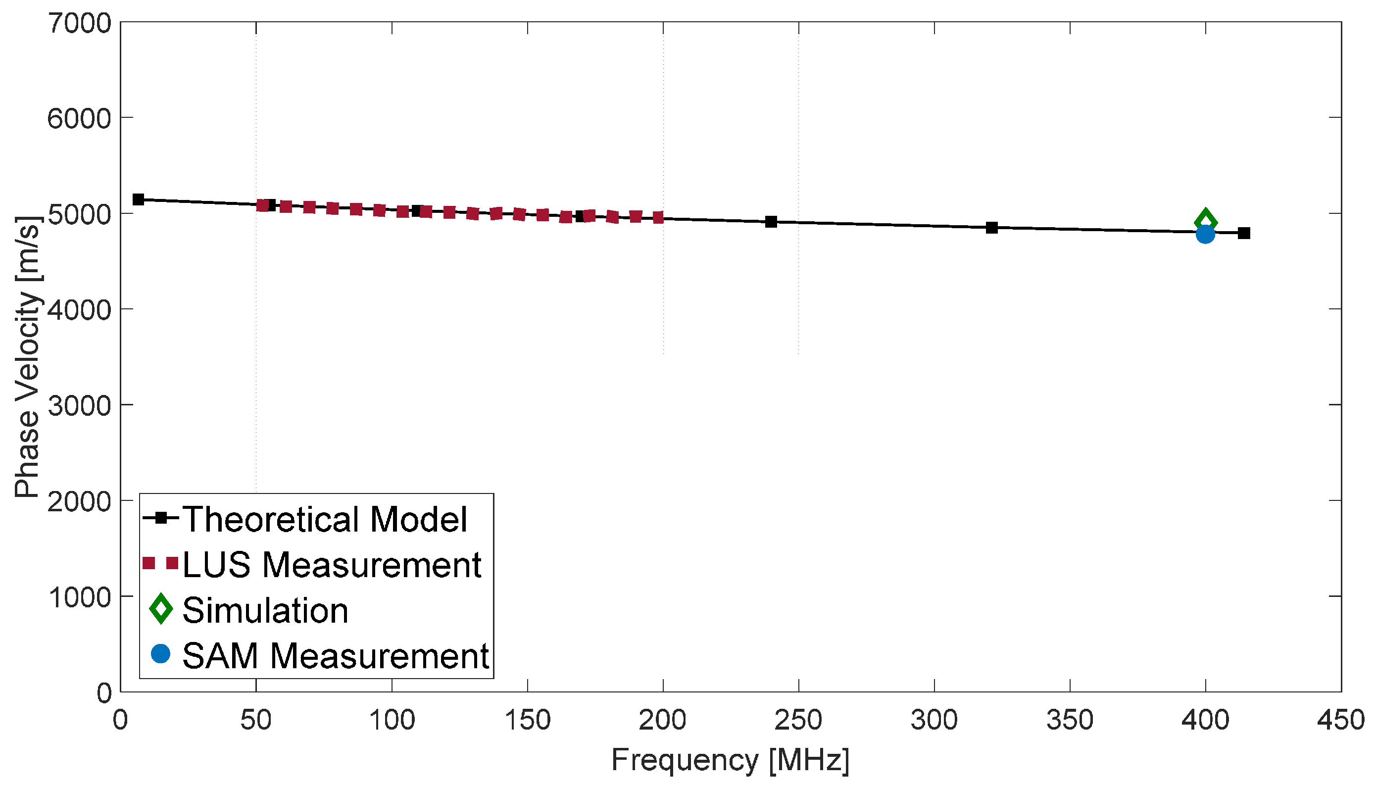
3.2. Aluminium Thin Film on Silicon Substrate

Here, the simulation of I(z) on an aluminium coating with a thickness of approximately 1 µm on a silicon substrate (100) was performed. The simulated results are directly compared to the SAM measurement in Figure 7.
Figure 8 shows the Rayleigh phase velocity vR as function of frequency. The solid line corresponds to the theoretical model, predicting the Rayleigh dispersion curve of a 1 µm aluminium coating on a silicon substrate. The dotted line in the frequency range from 50 to 200 MHz was obtained by laser ultrasonic measurements, where good agreement was found. The empty diamond corresponds to the EFIT simulation result, and the full circle corresponds to the SAM measurement.
There is only one data point obtained from the SAM measurement and SAM simulation data because the measurement and simulation were performed in tone burst mode in order to obtain signals which are very narrow in the frequency domain (in our case at 400 MHz). The LUS measurement uses broadband acoustic surface waves in a frequency range from about 50 MHz to 200 MHz.
The wavelengths considered in this work are on the order of 10 µm. This means that they do penetrate the coating and their propagation is influenced by the substrate. However, the aluminium coating has a measurable influence on the phase velocity of the Rayleigh wave (see Figure 8).

4. Discussion and Conclusions

In this work, SAM I(z) measurements were simulated via EFIT, where (1) an aluminium bulk sample for calibration and (2) an aluminium-coated silicon wafer were analysed. From the I(z) curves, the Rayleigh wave velocity of samples (1) and (2) were determined. The simulated results were corroborated via non-destructive SAM and LUS measurements. The obtained results demonstrate that the presented approach is highly useful for the material characterization of coatings.
The results summarized in Table 1 and Table 2 give integer values for the I(z) periodicity Δz, because the SAM measurement is limited by the number of oscillations and the 2 µm steps of defocus positions. Moreover, the number of evaluable A-scans is restricted due to multi-reflected signals in the measurement and in the simulation. Nevertheless, the Rayleigh wave velocities evaluated via EFIT simulations and SAM measurements are corroborated via the LUS method. The error in the determined Rayleigh velocity of the LUS measurements lies in the range of ±10 m/s.
The advantages of the performed EFIT simulation tackle the challenges of state-of-the-art SAM measurements—namely, accurate data interpretation and the choice of the most suitable transducer. In addition, the most effective lens for a specific sample can be designed via EFIT simulation support.

Acknowledgments

The authors thank Jördis Rosc (MCL) for valuable discussions and Manfred Wießner (MCL) for the XRD measurements. PVA TePla Analytical Systems GmbH, (Westhausen, Germany) is gratefully acknowledged, especially Peter Czurratis, Peter Hoffrogge and Tatjana Djuric-Rissner for their contribution regarding the SAM equipment. This work has received funding from ENIAC Joint undertaking under FP7 research (No. 621270) and FFG (No. 843740) and partly from the EU, H2020 (No. 688225). Financial support by the Austrian Federal Government (in particular from Bundesministerium für Verkehr, Innovation und Technologie and Bundesministerium für Wissenschaft, Forschung und Wirtschaft) represented by Österreichische Forschungsförderungsgesellschaft mbH and the Styrian and the Tyrolean Provincial Government, represented by Steirische Wirtschaftsförderungsgesellschaft mbH and Standortagentur Tirol, within the framework of the COMET Funding Programme (No. 837900) is also gratefully acknowledged.

Author Contributions

Roland Brunner conceived and designed the experiments; Eva Grünwald (LUS&SAM), Philipp Aldo Wieser (SAM) and Robert Nuster (LUS) performed experimental work; René Hammer and Eva Grünwald performed simulations for the experimental work; Rudolf Zelsacher and Michael Ehmann manufactured the samples; Martin Hinderer and Ingo Wiesler developed the tone burst device for the SAM. Eva Grünwald and Roland Brunner wrote the paper.

Conflicts of Interest

The authors declare no conflict of interest.

References

  1. Grovenor, C.R.M. Microelectronic Materials; Plenum Press: New York, NY, USA, 1989. [Google Scholar]
  2. Zhang, F.; Kirshnaswamy, S.; Fei, D.; Rebinsky, D.A.; Feng, B. Ultrasonic characterization of mechanical properties of Cr- and W-doped diamond-like carbon hard coatings. Thin Solid Films 2006, 503, 250–258. [Google Scholar] [CrossRef]
  3. Neubrand, A.; Hess, P. Laser generation and detection of surface acoustic waves: Elastic properties of surface layers. J. Appl. Phys. 1992, 71, 227–238. [Google Scholar] [CrossRef]
  4. Schneider, D.; Witke, T.; Schwarz, T.; Schöneich, B.; Schultrich, B. Testing ultra-thin films by laser-acoustics. Surf. Coat. Technol. 2000, 126, 136–141. [Google Scholar] [CrossRef]
  5. Schneider, D.; Schwarz, T. A photoacoustic method for characterizing thin films. Surf. Coat. Technol. 1997, 91, 136–146. [Google Scholar] [CrossRef]
  6. Hurley, D.C.; Tewary, V.K.; Richards, A.J. Surface acoustic wave methods to determine the anisotropic elastic properties of thin films. Meas. Sci. Technol. 2001, 12, 1486–1494. [Google Scholar] [CrossRef]
  7. Briggs, G.A.D. Advances in Acoustic Microscopy, 2nd ed.; Plenum Press: New York, NY, USA, 1995. [Google Scholar]
  8. Yu, Z.; Boseck, S. Scanning acoustic microscopy and its applications to material characterization. Rev. Mod. Phys. 1995, 67, 863. [Google Scholar] [CrossRef]
  9. Grünwald, E.; Rosc, J.; Hammer, R.; Czurratis, P.; Koch, M.; Kraft, J.; Schrank, F.; Brunner, R. Automatized failure analysis of tungsten coated TSVs via scanning acoustic microscopy. Microelectron. Reliab. 2016, 64, 370–374. [Google Scholar] [CrossRef]
  10. Shin, S.W.; Yun, C.B.; Popovics, J.S.; Kim, J.H. Improved rayleigh wave velocity measurement for nondestructive early-age concrete monitoring. Res. Nondestruct. Eval. 2017, 18, 45–68. [Google Scholar] [CrossRef]
  11. Debboub, S.; Boumaïza, Y.; Boudour, A.; Tahraoui, T. Attenuation of Rayleigh surface waves in a porous material. Chin. Phys. Lett. 2012, 29, 044301. [Google Scholar] [CrossRef]
  12. Levy, M.; Bass, H.E.; Stern, R. Modern Acoustical Techniques for the Measurement of Mechanical Properties; Academic Press: San Diego, CA, USA, 2001. [Google Scholar]
  13. Tiersten, H.F. Elastic surface waves guided by thin films. J. Appl. Phys. 1969, 40, 770–789. [Google Scholar] [CrossRef]
  14. Farnell, G.W.; Adler, E.L. Elastic wave propagation in thin layers. Phys. Acoust. 1972, 9, 35–127. [Google Scholar] [CrossRef]
  15. Chimenti, D.E.; Nayfeh, A.H.; Butler, D.L. Leaky Rayleigh waves on a layered halfspace. J. Appl. Phys. 1982, 53, 170–176. [Google Scholar] [CrossRef]
  16. Liang, K.K.; Kino, G.S.; Khuri-Yakub, B.T. Material characterization by the inversion of V(z). IEEE Trans. Sonics Ultrason. 1985, 32, 213–224. [Google Scholar] [CrossRef]
  17. Ghosh, T.; Maslov, K.I.; Kundu, T. A new method for measuring surface acoustic wave speeds by acoustic microscopes and its application in characterizing laterally inhomogeneous materials. Ultrasonics 1997, 35, 357–366. [Google Scholar] [CrossRef]
  18. Bamber, M.J.; Cooke, K.E.; Man, A.B.; Derby, B. Accurate determination of Young’s modulus and Poisson’s ratio of thin films by a combination of acoustic microscopy and nanoindentation. Thin Solid Films 2001, 398, 299–305. [Google Scholar] [CrossRef]
  19. Comte, C.; Von Stebut, J. Microprobe-type measurement of Young’s modulus and Poisson coefficient by means of depth sensing indentation and acoustic microscopy. Surf. Coat. Technol. 2002, 154, 42–48. [Google Scholar] [CrossRef]
  20. Weglein, R.D. A model for predicting acoustic material signatures. Appl. Phys. Lett. 1979, 34, 179–181. [Google Scholar] [CrossRef]
  21. Henry, L.B. Ray-optical evaluation of V(z) in the reflection acoustic microscope. IEEE Trans. Sonics Ultrason. 1984, 31, 105–116. [Google Scholar]
  22. Kim, J.N. Multilayer Transfer Matrix Characterization of Complex Materials with Scanning Acoustic Microscopy. Master’s Thesis, The Pennsylvania State University, Pennsylvania, PA, USA, 2013. [Google Scholar]
  23. Guddati, M.N.; Yue, B. Modified integration rules for reducing dispersion error in finite element methods. Comput. Methods Appl. Mech. Eng. 2004, 193, 275–287. [Google Scholar] [CrossRef]
  24. Willberg, C.; Duczek, S.; Perez, J.M.V.; Schmicker, D.; Gabbert, U. Comparison of different higher order finite element schemes for the simulation of Lamp waves. Comput. Methods Appl. Mech. Eng. 2012, 241, 246–261. [Google Scholar] [CrossRef]
  25. Ham, S.; Bathe, K.J. A finite element method enriched for wave propagation problems. Comput. Struct. 2012, 94, 1–12. [Google Scholar] [CrossRef]
  26. Komatitsch, D.; Vilotte, J.-P. The spectral element method, an efficient tool to simulate seismic response. Bull. Seismol. Soc. Am. 1998, 88, 368–392. [Google Scholar]
  27. Zampieri, E.; Pavarino, L.F. Approximation of acoustic waves by explicit Newmark’s schemes and spectral element methods. J. Comput. Appl. Math. 2006, 185, 308–325. [Google Scholar] [CrossRef]
  28. Fornberg, B. The pseudospectral method comparisons with finite differences for the elastic wave equation. Geophysics 1987, 52, 483–501. [Google Scholar] [CrossRef]
  29. Zhao, Z.; Xu, J.; Horiuchi, S. Differentiation operation in the wave equation for the pseudospectral method with a staggered mesh. Earth Planets Space 2001, 53, 327–332. [Google Scholar] [CrossRef]
  30. LeVeque, R.J. Wave propagation algorithms for multidimensional hyperbolic systems. J. Comput. Phys. 1997, 113, 327–353. [Google Scholar] [CrossRef]
  31. Virieux, J. SH-wave propagation in heterogeneous media: Velocity-stress finite-difference method. Geophysics 1984, 49, 1933–1942. [Google Scholar] [CrossRef]
  32. Graves, R.W. Simulating seismic wave propagation in 3D elastic media using staggered-grid. Bull. Seismol. Soc. Am. 1996, 86, 1091–1106. [Google Scholar]
  33. Pitarka, A. 3D elastic finite-difference modeling of seismic motion using staggered grids with nonuniform spacing. Bull. Seismol. Soc. Am. 1999, 89, 54–68. [Google Scholar]
  34. Saenger, E.H.; Gold, N.; Shapiro, S.A. Modeling the propagation of elastic waves using a modified finite-difference grid. Wave Motion 2000, 31, 77–92. [Google Scholar] [CrossRef]
  35. Fellinger, P.; Marklein, R.; Langenberg, K.J.; Klaholz, S. Numerical modeling of elastic wave propagation and scattering with EFIT–elastodynamic finite integration technique. Wave Motion 1995, 21, 47–66. [Google Scholar] [CrossRef]
  36. Schubert, F.; Köhler, B. Time domain modelling of axisymmetric wave propagation in isotropic elastic media with CEFIT–cylindrical elastodynamic finite integration technique. J. Comput. Acoust. 2001, 9, 1127–1146. [Google Scholar]
  37. Taflove, A.; Hagness, S.C. Computational Electrodynamics: The Finite-Difference Time-Domain Method; Artech House: Boston, MA, USA, 2005. [Google Scholar]
  38. Hammer, R.; Pötz, W.; Arnold, A. Single-cone real-space finite difference scheme for the time-dependent Dirac equation. J. Comput. Phys. 2014, 265, 50–70. [Google Scholar] [CrossRef]
  39. Grünwald, E.; Hammer, R.; Rosc, J.; Maier, G.A.; Bärnthaler, M.; Cordill, M.J.; Brand, S.; Nuster, R.; Krivec, T.; Brunner, R. Advanced 3D failure characterization in multi-layered PCBs. NDT E Int. 2016, 84, 99–107. [Google Scholar] [CrossRef]
  40. Royer, D.; Dieulesaint, E. Elastic Waves in Solids. I. Free and Guided Propagation; Springer: Berlin, Germany, 2000. [Google Scholar]
Figure 1. Schematic of scanning acoustic microscopy (SAM) principle.
Coatings 07 00230 g001
Figure 2. The staggered discretization of field variables velocity v and stress σ in the elastodynamic finite integration technique (EFIT).
Coatings 07 00230 g002
Figure 3. EFIT simulation of SAM measurement, time steps 1–9.
Coatings 07 00230 g003
Figure 4. Schematic of laser-induced ultrasound (LUS) set-up; CW laser denotes a continuous wave laser, SAW denotes a surface acoustic wave.
Coatings 07 00230 g004
Figure 5. LUS measurement on bulk aluminium. Comparison of EFIT result to LUS measurement.
Coatings 07 00230 g005
Figure 6. EFIT simulation (diamonds) and SAM measurement (circles) of I(z) for the aluminium bulk sample at 430 MHz.
Coatings 07 00230 g006
Figure 7. EFIT simulation (diamonds) and SAM measurement (circles) of I(z) for an aluminium coating on silicon sample at 400 MHz.
Coatings 07 00230 g007
Figure 8. Rayleigh wave velocity as function of frequency for a 1 µm aluminium coating on silicon.
Coatings 07 00230 g008
Table 1. Rayleigh wave velocity results for an aluminium sample.
MethodΔz (µm)vR (m/s)
EFIT132896
SAM132896
LUS2969
Literature [7]2906
Table 2. Rayleigh wave velocity results at 400 MHz for 1 µm aluminium coating on silicon.
MethodΔz (µm)vR (m/s)
EFIT384775
SAM404899
Theoretical Model4819

