1. Introduction
Flame deposition has been in commercial use for several decades because it is a quick and effective way of creating a protective and adhesive coating on a surface. An early description of the process is provided by Towler [
1]. Zhang
et al. [
2] studied heat transfer from an air/propane or air/acetylene flame to polymer particles injected into the flame. This process has been used for some years to apply a polymer coating to metal surfaces. In this process, shown schematically in
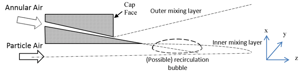
Figure 1, the polymer powder is injected into the flame using an air stream. The goal of the process is to heat the ground polymer enough to soften it without overheating it, which would cause it to burn. The jet then carries the softened polymer particles to a metal surface, itself heated by the same flame, to which they adhere forming a continuous protective coating. The gun head shown in
Figure 1, and schematically in a longitudinal section in
Figure 2, is the origin of the jets. Some of the details of the gun head design are proprietary. This particular gun head includes an annular jet and a central jet with its nozzle staggered relative to the annular jet orifice. Critical gun head dimensions are given in
Table 1. In practice, the central jet is the particle bearing air stream and the air only concentric annular jet around it is the main momentum source. The gun head includes pinhole sized fuel (propane) ports, arranged in two circles concentric with the two inner jets. In this study we only modelled an isothermal concentric jet flow, by shutting off the propane and particle sources. The goal of this study was to try to develop an effective computational fluid dynamics (CFD) model using the Reynolds Averaged Navier Stokes (RANS) models in Fluent, with Gambit as a preprocessor, and validate it with experimental data. Such a model would be the basis for subsequent more complex CFD models. These more advanced models would include first the particles in the central jet and then the particles and carbon dioxide (CO
2) in place of the propane, so the effect of the particles on the mixing of the air and propane would be modelled. In both advanced cases suitable experimental data would be gathered for comparison with the CFD models.
The two most fundamental variables that determine the flow field created by a coaxial jet, or in this case the gun head, are the design of the gun head and the velocities of the jets. Early papers considered the fundamentals of the design of a nozzle creating a coaxial jet. One of several fundamental variables altering the flow field of a coaxial jet is whether the flow leaving each nozzle is fully developed. Two early papers on coaxial jets, Chigier and Beer [
3] and Champagne and Wygnanski [
4] do not address this point, but a careful reading of both papers makes it clear that the jets were not fully developed in either body of work. However, Chigier and Beer [
3] point out a second fundamental variable altering the flow field. The flow field of a coaxial jet depends not only on the velocity of both jets and their nozzle diameters, but also the spacing, if any, between the inner round jet and the concentric annular jet. Champagne and Wygnanski [
4] also point out the radius of both jets alters the flow field. Chigier and Beer [
3] further point out that a coaxial jet flow field is a combination of two flow fields, that of a single round jet and that of an annular jet.
The staggering of the central and annular nozzles in the gun head shown in
Figure 2 is an extremely important feature of the gun head used in this work that is not present in any of the coaxial jets described in the literature. In all coaxial jet studies found in the literature, the origins of both jets are in the same plane. In contrast, the extension of the central channel in the nozzle used in this work results in the origin of the central jet being about 1.4 cm downstream of the origin of the annular air jet. The outer surface of this extension is tapered ending with a sharp edge at the plane of confluence of the central and annular jets. The angle of the truncated cone is shallow enough to ensure the annular air jet remains attached to the outer surface of this extension. This design feature causes the annular jet to have some momentum directed towards the flow axis. The gun head used in this work, in combination with the rest of the apparatus, creates a fully developed central jet but does not create a fully developed annular air jet.
Figure 1.
Schematic diagram of the basic apparatus (arrows show the flow direction).
Figure 1.
Schematic diagram of the basic apparatus (arrows show the flow direction).
Figure 2.
Schematic longitudinal section through a radius of the gun head. (The horizontal dashed line is the centerline of the jet. The plane z = 0 is located at the cap face. This plane contains the origin of the annular air jet).
Figure 2.
Schematic longitudinal section through a radius of the gun head. (The horizontal dashed line is the centerline of the jet. The plane z = 0 is located at the cap face. This plane contains the origin of the annular air jet).
Table 1.
Critical dimensions of the gun head.
Table 1.
Critical dimensions of the gun head.
| Critical Dimension | Diameter of Gun Head (mm) | Approximate Length of Truncated Central Cone (mm) | Diameter of Central Jet (mm) | Annular Jet Nozzle Gap (mm) |
|---|
| Experiment 1 | 76 | 14 | 9.5 | 0.38 |
| Experiment 2 | 0.32 |
| Experiment 3 | 0.27 |
One flow rate was chosen for each of the two jets. Then, the three different ratios of the linear momentum of the annular air jet to the central jet shown in
Table 2 were chosen. It is important to realize that the staggering of the two nozzles, shown in
Figure 2, means that the annular jet must slow significantly as it travels from its origin to the tip of the central nozzle, through the ambient air, before it begins to merge with the central jet. As long as the velocity ratio at the origin of the central jet is low enough, regardless of the average velocity ratio at the jet origins, there will be no recirculation zone formed in the near field of the jet. The extension of the central channel past the origin of the annular air jet allows the annular flow to have a much larger mass and velocity compared to the central jet than would otherwise be possible without causing a recirculation zone. Such a zone, centered on the jet axis, has been found to trap some of the polymer particles and increase their radius of distribution when the process is used for commercial purposes.
Table 2.
The annular and central air jet properties used for experimental work.
Table 2.
The annular and central air jet properties used for experimental work.
| Variable | Experiment 1(E1) | Experiment 2(E2) | Experiment 3(E3) |
|---|
| Annular Air Jet Flow Rate (m3/min) | 0.1 |
| Central Air Jet Flow Rate (m3/min) | 0.04 |
| Central Air Jet Momentum (N) | 7.52 × 10⁻³ |
| Central Air Jet Average Nozzle Velocity (m/s) | 9.4 |
| Annular/Central Air Jet Momentum Ratio | 25 | 30 | 35 |
| Annular Air Jet Average Nozzle Velocity(m/s) | 106 | 127 | 148 |
Chigier and Beer [
3] began examination of coaxial jets by increasing the momentum of the central jet from zero. This method allowed study of the changes caused by the increasing strength of the central jet to the toroidal shaped recirculation zone, with its axis on the centerline of the jet, that was created by the annular air jet alone. As the annular to central jet velocity ratio decreased to 2.35, this torus was increasingly squeezed between the central and annular air jets and a second torus with rotation opposite the first torus formed. The distance between the radius of the central jet and the inner diameter of the annular jet of 1.95 cm also played a role in the continuation of the toroidal recirculation zone. It was still present at an annular to central jet velocity ratio of 0.117. Chigier and Beer's work was extended by Ko and Kwan [
5] and Ko and Au [
6] who identified three regions in a coaxial jet. They are an initial zone to the end of the core of the central or annular jet, whichever is shorter, an intermediate zone in which the jets become fully mixed, and a fully merged zone in which the jets behave as though they were one jet originating from a circular nozzle. Ko and Kwan [
5] also found the central and annular jets were fully merged at 6 diameters downstream from the nozzle where, once again, the axial velocity profile was similar to that of a single jet.
Ko and Kwan [
5] found that near the nozzle the turbulence intensity was lowest within the core of each jet, where there had been no mixing and the air was at its nozzle velocity. Within the layers resulting from the mixing of each jet with surrounding stationary air, the turbulence intensity increased rapidly. Ribeiro and Whitelaw [
7] reported the same result. Further downstream, the three layers of high turbulence intensity merged into one jet with only the one mixing layer. Ko and Kwan [
5] also found the time averaged pressure in the flow field was not uniform and it changed with the velocity ratio of the jets.
Buresti
et al. [
8] studied, amongst other flow features, the comparative magnitudes of the time varying part of the axial and radial velocities in the inner and outer mixing layers within two central nozzle diameters downstream from the nozzle. It was found that they were a result of the 5 mm spacing between the annular and central jets which can be thought of as a bluff body that produces a wake. This feature was not present in the current work because of the near knife edge thickness of the tip of the nozzle at the central jet origin.
Rehab
et al. [
9] studied water jets, not air jets, with a knife edge separating the origins of the two jets. They found that a critical annular jet to central jet velocity ratio existed beyond which a recirculation zone developed just downstream of the nozzle on the jet axis. Rehab
et al. [
9] point out that the vortices that formed in the mixing layers around each jet caused most of the entrainment in both jets. Their work also showed that the critical annular jet to central jet velocity ratio necessary for the formation of the axial recirculation zone is a minimum of about 8. The recirculation zone downstream end was at the merging point of the mixing layers around the annular jet and the inner jet.
Buresti
et al. [
10] also published a second paper, a detailed examination of the near field of a coaxial jet using two different velocity ratios. They created a second nozzle, in addition to the nozzle with a 5 mm spacing between the radius of the central jet and the annular jet. This second nozzle had a knife edge between the radius of the central jet and the annular jet. Both nozzles were used with both velocity ratios and allowed additional examination of the effect of the spacing between the central jet and the annular jet. Buresti
et al. [
10] mapped the entire flow field and found that at the higher velocity ratio, with the annular jet dominant, changing the spacing between the jets from 5 mm to a razor edge caused a large decrease in the time varying part of the radial velocity and a large decrease in the time varying part of the shear stresses too. This difference diminished with axial distance downstream and was gone when the flow reached a downstream distance of about half the diameter of the central jet. The near knife edge of the tip of the central jet origin means that the jet studied here is closer to the nozzle used by Buresti
et al. [
10] with a knife edge between the central and annular jet.
3. Numerical Modelling
Five generations of meshes were created for numerical modelling. The first two generations, Grid1 and Grid2, were discarded because these meshes gave unsatisfactory results. Numerical simulations of all three experiments were performed using a variety of meshes from subsequent generations and a variety of turbulence models, with some variations in boundary conditions as will be explained later. The agreement between simulations and experiment was found to be substantially the same for all three experiments. Consequently, most of the results shown are for Experiment 1 with a few for Experiment 2.
3.1. General Meshing Features
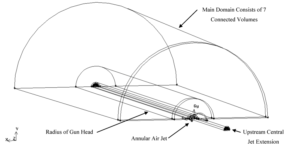
Numerical modeling used a commercially available CFD package Fluent 6.3.26 with Gambit 2.4 for geometry and meshing. The rotational symmetry of the axisymmetric jets and periodically arranged propane holes allowed the creation of three types of domain with three wedge angles: 60° (wedge), 180° (semicircular) and 360° (full circle). These grid families are designated as Grid3, Grid4, and Grid5 respectively in the following pages. As an example, the semicircular domain (Grid4) is shown in
Figure 10 and the critical domain dimensions given in
Table 3. The
x,
y, and
z axes for the domain are shown in the lower left. The
z axis lies on the jet axis and the origin lies on the plane of the origin of the annular jet, the upstream end of the main domain. Note that the propane jets have been removed for this analysis. All domains have the same radius of 0.13 m at the inlet, increasing linearly to 0.143 m at the outlet. In most cases a domain length of 0.6 m was used. The inlet boundary conditions in this numerical study match the three experiments outlined in
Table 2 in the previous section, with the annular air jet to central jet momentum ratios of 25, 30 and 35 for the Experiments E1, E2 and E3, respectively. Most of the data presented here are for the momentum ratio of 25.
Figure 10.
Flow domain for Grid 4 (the semi-circular case).
Figure 10.
Flow domain for Grid 4 (the semi-circular case).
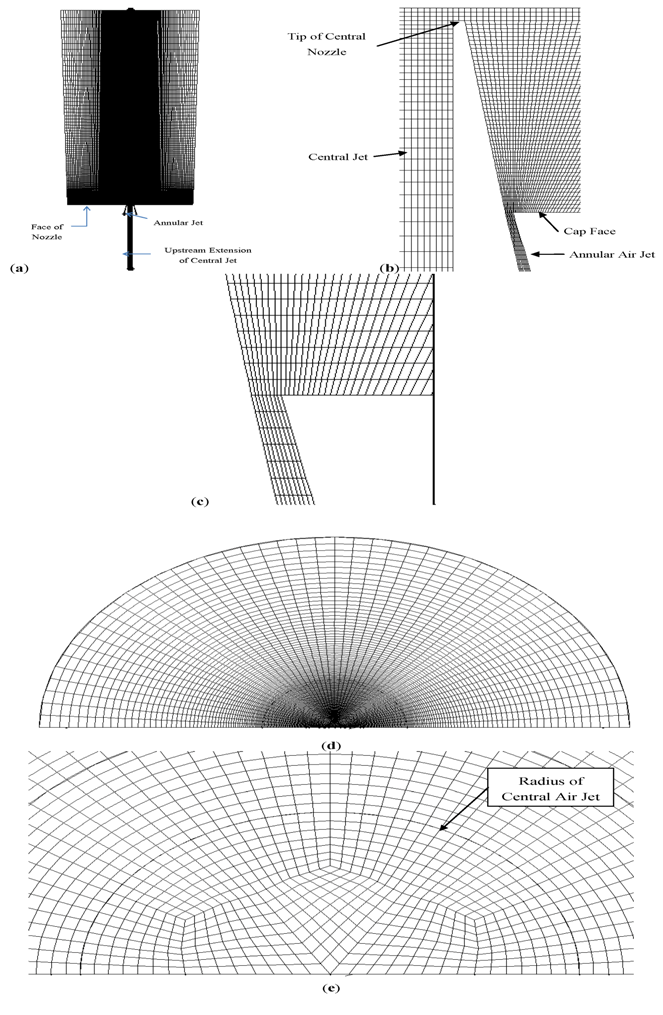
Substantial effort was put into creating meshes with elements as orthogonal as possible. To that end, only the core, central region is covered by semi-structured Cooper type hexagonal elements, while all other sections are meshed by structured hexagonal elements. Due to the vast range of length scales, the size of the control volumes varied widely. The number of control volumes also varied widely in order to resolve high gradient zones in an optimal way.
Figure 11a–e illustrates details of a mesh for the domain with a semi-circular cross-section. The core area elements of
Figure 11a are too fine to be resolved on the scale used. Consequently,
Figure 11b,c is a close-up of critical areas, the origins of the jets. The same is true of the bottom center of
Figure 11d, which is the center of the jet.
Figure 11e shows this region in detail. Overall, the extremely wide range of length scales posed a significant challenge in generating properly adapted meshes.
Figure 11c,e illustrates the difficulty of trying to mesh very small dimensions and circular dimensions respectively with regular hexagonal mesh. In spite of this difficulty all domains were divided into connected volumes and meshed using structured mesh, except the near-axis region that had to be meshed by Cooper mesh. A list of meshes used in this study with main resolution parameters is shown in
Table 3.
Figure 11.
Grid 4 NP_E1 Mesh (
a) Horizontal plane of symmetry (The mesh is too fine to be resolved on this scale in the solid black area); (
b) Close up of the mesh at the origins of the central and annular jets in the horizontal plane of symmetry (dimensions given in
Table 1); (
c) Close up of the mesh at the origin of the annular jet in the horizontal plane of symmetry (dimensions given in
Table 1); (
d) Downstream domain end mesh; (
e) Core of domain shown in (d)
Table 3.
A list of meshes used in the study, with key resolution parameters.
Table 3.
A list of meshes used in the study, with key resolution parameters.
| Grid name(these names are used in subsequent text and plots) | Domain wedge angle [deg] | Domain Length (m) | Elements around circumference | Cells across (Radial × Axial) | Total number of control volumes |
|---|
| Central (PA) jet | Annular(AA) jet | Outside of PA and AA jets |
|---|
| Grid3_60_NP_E2_VC | 60 | 0.60 | 16 | 15 × 72 | 8 × 70 | 139 × 162 | 361,568 |
| Grid3_60_NP_E1_VC_2 | 60 | 0.60 | 12 | 11 × 70 | 8 × 70 | 97 × 152 | 180,336 |
| Grid3_60_NP_E2_VC_2 | 60 | 0.60 | 12 | 11 × 70 | 8 × 70 | 97 × 152 | 180,336 |
| Grid3_60_NP_E3_VC_2 | 60 | 0.60 | 12 | 11 × 70 | 8 × 70 | 97 × 152 | 180,336 |
| Grid3_60_NP_E1_VC_2L | 60 | 1.0 | 12 | 11 × 70 | 8 × 70 | 97 × 228 | 256,944 |
| Grid3_60_NP_E2_VC_2L | 60 | 1.0 | 12 | 11 × 70 | 8 × 70 | 97 × 228 | 256,944 |
| Grid3_60_NP_E1_VC_2R | 60 | 0.60 | 12 | 11 × 140 | 8 × 70 | 97 × 266 | 315,648 |
| Grid3_60_NP_E2_VC_2R | 60 | 0.60 | 12 | 11 × 140 | 8 × 70 | 97 × 266 | 315,648 |
| Grid3_60_NP_E1_VC_2S | 60 | 0.50 | 12 | 26 × 500 | 7 × 90 | 235 × 1030 | 7.770,880 |
| Grid3_60_NP_E2_VC_2S | 60 | 0.50 | 12 | 26 × 500 | 7 × 90 | 235 × 1030 | 7.770,880 |
| Grid3_60_NP_E1_VC_2T | 60 | 0.60 | 12 | 11 × 140 | 8 × 70 | 154 × 266 | 497,592 |
| Grid3_60_NP_E2_VC_2T | 60 | 0.60 | 12 | 11 × 140 | 8 × 70 | 154 × 266 | 497,592 |
| Grid3_60_NP_E2_C | 60 | 0.60 | 20 | 18 × 102 | 12 × 100 | 148 × 214 | 645,920 |
| Grid3_60_NP_E1_M | 60 | 0.60 | 32 | 26 × 145 | 16 × 140 | 201 × 290 | 1,920,416 |
| Grid3_60_NP_E2_M | 60 | 0.60 | 32 | 26 × 145 | 16 × 140 | 201 × 290 | 1,920,416 |
| Grid3_60_NP_E3_M | 60 | 0.60 | 32 | 26 × 145 | 16 × 140 | 201 × 290 | 1,920,416 |
| Grid4_NP_E1 | 180 | 0.60 | 48 | 15 × 72 | 8 × 70 | 149 × 162 | 1,162,464 |
| Grid4_NP_E2 | 180 | 0.60 | 48 | 15 × 72 | 8 × 70 | 149 × 162 | 1,162,464 |
| Grid4A_NP_E1 | 180 | 0.60 | 48 | 15 × 110 | 8 × 70 | 149 × 235 | 1,670.544 |
| Grid4B_NP_E1 | 180 | 0.60 | 72 | 23 × 110 | 12 × 98 | 223 × 348 | 5,558,544 |
| Grid4C_NP_E1 | 180 | 0.60 | 72 | 23 × 110 | 12 × 98 | 223 × 238 | 3,839,904 |
| Grid4D_NP_E1 | 180 | 0.60 | 72 | 32 × 110 | 12 × 98 | 232 × 238 | 3,960,964 |
| Grid5_NP_E2_C | 360 | 0.60 | 64 | 16 × 49 | 9 × 94 | 135 × 148 | 1,296,768 |
| Grid5_NP_E2 | 360 | 0.60 | 88 | 21 × 69 | 12 × 133 | 183 × 203 | 3,324,024 |
| Grid5_NP_E2_F | 360 | 0.60 | 144 | 32 × 110 | 15 × 108 | 255 × 238 | 8,727,264 |
3.2. Domain Choice
The creation of the flow domains was governed by several requirements. First, different wedge angles were needed not only to use the Reynolds Averaged Navier Stokes (RANS) models presented in this study, but also to allow for subsequent Large Eddy Simulation (LES) modeling. Second, the slight flaring of the domain envelope allowed a smooth transition from a highly non-uniform mesh in the radial direction at the gun face to a more uniform mesh in the radial direction at the outlet. Third, the central jet was extended upstream to duplicate the experimental conditions and ensure that the flow in the central jet was fully developed by the time the air flowing through it reached the nozzle. In contrast, the annular jet channel was much shorter and did not allow for a fully developed velocity profile at its nozzle, again duplicating the experimental setup.
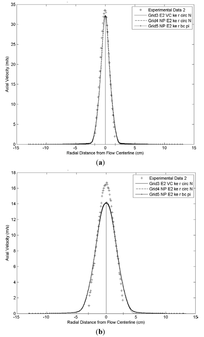
The different wedge angles are expected to provide identical results in theory. However, in complex domains and flow fields like the one studied here, such an assumption should be demonstrated by numerical experiment as well. There are subtle differences between the three domain shapes, especially since the mesh is not entirely structured, because it has a Cooper mesh core.
Figure 12 shows the axial velocity plots for three meshes, one each of Grid3, Grid4 and Grid5 families, all summarized in
Table 3. The particular meshes from each family were chosen to have a similar mesh density. The comparison of the velocity profiles confirm that the results are not affected by the wedge angle choice.
Figure 12.
Axial velocity
vs. radius (
a) at 10 cm (comparison of results for the three grid families.The legend entries refer to
Table 3); (
b) at 20 cm (comparison of results for the three grid families. The legend entries refer to
Table 3).
Figure 12.
Axial velocity
vs. radius (
a) at 10 cm (comparison of results for the three grid families.The legend entries refer to
Table 3); (
b) at 20 cm (comparison of results for the three grid families. The legend entries refer to
Table 3).
3.3. Boundary Conditions
Boundary conditions were chosen to reproduce the physical flow conditions as closely as possible. The proper specification of the upstream and the entrainment boundary conditions is more important than the specification of the outlet boundary conditions, since the upstream and circumferential boundary conditions influence the flow development downstream, throughout the flow domain modeled.
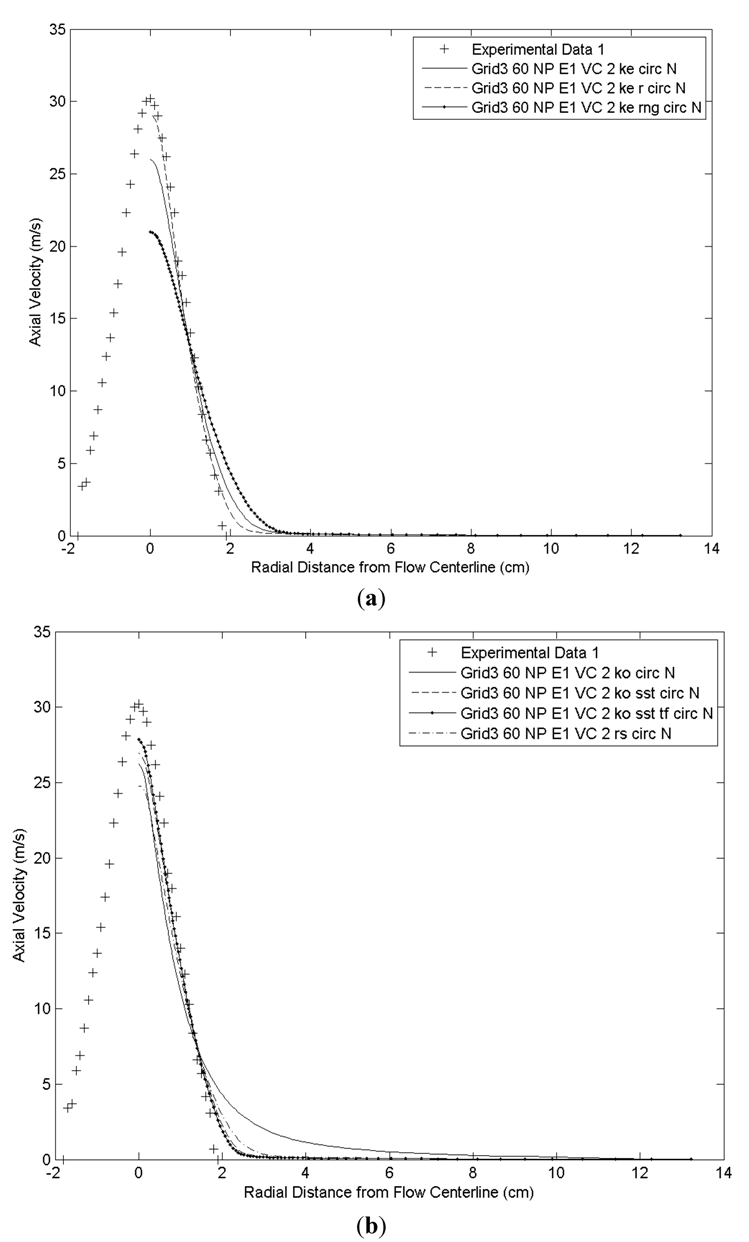
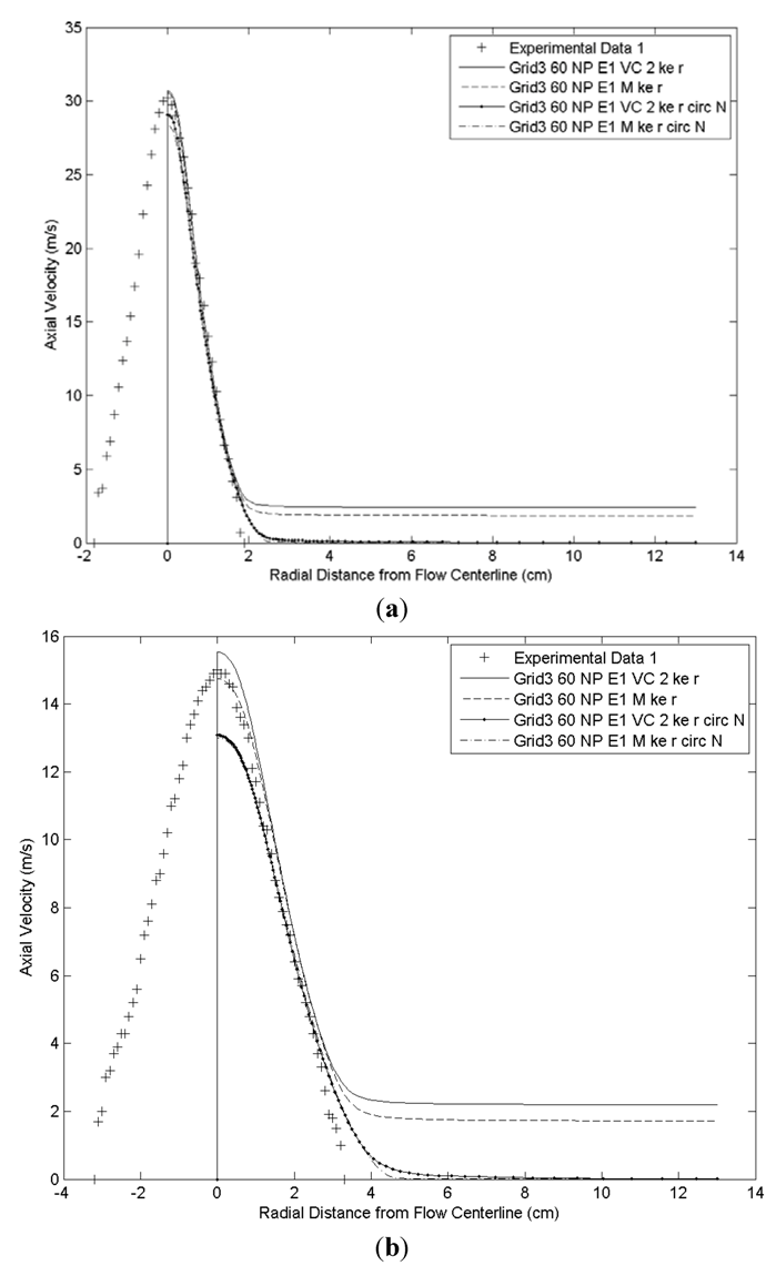
All simulations used velocity inlets as boundary conditions for both jets and the pressure outlet boundary condition at all other boundaries. Initially the pressure boundary velocity direction was specified to match the velocity vector of the adjacent cell center. The alternative option of forcing the boundary velocity vector to be perpendicular to the boundary was considered unphysical since the entrainment boundary surface was not parallel to the flow axis. However, this original choice introduced a significant error in the far field. The error caused by these boundary conditions is shown in the axial velocity plots presented in
Figure 13a,b for the coarsest and finest meshes of the Grid3 family. It is clear in these plots that the axial velocity is nonzero outside the jets and its magnitude depends on the mesh density. When the backflow direction specification method was changed to force the boundary velocity to be perpendicular to the boundary, the axial velocity outside the jet vanished. Strictly speaking, the proper boundary condition for the entrainment of stagnant air into the jet is to force the velocity vector to be perpendicular to the jet axis and not to be perpendicular to the boundary if the boundary is not parallel to the axis. However, in this work the angle between the boundary and the axis is only 1.2°, too small to produce a noticeable error.
Figure 13a,b also shows the result of making this change. All other results shown in this paper used this correct boundary condition.
Most models used the default settings within Fluent for turbulence at all boundaries. Changing these values had no effect on the converged flow field. The default setting of wall functions was also used to model boundary layers.
Figure 13.
Experiment 1: (
a) the effect of changing the circumferential boundary condition on the simulated flow field at 10 cm from the origin of the annular air jet (The legend entries refer to
Table 3. The “circ N” designator indicates the simulation used the correct boundary condition.); (
b) the effect of changing the circumferential boundary condition on the simulated flow field at 20 cm from the origin of the annular air jet (The legend entries refer to
Table 3).
3.4. Mesh Density Influence
Various mesh densities have been listed in
Table 3. In this section the influence of mesh density on numerical accuracy is examined.
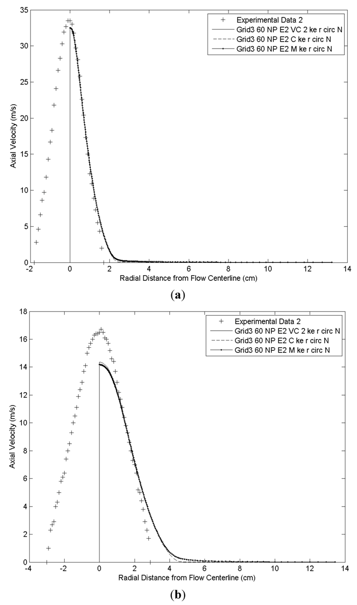
Figure 14 compares the velocity profiles obtained by modeling the Experiment E2 on three grids using approximately 180,000, 360,000 and 1,900,000 nodes each, with the k-ε realizable turbulence model and first order upwind discretization. The finest mesh had 10.6 times more control volumes than the coarsest mesh. The graphs show that all simulations give substantially the same results although there are minor differences in the velocity profiles at the centerline, at the 20 cm cross-section. Overall, it is clear from these results that even the coarsest mesh produces essentially grid independent results. It is also interesting that even with the first order differencing the presence of numerical diffusion is barely noticeable. The absence of numerical diffusion is due to the careful mesh alignment with the velocity field, something that is not always possible, but was attainable in this case.
3.5. Turbulence Model Influence
The question of which turbulence model gives the best agreement with experiment is best answered by numerical experiments. The flow field modeled here is dominated by mixing layers between the stagnant outside air and the annular jet, as well as between the annular jet and the central round jet, the two having very high velocity and momentum ratios. An additional specific feature of this flow is the presence of a conical solid surface that serves as the inner boundary for the annular air jet after it has exited its nozzle until it comes into contact with the much slower central round jet. For the most part, the flow features are determined by mixing, not by the wall boundary layer, except for the aforementioned zone between the origins of the two jets.
Figure 14.
Velocity profiles (a) at 10 cm from the origin of the annular air jet; (b) at 20 cm from the origin of the annular air jet.
Figure 14.
Velocity profiles (a) at 10 cm from the origin of the annular air jet; (b) at 20 cm from the origin of the annular air jet.
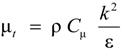
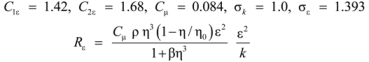
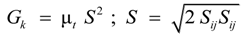
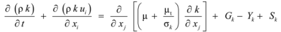
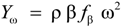
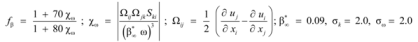
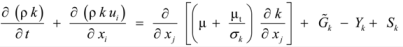
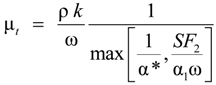
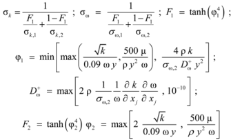
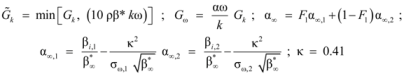
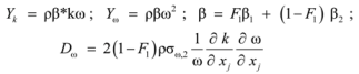
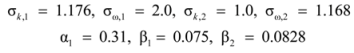
Three variations of the
k-ε model and three variations of the
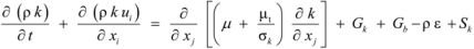
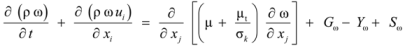
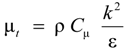
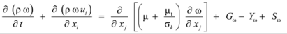
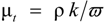
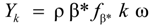
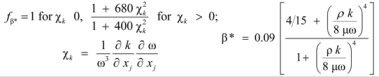
k-ω model and a Reynolds Stress model were used in comparison simulations to determine which of these agrees best with the experimental results. The equations used by the
k-ε and
k-ω turbulence models and their derivatives are shown in the
Appendix. The equations used by the Reynolds Stress model are omitted because of its poor agreement with experiment. The axial velocity profiles comparing different turbulence models are shown in
Figure 15a,b for the
z =2.5 cm cross section, in
Figure 16a,b for the
z = 5 cm cross section, in
Figure 17a,b for the
z = 10 cm cross section, and in
Figure 18a,b for the
z = 20 cm cross section.
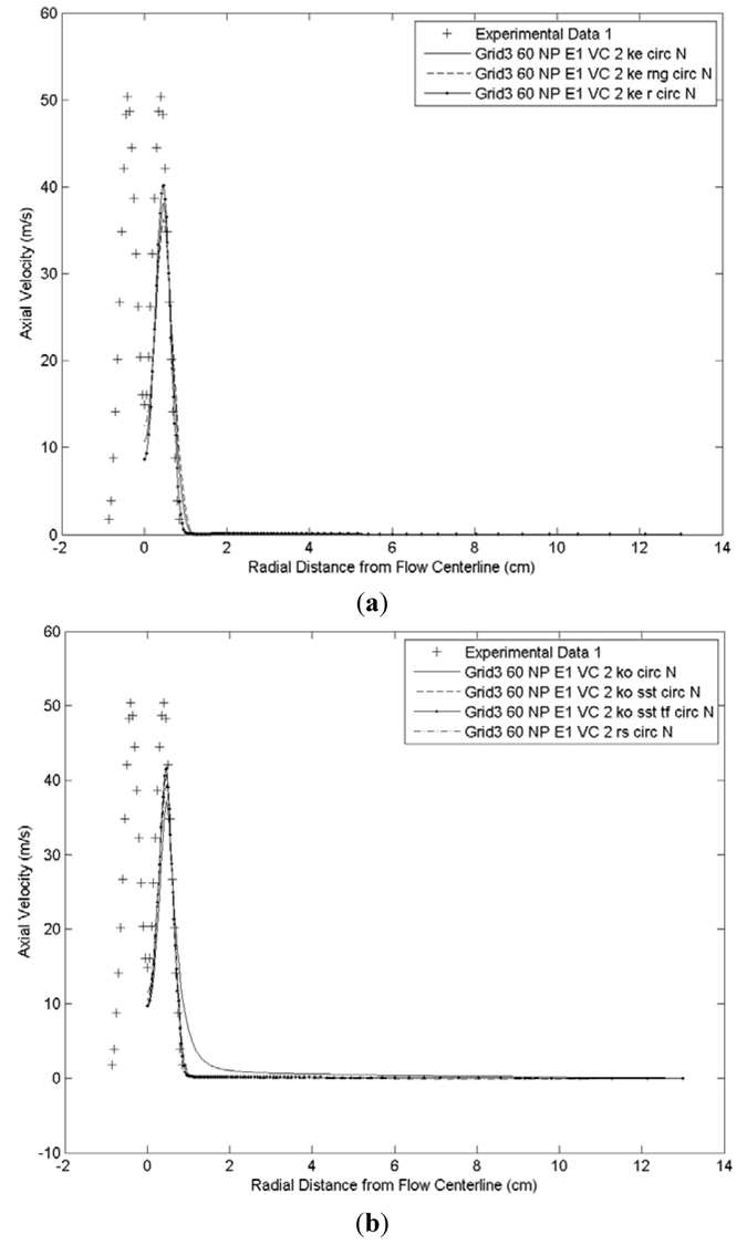
Figure 15.
Comparison with experiment of results from (a) standard k-ε (ke), k-ε realizable (ke r) and RNG k-ε (ke rng) models at z = 2.5 cm from the nozzle; (b) standard k-ω (ko), k-ω sst (ko sst), k-ω sst tf (ko sst tf) and the Reynolds Stress (rs) models at z = 2.5 cm from the nozzle.
Figure 15.
Comparison with experiment of results from (a) standard k-ε (ke), k-ε realizable (ke r) and RNG k-ε (ke rng) models at z = 2.5 cm from the nozzle; (b) standard k-ω (ko), k-ω sst (ko sst), k-ω sst tf (ko sst tf) and the Reynolds Stress (rs) models at z = 2.5 cm from the nozzle.
Figure 16.
Comparison with experiment of results from (a) standard k-ε (ke), k-ε realizable (ke r) and RNG k-ε (ke rng) models at z = 5 cm from the nozzle; (b) standard k-ω (ko), k-ω sst (ko sst), k-ω sst tf (ko sst tf) and the Reynolds Stress (rs) models at z = 5 cm from the nozzle.
Figure 16.
Comparison with experiment of results from (a) standard k-ε (ke), k-ε realizable (ke r) and RNG k-ε (ke rng) models at z = 5 cm from the nozzle; (b) standard k-ω (ko), k-ω sst (ko sst), k-ω sst tf (ko sst tf) and the Reynolds Stress (rs) models at z = 5 cm from the nozzle.
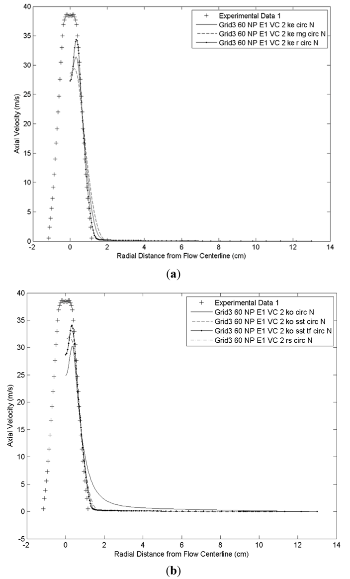
Figure 17.
Comparison with experiment of results from (a) standard k-ε (ke), k-ε realizable (ke r) and RNG k-ε (ke rng) models at z = 10 cm from the nozzle; (b) standard k-ω (ko), k-ω sst (ko sst), k-ω sst tf (ko sst tf) and the Reynolds Stress (rs) models at z = 10 cm from the nozzle.
Figure 17.
Comparison with experiment of results from (a) standard k-ε (ke), k-ε realizable (ke r) and RNG k-ε (ke rng) models at z = 10 cm from the nozzle; (b) standard k-ω (ko), k-ω sst (ko sst), k-ω sst tf (ko sst tf) and the Reynolds Stress (rs) models at z = 10 cm from the nozzle.
Figure 18.
Comparison with experiment of results from (a) standard k-ε (ke), k-ε realizable (ke r) and RNG k-ε (ke rng) models at z = 20 cm from the nozzle; (b) standard k-ω (ko), k-ω sst (ko sst), k-ω sst tf (ko sst tf) and the Reynolds Stress (rs) models at z = 20 cm from the nozzle.
Figure 18.
Comparison with experiment of results from (a) standard k-ε (ke), k-ε realizable (ke r) and RNG k-ε (ke rng) models at z = 20 cm from the nozzle; (b) standard k-ω (ko), k-ω sst (ko sst), k-ω sst tf (ko sst tf) and the Reynolds Stress (rs) models at z = 20 cm from the nozzle.
At the first cross section, 2.5 cm from the origin of the annular air jet, the results of all seven RANS models agree qualitatively with the experimental results. The central jet and the annular jet had not fully merged, so the maximum velocity was not located on the centerline of the gun head. However, the centerline velocity was still underpredicted. Comparison of the results of the standard k-ε model and its two derivatives with experimental results shows that k-ε realizable model results disagree the least with the maximum velocity while the k-ε rng model results disagree the least with the centerline velocity. Further comparison of the standard k-ω model, its two derivatives, and the Reynolds Stress Model with experimental results shows that the k-ω sst tf model disagrees the least with the maximum velocity while the standard k-ω model disagrees the least with the centerline velocity. Overall, at this distance, the k-ω sst tf model predicts the maximum velocity a little better than the k-ε realizable model, while the k-ε rng model predicts the centerline velocity a little better than the standard k-ω model.
At z = 5 cm from the cap face, all seven RANS models failed to predict the plateau found by the experimental work and consequently they all predicted maximum axial velocities off the centerline of the merging jets. The peak velocities calculated by the k-ε realizable and the k-ω sst tf models were substantially the same. At this distance from the origin of the annular jet, all seven RANS models predicted that the central and annular jets had not merged fully when experimental results showed that they had, just.
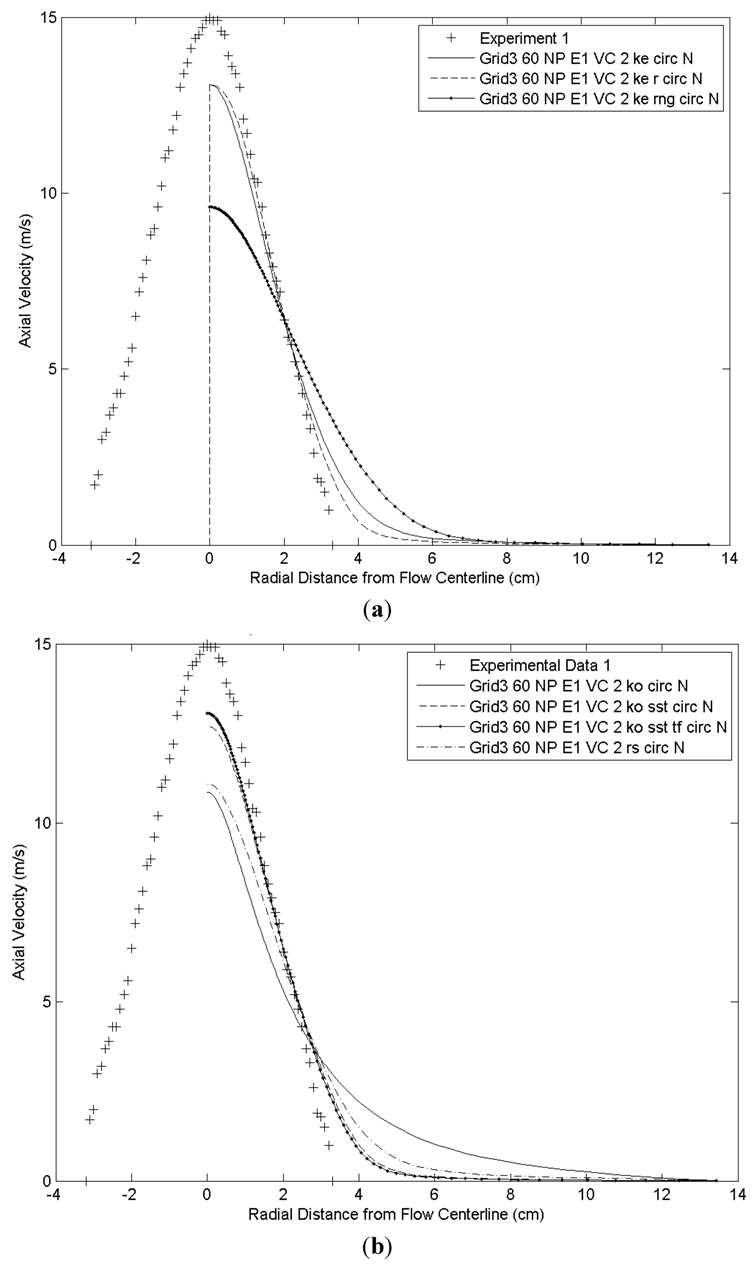
At 10 cm from the origin of the annular air jet, the k-ε models show larger variations than the k-ω models and produce both the best and the worst match. The k-ε realizable model most closely predicts the experimental results, to within 6% at the jet axis, while the RNG k-ε model produces the worst results, with an error of more than 30% at the jet axis. The standard k-ε model and all of the k-ω models fall in between these two results. The Reynolds stress model produced results similar to all the k-ω models and to the standard k-ε model.
At 20 cm the realizable k-ε model still yields results that agree best with experiment. The standard k-ε model performs nearly as well, having a broader velocity profile at its tail end. The RNG k-ε model predicts the profile poorly, similar to its results at the upstream cross section.
The results of the k-ω family of models at 20 cm distance were found to be similar to those at 10 cm. The agreement with experiment was improved by including the shear stress transport (sst) option and further improved by including the transitional flow (tf) option. The Reynolds stress model yielded poor results once again. Overall, the differences between the results are greater at 20 cm distance. Overall, the realizable k-ε and the k-ω sst tf models gave best results. All the models predict a faster decay of the centerline velocity at 10 cm and 20 cm, demonstrated in the graphs by the lower peak of the velocity profiles, compared to experiment. This behavior is due to the well-known tendency of RANS models to over predict mixing.
4. Discussion
The experimental data gathered from the flow field created by this coaxial jet with staggered nozzles, together with the results from the
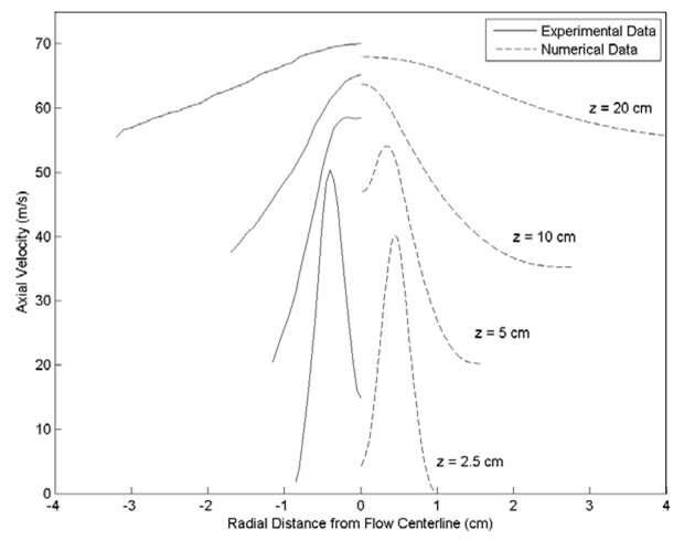
k-ε realizable model simulations are examined here more fully. The overall velocity field pattern is summarized here by the compound velocity profile graph in
Figure 19 which shows the experimental data for Experiment 1 and the corresponding numerical data extracted from a simulation using Grid4_NP_E1 and the
k-ε realizable model. This graph also shows the plateau in the plot of the axial velocity
vs. radius at
z = 5 cm. A similar plateau occurs in the same plot for the numerical results at
z = 8 cm. The numerical centerline velocity at
z = 8.5 cm agrees well with the experimental centerline velocity at
z = 10 cm. The under prediction of the mixing of the two jets by the
k-ε realizable model upstream of
z = 8 cm is once again shown. In contrast, further downstream, this turbulence model over predicts mixing, causing the centerline velocity to decrease faster than in reality. Why this model shows such inconsistent mixing is not known, but is deserving of study.
Ko and Kwan [
5] and Ribeiro and Whitelaw [
7] found that the turbulence intensity is greatest in the mixing layers formed as the two jets merge.
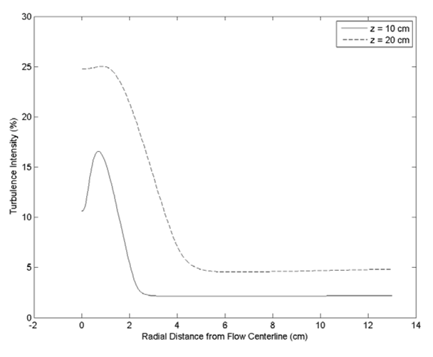
Figure 20 shows the numerical turbulence intensity for Experiment 1 at 10 cm and 20 cm from the cap face. It is noteworthy that at 10 cm from the cap face, even though the axial velocity profile shows the jets have fully merged, the variation in turbulence intensity shows that the velocity difference between the two jets created an annulus of high turbulence intensity. At 20 cm from the cap face, this annulus no longer exists due to turbulent mixing. Each plot was calculated from the turbulent kinetic energy and the centerline velocity at each of the two distances from the cap face. Consequently, the higher turbulence intensity at
z = 20 cm compared to
z = 10 cm is due to the drop in centerline velocity and the slow dissipation of the turbulent kinetic energy in the flow between the two planes. Plots of the turbulence intensity in the near field were not made because of the marked difference between the experimental and numerical results in this region. Experimental measurement of the turbulence intensity throughout the flow field would be a valuable addition to the understanding of the jet created by this new nozzle design.
Figure 19.
Experiment 1: Comparison of offset experimental and numerical axial velocity profiles at 2.5 cm, 5 cm, 10 cm and 20 cm from the annular air nozzle.
Figure 19.
Experiment 1: Comparison of offset experimental and numerical axial velocity profiles at 2.5 cm, 5 cm, 10 cm and 20 cm from the annular air nozzle.
Figure 20.
Experiment 1: The numerical turbulence intensity at 10 cm and 20 cm from the cap face found using the coarsest Grid 3 and the k-ε realizable turbulence model.
Figure 20.
Experiment 1: The numerical turbulence intensity at 10 cm and 20 cm from the cap face found using the coarsest Grid 3 and the k-ε realizable turbulence model.
Table 4 shows the volume flow rate for all three experiments, found from the numerical models and from the experimental measurements of axial velocity. The nozzle flow rate is 0.14 m
3/min. Comparison of the values in
Table 4 with the nozzle flow rate shows that there has been a large amount of entrainment and that, as expected, it increases with distance from the gun head. Examination of the experimentally found flow rates shows that at all but the last cross section at
z = 20 cm, the entrainment increases moderately with velocity ratio, except between Experiments 2 and 3 at
z = 5 cm where it remains the same. At
z = 20 cm there is very little difference in the amount of entrainment between the three experiments possibly because of the qualitative similarity of the axial velocity profiles from about 5 cm onwards downstream. In all cases the numerical entrainment is greater than the experimental entrainment mainly because the numerical simulations predict a jet with a greater radius than actually occurs. These results were compared with those of Wall
et al. [
11]. The amount of entrainment found here is much higher than that found by Wall, but the nozzle geometry was very different, so any further comparison is of dubious value.
Table 4.
The experimental and numerical volume flow rate for all three experiments.
Table 4.
The experimental and numerical volume flow rate for all three experiments.
| Experiment | Entrainment at
z = 2.5 cm (m3/min) | Entrainment at
z = 5 cm (m3/min) | Entrainment at
z = 10 cm (m3/min) | Entrainment at
z = 20 cm (m3/min) |
|---|
| 1 | Experimental | 0.35 | 0.41 | 0.64 | 1.16 |
| Numerical | 0.43 | 0.56 | 0.82 | 1.49 |
| 2 | Experimental | 0.40 | 0.46 | 0.69 | 1.13 |
| Numerical | 0.45 | 0.59 | 0.87 | 1.62 |
| 3 | Experimental | 0.42 | 0.46 | 0.81 | 1.17 |
| Numerical | 0.47 | 0.62 | 0.92 | 1.72 |
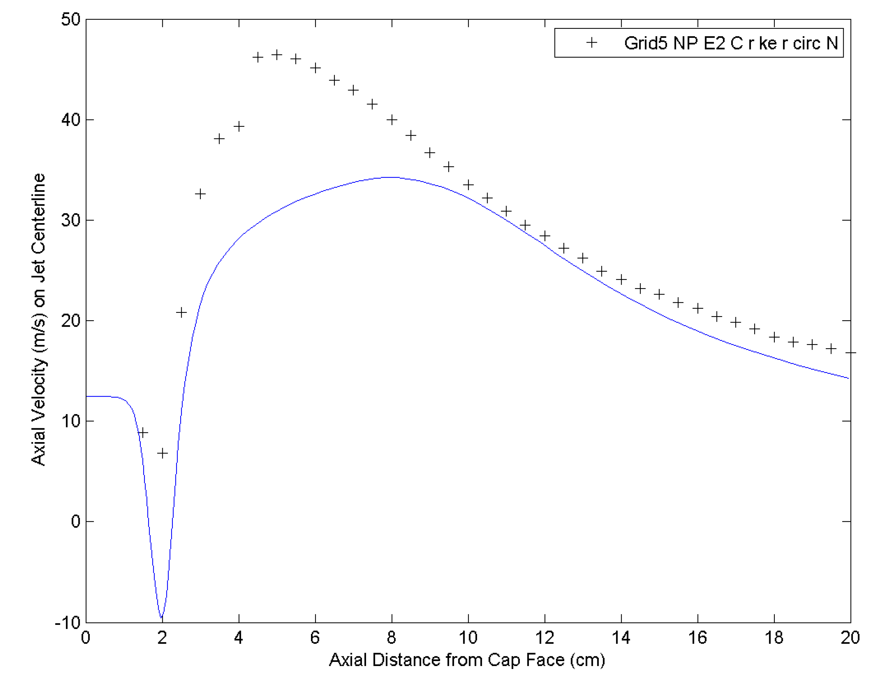
The comparison of the experimental and numerical axial velocity data along the centerline is shown in
Figure 21 and the comparison of the near field static pressures on the centerline is shown in
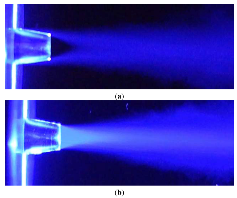
Figure 22. There is a striking qualitative difference at the position right after the two jets meet. The numerical results predict the presence of a small recirculation zone, extending between 2 mm and 6 mm downstream from the end of the central nozzle. The presence of the recirculation zone was never detected in the experiments. Indeed, the flow visualization shown in
Figure 9 confirmed that there was no recirculation zone in the experiments. The presence of a radially inward velocity component in the annular air jet velocity may prevent the formation of a recirculation zone when the ratio of the annular to axial jet velocity axial components would otherwise cause one. The presence of the recirculation zone in the numerical results leaves the cause of the broadening of the numerical simulation profiles, relative to the experiments, less clear cut than in the case of a single jet. It is important to note that all of the turbulence models predicted the recirculation zone, contrary to the experimental data. Thorough examination of the numerical results showed that none of the modeling variables, specifically the mesh density, turbulence model, boundary conditions, or discretization could have caused the numerical recirculation zone. Better understanding of the simulated flow field would include determining how much of the profile broadening at
z =10 cm in numerical simulations is due to higher diffusion calculated by the
k-ε realizable turbulence model, and how much is due to the presence of the non-physical recirculation zone upstream. This study was not intended to answer this question but the cause of the numerical recirculation zone needs to be studied in future work.
Figure 21.
Experiment 2: The Centerline Velocity: Comparison of numerical (line) and experimental (crosses) results.
Figure 21.
Experiment 2: The Centerline Velocity: Comparison of numerical (line) and experimental (crosses) results.
Figure 22.
Experiment 2: The Near Field Centerline Static Pressure: Comparison of numerical (line) and experimental (crosses) results.
Figure 22.
Experiment 2: The Near Field Centerline Static Pressure: Comparison of numerical (line) and experimental (crosses) results.
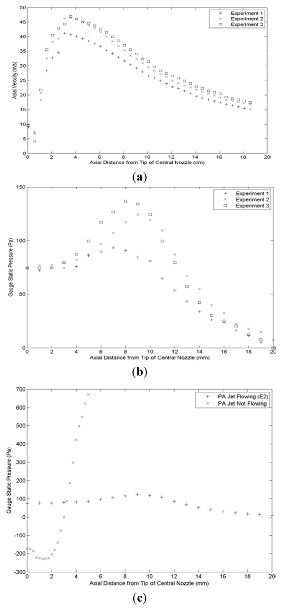
The positive gauge static pressure, recorded experimentally, but not predicted numerically, near the particle jet nozzle also deserves a full investigation. This positive gauge pressure was not expected. Chigier and Beer [
3] found that when the annular air jet is dominant, the gauge static pressure on the jet centerline in the near field is negative not positive. Ko and Kwan [
5] also found that the time averaged static pressure in the flow field of coaxial jets was not uniform. A likely explanation for this positive gauge pressure is the staggered design of the nozzle combined with the angling in of the annular air jet, directing it towards the jet axis. Another possible contributor is the difference in boundary conditions of the annular jet near field. On its inner side, this jet is bounded by the solid surface of the outside of the central jet nozzle. On its outer side, the annular air jet is free and able to entrain the surrounding atmosphere. The negative gauge static pressure found in the near field of the jet when the central jet is shut off is qualitatively consistent with the findings of Chigier and Beer [
3] for the case of no flow in the central jet.
Figure 19,
Figure 21 and
Figure 22 show the strongest discrepancy between the experimental and numerical results is in the jet merging zone. Judging by the numerical results the two jets merged at
z = 9 cm. At that location the velocity profile had a single peak and the centerline velocity profile shows its maximum. The experimental results, however, show that the two jets merged at approximately
z = 5 cm. This discrepancy is certainly affected by the presence of the recirculation zone. The downstream locations, after
z = 10 cm show a good match between numerical and experimental values, although the difference between the two results slowly increases with distance from the gun head.
The results of all simulations using two equation RANS models do not compare satisfactorily with the experimental data in the near field of the mixing zone. These differences are probably due to the reliance of these models on the Boussinesq hypothesis, their single point nature, and the largely empirical nature of the turbulent dissipation equation as pointed out by Shih
et al. [
12]. The Reynolds Stress model didn’t do any better, although it does not rely on the Boussinesq hypothesis. Hanjalic [
13] identified the limitations of the Reynolds stress model.
The
k-ε realizable model gave the best results in this flow probably due to an improved dissipation rate conservation/transport equation and the calculation of the eddy viscosity developed by Shih
et al. [
12]. They show that in all cases their changes to the standard
k-ε model provide results that are better than, or comparable to those of the original model. This work confirms that finding, at least for the coaxial jets being studied.
5. Conclusions
The numerical simulations modeled the concentric jet flow produced by this staggered nozzle with limited success in the near field, although the overall trends in the experimental data between the three experiments agreed with the overall trends in the numerical results. However, the limitations of all the RANs models in modeling isothermal coaxial jets need to be taken into account when modeling two phase flow and two phase flow with combustion.
Amongst all the two-equation models and the Reynolds stress model, the best results were obtained by the k-ε realizable model, closely followed by the k-ω sst tf model. However, all of the models predicted the existence of a recirculation bubble in all three cases, regardless of the jet momentum ratio. None of these flow regimes generated the recirculation bubble in the experimental work. The presence or absence of a toroidal shaped recirculation zone is important for the ultimate use of these results in flame deposition of a polymer powder coating. This recirculation zone will disrupt the smooth flow of the two-phase particle air stream even in the presence of flame.
The positive static pressure on the jet centerline in the jet near field was unexpected and shows the mixing in the near field created by this nozzle deserves further study. Future work must also include measurements of all components of the instantaneous velocity throughout the jet, including determination of the Reynolds stresses.


