Prediction of Ship Painting Man-Hours Based on Selective Ensemble Learning

Abstract

The precise prediction of painting man-hours is significant to ensure the efficient scheduling of shipyard production and maintain a stable production pace, which directly impacts shipbuilding cycles and costs. However, traditional forecasting methods suffer from issues such as low efficiency and poor accuracy. To solve this problem, this paper proposes a selective integrated learning model (ISA-SE) based on an improved simulated annealing algorithm to predict ship painting man-hours. Firstly, the improved particle swarm optimization (MPSO) algorithm and data grouping techniques are employed to achieve the optimal selection and hyperparameter optimization of base learners, constructing a candidate set of base learners. Subsequently, the simulated annealing algorithm is improved by adding random perturbations and using a parallel perturbation search mechanism to enhance the algorithm’s global search capability. Finally, an optimal set of base learners is composed of the candidate set utilizing the ISA-SE model, and a heterogeneous ensemble learning model is constructed with the optimal set of base learners to achieve the precise prediction of ship painting man-hours. The results indicate that the proposed ISA-SE model demonstrates improvements in accuracy, mean absolute error, and root mean square error compared to other models, validating the effectiveness and robustness of ISA-SE in predicting ship painting man-hours.

1. Introduction

Ship painting, as one of the three pillar processes of modern ship construction, runs through the entire shipbuilding process. Serving as a productive method for hull protection, it markedly mitigates the harmful impact of the ship’s demanding operational environment, curbing hull corrosion, cracking, and related issues. Beyond affording robust protection, painting operations also confer aesthetic enhancements, diminish resistance, and yield other ancillary benefits [1,2]. According to data from the China Shipbuilding Research Institute, the painting cost constitutes 8–10% of the total price for newly constructed ships in the domestic shipbuilding process. In advanced shipyards, such as those in Japan and South Korea, this proportion ranges from 5% to 6%, with specific shipyards even achieving percentages as low as 3% to 5%. In addition, as far as painting man-hours are concerned, some leading domestic shipbuilding companies consume three times as much as German shipyards did 15 years ago three times. Consequently, a considerable disparity exists between domestic painting costs and efficiency in comparison to developed countries, and addressing this gap is imperative to enhance painting efficiency and reducing costs. Man-hours, serving as a pivotal unit for cost measurement, constitute a crucial metric for the rational planning and scheduling of enterprise production. Rapid and precise estimation of painting man-hours stands as an effective strategy for elevating enterprises’ international competitiveness.

Within the realm of ship painting, numerous uncertainties arise from the interplay of personnel, processes, and environmental factors, rendering the prediction of man-hours a challenging endeavor. Typically, enterprises rely on process flow and historical experience to forecast man-hours; however, the accuracy of such predictions often needs to improve due to the multifaceted nature of the influencing factors. Consequently, the implementation of precise task assignments becomes a formidable challenge. Establishing a rational and efficient method for predicting painting man-hours holds the potential to intricately allocate a man-hour to each painting task. This, in turn, facilitates effective control over painting costs and production schedules, thereby enhancing the competitive edge of shipbuilding enterprises on the international stage.

The extensive application of machine learning and deep learning has proven effective not only in solving linear problems [3] but also in exhibiting superior predictive capabilities in handling nonlinear issues [4], coupled with a robust self-learning capacity [5]. Scholars, both domestically and internationally, have conducted predictive studies on man-hours across various industries, including mechanical and electrical engineering [6], as well as construction and building materials [7]. Minhoe Hur et al. [8] employed both the MLR (multiple linear regression) and CART (classification and regression trees) models, which balance model interpretability and accuracy for predicting shipbuilding man-hours. Their research demonstrated that the proposed models outperform traditional methods and expert predictions. Nur Najihah Abu Bakar et al. [9] proposed a data-driven approach based on cold ironing forecasting of ship berthing, which includes various models such as artificial neural networks, decision trees, etc., and the results show that the artificial neural network model can handle the complex nonlinear port activity prediction problem. The authors of [10] introduced a data-driven approach, combining multiple linear regression (MLR) with building information modeling (BIM) to establish a work-hour prediction model. The feasibility of this method was validated through its application in estimating labor man-hours in steel structure manufacturing. However, there are limitations to a single machine-learning model.

Ensemble learning, which combines a series of learners through certain rules to achieve a more significant generalization performance than individual learners [11], is categorized into homogeneous and heterogeneous ensembles [12]. Heterogeneous ensembles, in particular, have shown outstanding predictive effectiveness across various fields. Shuli Wen et al. [13] proposed a heterogeneous integration method for optimal time interval forecasting of solar power generation based on a stochastic ship motion model and verified the feasibility of the method on the power system of a large oil tanker, which provides a reliable reference for ship power system operators to realize better energy management. Zhou Sun et al. predicted ship fuel consumption by constructing a heterogeneous integrated learning model, which was experimentally verified to produce excellent prediction results. Zeyu Wang et al. [14] compared 57 heterogeneous ensemble learning models constructed from six base models using an exhaustive search method to identify the optimal model for predicting building energy consumption. Zhao Yuexu et al. [15] built a heterogeneous ensemble learning model from the perspectives of model, sample, and parameter diversity, aiming to predict the duration of traffic accidents. These studies indicate that constructing heterogeneous ensemble models can effectively improve prediction accuracy. However, these models often lack optimization of the hyperparameters of the base learners, potentially leading to suboptimal solutions and significant influence from the choice of base learner hyperparameters. To address this, Park Uyeo et al. [16] optimized the hyperparameters of base learners when constructing heterogeneous ensemble models, thereby enhancing the persuasiveness of their predictions. Chen Cheng et al. [17] proposed an integrated learning (EL) based unmanned surface vehicle dynamics model for accuracy prediction and used particle swarm optimization and genetic algorithm to optimize the hyperparameters of the base learner.

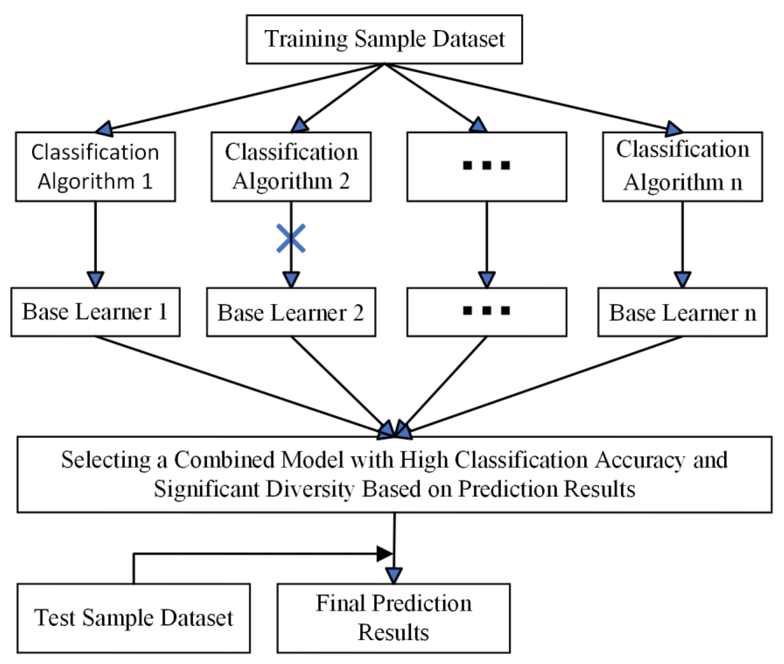
While ensemble learning has demonstrated outstanding predictive performance across various fields, the use of a large number of learners may lead to redundancy and longer computational times, potentially giving rise to issues such as overfitting and underfitting in prediction outcomes [18]. To address this challenge, selective ensemble learning has emerged [19]. The core idea behind selective ensemble learning is to select superior learners from a group of individual learners based on a specific strategy and then integrate them to form a more generalized classifier. Shuai Liu et al. [20] proposed a homogeneous selective ensemble forecasting framework based on an improved differential evolution algorithm to enhance the accuracy of hydrological forecasting. Huaiping Jin et al. [21] employed a soft measurement method based on data augmentation and selective ensemble for predicting measurement results, validating the effectiveness and excellence of this approach. Zhang Fan et al. [22] introduced a selective ensemble learning method based on the local model prediction accuracy and an adaptive weight calculation method for submodels. Simulations using accurate spatial dynamic wind power prediction data demonstrated the effectiveness of the proposed method in handling nonlinear, emotional, and multi-rate data regression problems in wind power generation. Additionally, Huaiping Jin et al. [23] proposed a selective ensemble model based on finite mixture Gaussian process regression for wind power prediction. The results outperformed traditional global and ensemble wind power prediction methods, effectively addressing the temporal changes in wind power data while maintaining high predictive accuracy. However, it is worth noting that the scholars mentioned above did not perform selection on the individual learners when constructing selective ensemble learning models. This oversight could directly impact the final predictive results.

The studies of the scholars mentioned above show that there are limitations of a single learner; in contrast, the generalization performance of integrated learning is higher, which is more suitable for research in complex contexts, and selective integrated learning optimizes the individual-based learners on the basis of integrated learning, which further optimizes the structure of the model and improves the performance of the model. However, in the above study, the selected individual-based learners were not analyzed for their compatibility with the research context, and the direct selection may lead to non-optimal results.

Despite the positive applications of machine learning and deep learning across various fields, ranging from single models to ensemble learning formed by combining multiple models, experts and scholars have consistently affirmed their outstanding performance in prediction. However, in the context of predicting ship painting man-hours, there is a relatively limited amount of reported research. Due to the multitude of uncertainties affecting ships during the painting process, leading to the instability of painting man-hours, reliance on a single predictive model is restrictive and results in a significant decline in accuracy. Therefore, employing multiple algorithmic models with distinct characteristics as base learners to construct a selective ensemble learning model for prediction holds the potential to enhance accuracy and robustness significantly.

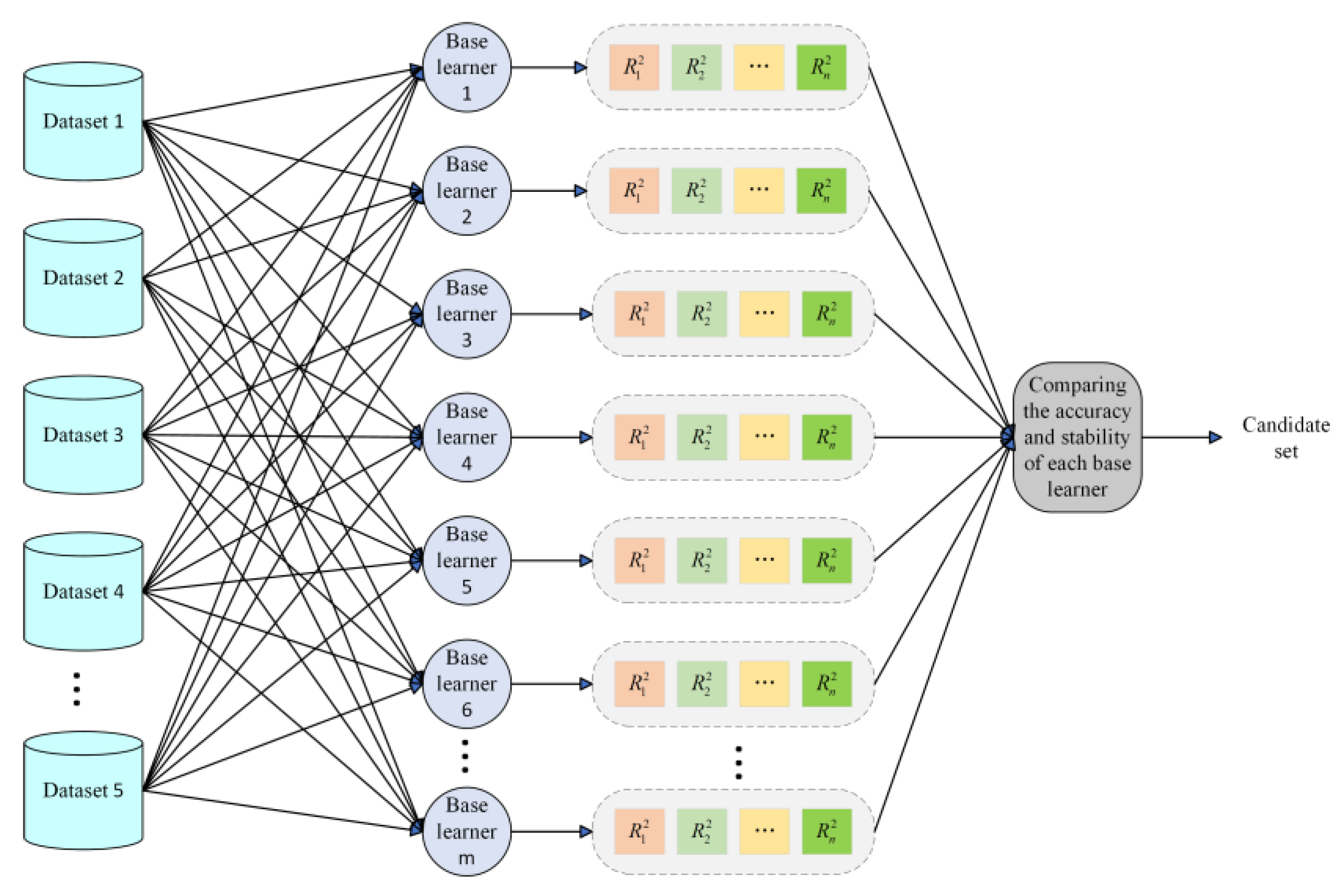
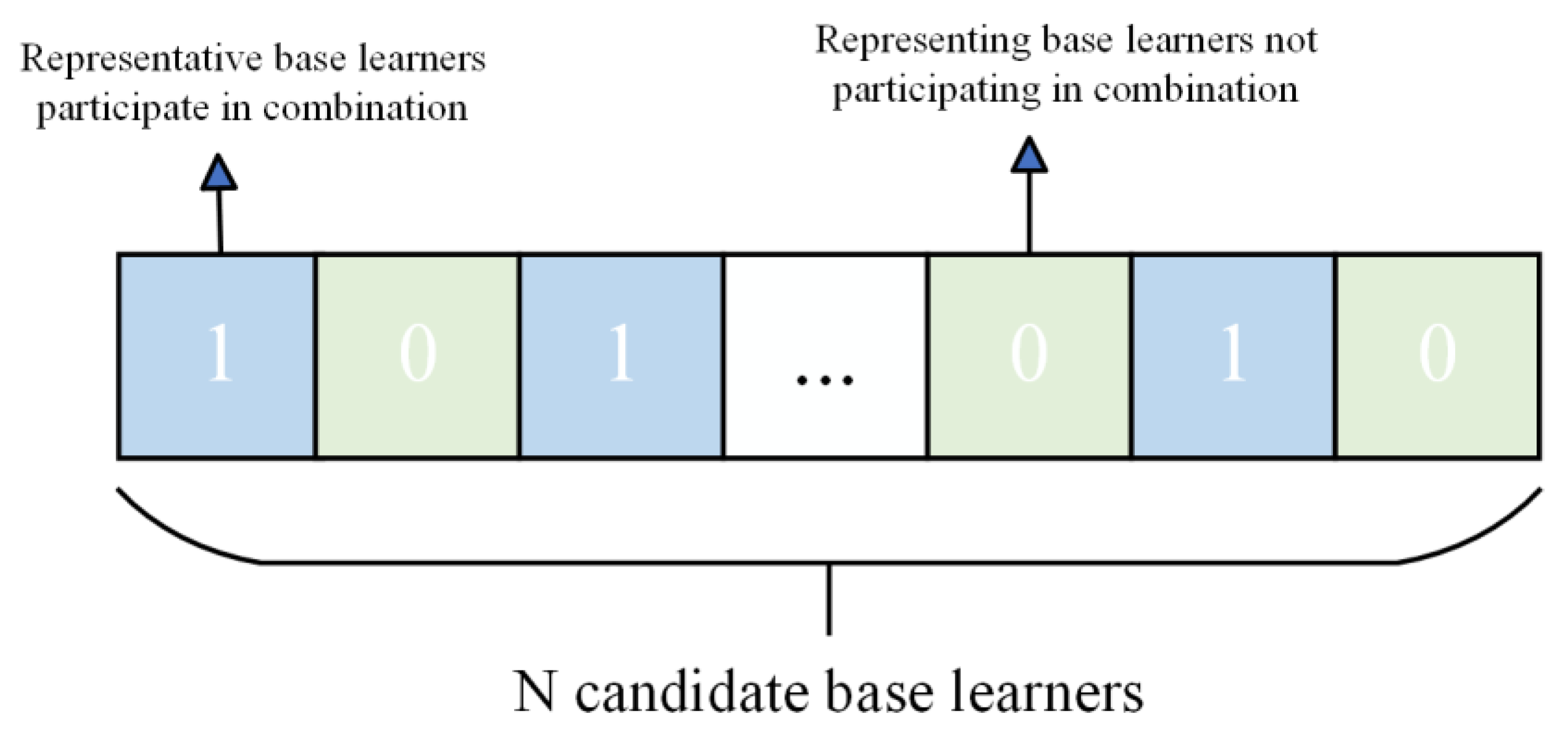
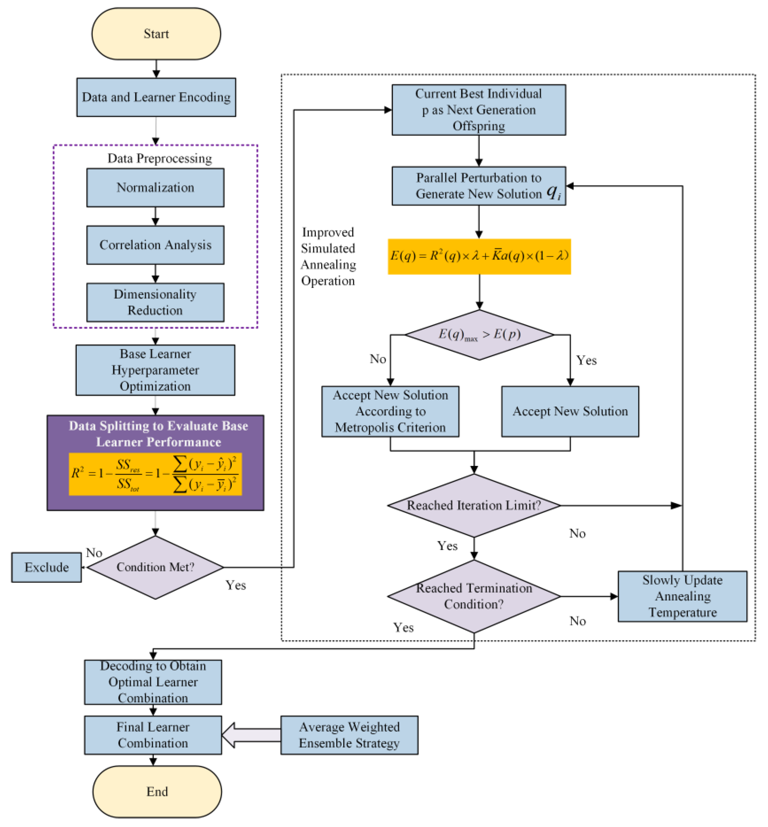
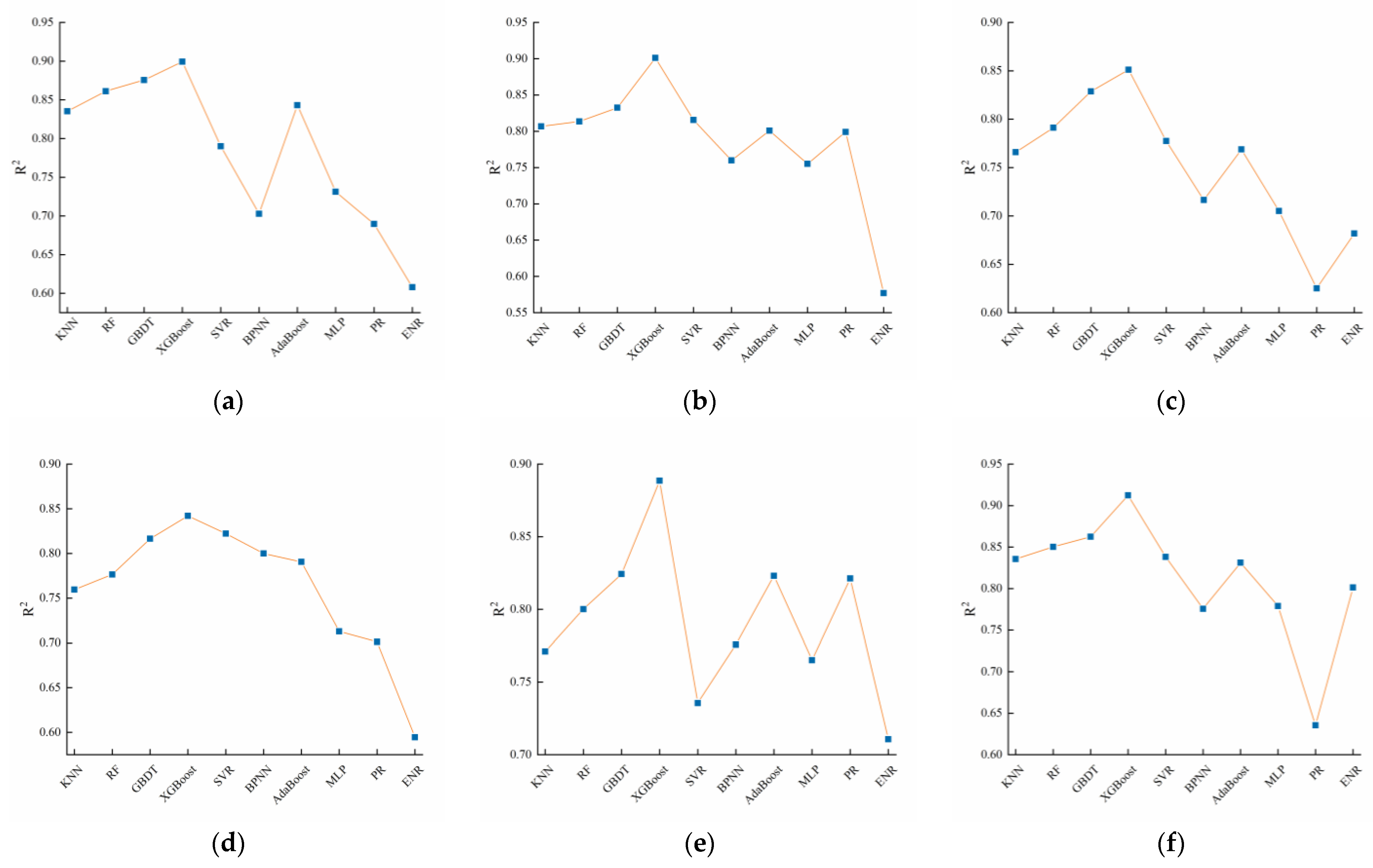
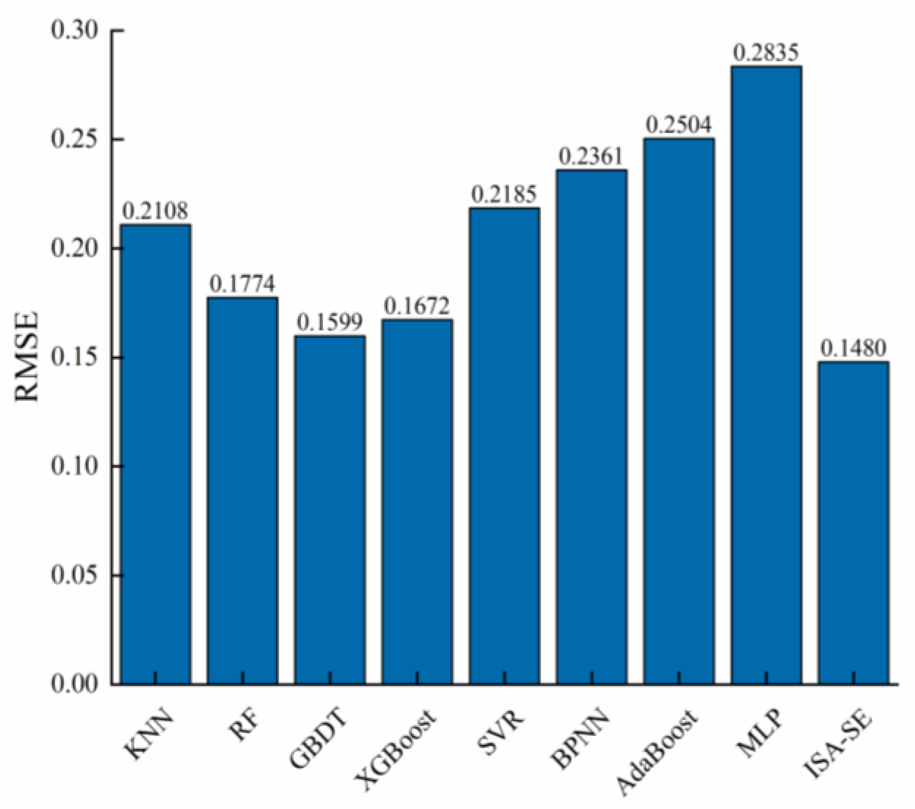
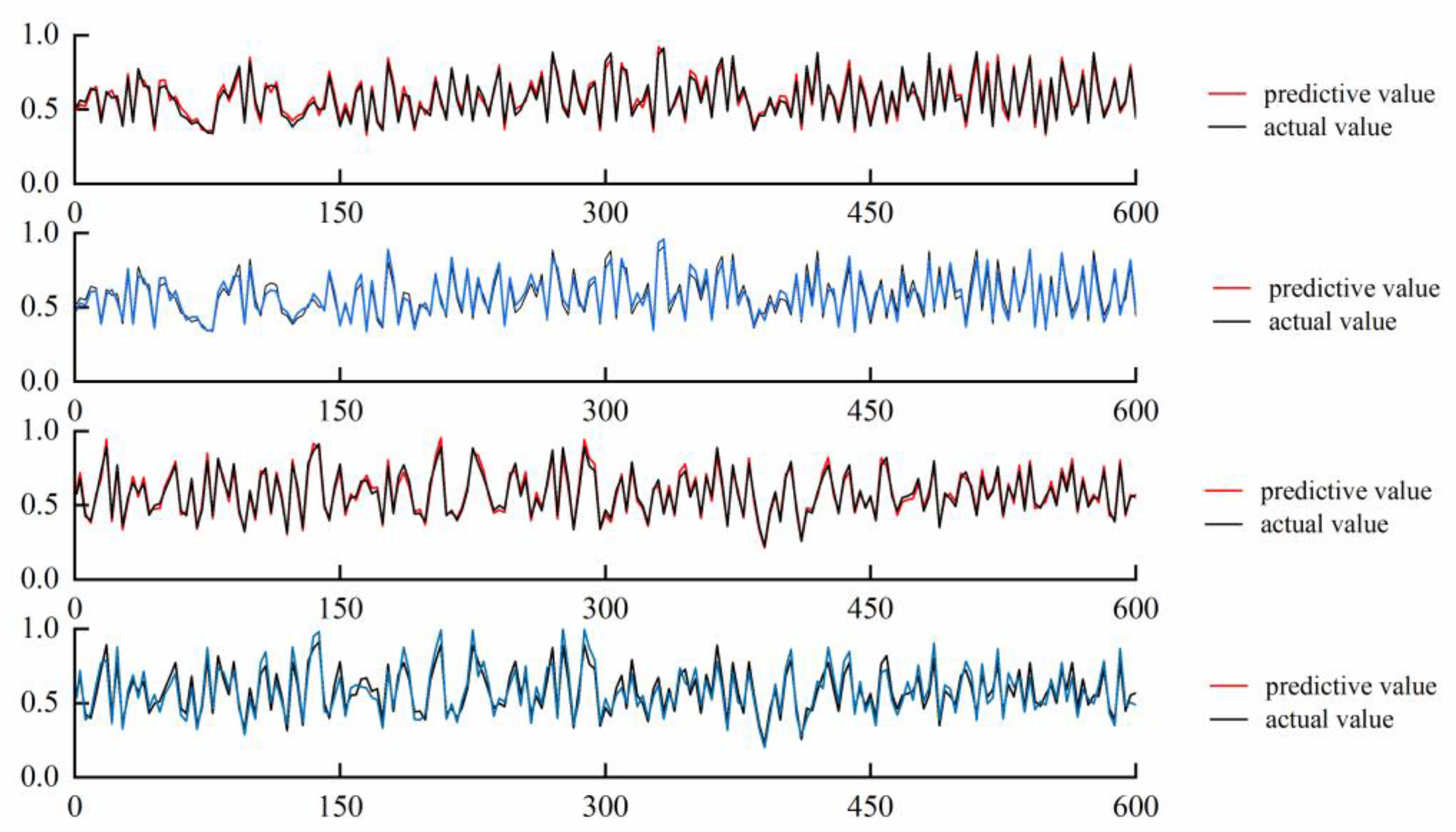
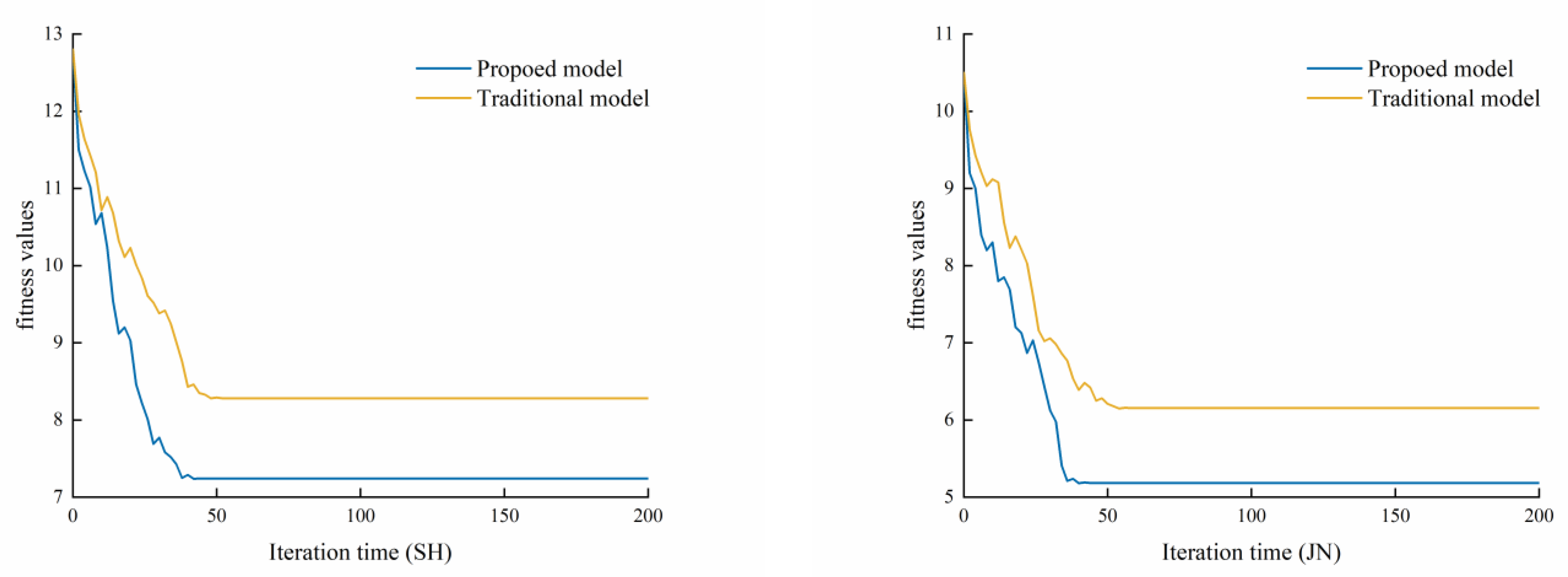
In view of the above shortcomings, this paper proposes a selective integrated learning model (ISA-SE) based on an improved simulated annealing algorithm to predict the man-hours of ship painting. This model employs ten different algorithms, including random forest (RF), support vector regression (SVR), and extreme gradient boosting (XGBoost), as base learners. Initially, the hyperparameters of these ten base learners are optimized through cross-validation and the MPSO algorithm. Subsequently, the dataset is randomly divided into six subsets using data grouping techniques. The optimal hyperparameters of the base learners are utilized as initial data, and predictions are made using each base learner separately. Base learners that meet the criteria are selected as candidate learners based on a comparison of the prediction results. To address the potential issue of local optima in the simulated annealing algorithm, a selection approach incorporating increased random perturbations is adopted, and a parallel perturbation search is conducted on this selection path to expand the search range. Finally, the improved simulated annealing algorithm is applied to further filter the candidate learners, selecting the optimal combination of diverse base learners to predict ship painting duration accurately.

2. Establishment of Selective Ensemble Learning Model

2.1. Selective Ensemble Learning

The core idea of selective ensemble learning is to select a representative subset of classifiers from numerous classifiers for combination, eliminate classifiers with poor classification performance and redundancy, and comprehensively improve the generalization performance and prediction efficiency of classifiers. The basic framework is shown in Figure 1.

2.2. Selective Integration Technology

In ensemble models, algorithms are often chosen based on experience. However, the predictive capabilities of models can vary in different contexts, making it challenging to guarantee prediction accuracy. Additionally, when combining basic algorithms, the multitude of combinations makes traditional exhaustive search methods time-consuming. Moreover, the complex structure of ensemble models makes it challenging for conventional mathematical methods to effectively and reasonably allocate weights. To address these issues, this paper proposes a selective ensemble learning model named ISA-SE, which includes four essential parts: the optimization of learner hyperparameters, selection of learner performance, improvement of the simulated annealing algorithm, and optimization of learner combinations.

2.2.1. Optimization of Learner Hyperparameters

In this study, ten base learners were selected based on the characteristics of the ship painting dataset, and the hyperparameters that significantly influence the performance of these learners were optimized. This optimization aims to identify the optimal parameter model within the specific context of this dataset. Common methods for hyperparameter tuning include manual adjustment [24], grid search [25], random search [26], and machine learning-based approaches [27,28]. Machine learning algorithms, through iterative processes, are adept at rapidly identifying the most effective combinations of parameters. In this research, an enhanced particle swarm optimization (MPSO) algorithm [29] was employed to determine the optimal parameters of the base learners, thus creating the MPSO-X model. MPSO incorporates mutation operations from genetic algorithms into the standard particle swarm framework to mitigate the issue of local optima. The process of tuning the hyperparameters, such as the error penalty factor C and the kernel function coefficient g for the base learner SVR, is illustrated in Figure 2. The hyperparameter optimization for other base learners is similarly conducted using this computational process.

2.2.2. Performance Screening of Learners

Utilizing data grouping techniques, the preprocessed dataset was randomly divided into subsets, which were then individually trained using the optimized models of the base learners. A comparative analysis of the training outcomes was conducted to evaluate the predictive precision of each base learner across different training sets. This involved calculating the overall mean accuracy of each learner across all training sets and comparing these means with the average predictive accuracies of other algorithmic models. Subsequently, the comparative results were systematically ranked, leading to the exclusion of models demonstrating considerable variance and subpar average predictive accuracy across diverse datasets. Figure 3 illustrates this methodology in detail.

In this study, the coefficient of determination, $R^2$, was adopted as the metric for evaluating predictive accuracy. The $R^2$ value ranges from 0 to 1, with values closer to 1 indicating a higher proportion of variance in the dependent variable ($y$) that is predictable from the independent variable ($x$). This denotes a closer alignment of the regression line to the observed data points. A higher $R^2$ value reflects a better fit of the model, implying that the variability in $x$ more effectively explains the variations in $y$, thereby signifying enhanced predictive accuracy.

The sum of squared residuals is:

$$S{S}_{res}={\displaystyle \sum (y_i}-{\widehat{y}}_i{)}^2$$

(1)

The total sum of squares is:

$$S{S}_{tot}={\displaystyle \sum }{(y_i-{\overline{y}}_i)}^2$$

(2)

The expression for $R^2$ is:

$$R^2=1-\frac{S{S}_{res}}{S{S}_{tot}}=1-\frac{{\displaystyle \sum (y_i}-{\widehat{y}}_i{)}^2}{{\displaystyle \sum }{(y_i-{\overline{y}}_i)}^2}$$

(3)

Among them, $y_i$ represents the true value, ${\widehat{y}}_i$ represents the predicted value, and ${\overline{y}}_i$ represents the sample mean.

The average accuracy of the algorithm model is:

$$D_X=\frac{1}{n}{\displaystyle \sum _{i=1}^n{R}_i^2}$$

(4)

Among them, $X$ represents the algorithm, $n$ represents the number of data groups, and $R_i^2$ represents the $R^2$-value of the i-th group of data.

2.3. Improved Simulated Annealing Algorithm

The simulated annealing algorithm [30,31,32], owing to its similarity to the annealing process in physics and combinatorial optimization problems, has found application in solving combinatorial optimization. Due to the complexity of combinatorial types, improving the simulated annealing algorithm can enhance its efficiency and accuracy. Consequently, following the optimization and selection process of base learners via the MPSO algorithm and data grouping techniques, an improved simulated annealing algorithm, in conjunction with an average weighting method, is employed. This approach selects the optimal set of base learners from the candidate pool, constructing a heterogeneous ensemble learning model. This model is adept at achieving accurate predictions of the man-hour required for ship painting.

In the process of optimizing combinations of candidate learners using the simulated annealing algorithm, random perturbations can potentially lead to local optima. To avoid this situation, we increase the disturbance path from one to three during random perturbation, and during this process, three disturbance paths are generated simultaneously to obtain three new solutions. We compare the three new solutions and select the optimal one, which expands the search range. Additionally, during the optimization of combinations using the improved simulated annealing algorithm, there is a possibility of redundancy with certain types of learners or multiple learners of the same type being present in the combination, which could diminish the generalization capability of the learner ensemble. To avoid this, we redefine the integration accuracy $E(q)$ for generating new solutions under the Metropolis criterion by introducing the $R^2$ and $Kappa$ coefficients and using $\lambda$ to regulate the weights to ensure that the new solutions generated guarantee the prediction accuracy along with the variability of the base learner. The redefined formula for $E(q)$ is as follows:

$$E(q)=R^2(q)\times \lambda +\overline{K}a(q)\times (1-\lambda )$$

(5)

where $q$ is the new solution (base learner combination) screened during each iteration, $R^2$ is used to evaluate the performance of the combination, $\overline{K}a$ denotes the average value of $Kappa$ coefficients, $\lambda$ is used to regulate the weight of the evaluation metrics $R^2$ and $\overline{K}a$ in the metric $E(q)$, and when $\lambda$ is bigger, $R^2$ plays a greater role, and when $\lambda$ is smaller, $Kappa$ coefficients $\overline{K}a$ plays a greater role. the expression of $\overline{K}a$ is given by:

$$\overline{K}a=\frac{1}{n}{\displaystyle \sum _{i=1}^{n}K{a}_i}$$

(6)

where $K{a}_i$ denotes the $Kappa$ coefficients of the two base learners in the i-th group.

The $Kappa$ coefficient takes values in the range of [–1, 1], when the $Kappa$ coefficient is closer to −1, it indicates that the prediction variability of the learner is greater; the closer it is to 1, the result is the opposite. The coefficient is calculated by the formula:

$$Ka=\frac{{\phi }_1-{\phi }_2}{1-{\phi }_2}$$

(7)

where ${\phi }_1$ and ${\phi }_2$ are the probabilities of agreement and disagreement between the two learners, respectively. The formula is:

$${\phi }_1=\frac{a+d}{m}$$

(8)

$${\phi }_2=\frac{(a+b)(a+c)+(c+d)(b+d)}{m^2}$$

(9)

where $a(d)$ denotes the number of samples predicted correctly (incorrectly) by both learners, $b(c)$ denotes the number of samples with one correct and one incorrect, and m is the total number of samples.

Table 1. Combination of the prediction results of the two learners.

	$h_{i}correct$	$h_{i}incorrect$
$h_{j}correct$	$a$	$c$
$h_{j}incorrect$	$b$	$d$

gives the combination of two different learners $h_i$ and $h_j$$\left(i,j=1,2,\cdots ,N,i\ne j\right)$ on the prediction results.

$$a+b+c+d=m$$

(10)

The improved simulated annealing algorithm is utilized to randomly initialize and select learners from the set of candidate base learners. To ascertain whether each learner participates in the ensemble, a binary representation is employed, where ‘1’ signifies the selection and ‘0’ indicates the exclusion of a particular learner from the candidate set. This selection process is visually represented in the encoding structure, as illustrated in Figure 4. The procedure for selecting learners based on the improved simulated annealing algorithm is systematically detailed in Algorithm 1.

Algorithm 1. Improved Selective Integration Algorithm for Simulated Annealing

Input: set of candidate learners $N=\{n_1,n_2,n_3\dots .n_n\}$ Output: set of base learners $M=\{m_1,m_2,m_3\dots m_m\}$ Step 1: Initialize the temperature $t>0$, generate the initial solution $p=\{1,0,0\dots 1\}$ from the candidate set $N$ and compute the integration accuracy of $p$ as $E(p)$; Step 2: (1) Remove one or two learners with poor prediction results from the set of $p$; (2) Add one or two new learners to the set of $p$; (3) Remove one or two learners with poor predictions from the set of p and add one or two new learners. Using parallel perturbation, three new solutions $q_i$($i=1,2,3$) are randomly generated according to a certain probability, and $E(q_i)$ is the integration accuracy of the new solution $q_i$ achieved by the metric; Step 3: Compare to obtain the maximum value $E{(q)}_{\max }$ of $E(q_i)$ and judge whether to accept it or not based on the Metropolis criterion; Step 4: A solution stabilized at temperature t is obtained by continuous iteration. Assuming that the number of times a new solution is accepted at a certain temperature exceeds a set threshold, the temperature decreases more; Step 5: If the termination condition is met, the algorithm will be terminated and will be used as the final integrated set of classifiers, otherwise it will jump to Step 2; Step 6: Update the temperature t, according to the given temperature control function and jump to Step 2;

Metropolis guidelines for:

$$P=\left\{\begin{array}{r}\hfill 1,E{(q)}_{\max }>E(p)\\ \hfill e^{\frac{-(E{(q)}_{\max }-E(p))}{\lambda t}},E{(q)}_{\max }\le E(p)\end{array}\right.$$

(11)

where $t$ denotes the temperature and $\lambda$ denotes the scaling factor of temperature decrease. $P$ denotes the probability of accepting the new solution, when $E{(q)}_{\max }>E(p)$, it means that the accuracy of the new solution is higher than that of the solution in the previous state and the probability of accepting the new solution is 1. When $E{(q)}_{\max }\le E(p)$, it means that the accuracy of the new solution is lower than or equal to that of the solution in the previous state and the probability of accepting the new solution is $e^{\frac{-(E{(q)}_{\max }-E(p))}{\lambda t}}$.

2.4. Selective Integration Technology Forecasting Framework

Based on selective integrated learning to realize the prediction of ship painting man-hours, the calculation flow is shown in Figure 5.

The specific steps are as follows:

Step 1: Firstly, the data related to the influence factors of ship painting man-hours are preprocessed, and the hyper-parameters of the selected 10 base learners are optimized by five-fold cross-validation combined with the MPSO algorithm, respectively, and the optimal hyper-parameters are used as the initial parameters of these 10 base learners;

Step 2: Divide the dataset into six parts by data grouping technique, then train 10 base learners, respectively, analyze the output results of each learner, and keep the learners with high stability and evaluation index value over 0.7 to constitute the candidate base learners. At the same time, the base learners that do not meet the requirements are eliminated;

Step 3: The simulated annealing algorithm is improved, and the combination of candidate base learners is optimized using the improved simulated annealing algorithm, which is validated by the three evaluation metrics of MAE, RMSE, and accuracy, and the combinations of base learners with high variability and high accuracy are filtered out;

Step 4: The test set data are input into a combination of learners, and the outputs of each learner in the combination are used to predict ship painting hours by the average weighting method. The proposed method is compared with the ISA-SE model and the selective integrated learning model composed of the traditional simulated annealing algorithm to verify the effectiveness of the proposed method in predicting ship painting hours.

3. Ship Painting Man-Hour Model Analysis and Modeling

3.1. Data Pre-Processing

3.1.1. Data Acquisition and Characterization

According to the ship coating and painting technology and shipyard research, it is understood that in the process of ship construction, painting not only includes coating operations, but also includes surface pretreatment and secondary descaling activities before coating. Due to the special characteristics of the shipbuilding process, there are some painting operations in each stage of ship construction, and the painting operations are distributed in all stages of the ship construction process. The ship painting stage includes: raw material shot blasting pretreatment, workshop primer painting, and in-dock painting before section/stage/wharf/delivery. Ship painting man-hours are the times that should be spent to complete the painting work according to the specified process.

The ship painting process represents a highly complex and time-intensive operation. The efficiency of painting is influenced by a multitude of factors, leading to significant uncertainties in the time required for completion. Predominant factors impacting the duration include operator skill, working environment, production processes, equipment, and raw materials. Drawing on this theory and combining with the shipyard database and ship painting manuals, this study classifies the factors that mainly affect the painting man-hour, such as worker age, technical level, steel surface cleanliness, spraying methods, film thickness, coating area, segmental structure, temperature, humidity, and wind force, into four categories, namely, human factors attributes, process attributes, equipment and material attributes, and environmental attributes, and uses these factors as inputs to verify the feasibility of the ISA-SE-based ship painting man-hour prediction model proposed in this paper. The specific categories of factors influencing ship painting duration are delineated in

Table 2. Variables and classifications.

Attributes	Factor	Datatype
Human attributes	Age	Continuous variable
	Technical level	Ordinal categorical variable
Equipment and material attributes	Steel surface cleanliness	Ordinal categorical variable
	Spraying methods	Nominal categorical variable
Process attributes	Film thickness	Continuous variable
	Coating area	Continuous variable
	Segmental structure	Nominal categorical variable
Environmental attributes	Temperature	Continuous variable
	Humidity	Continuous variable
	Wind force	Continuous variable

. Based on these factors affecting man-hours, we selected painting data from container ships of two domestic shipbuilding companies. From each company’s database, 600 sets of comprehensive data were randomly selected for experimental purposes, hereafter referred to as the SH and JN datasets.

Given the complexity and intricacy of the influencing factors, our approach initially involves simplifying the model complexity. To this end, we employ Pearson’s correlation coefficient for a comprehensive correlational analysis aimed at identifying the key influencing factors. Subsequently, principal component analysis (PCA) is utilized to perform dimensionality reduction on the retained original data. This methodological strategy effectively streamlines the dataset, ensuring a more focused and efficient analysis while preserving the essential characteristics of the data relevant to the study’s objectives.

3.1.2. Data Encoding and Normalization

Prior to embarking on correlation analysis and dimensionality reduction, it is imperative to convert all variables into numerical data. Quantifiable variables, such as age, coating area, and film thickness, are straightforwardly represented through their numerical values. However, categorical variables like technical level and surface cleanliness necessitate the assignment of specific numerical encodings to facilitate their transformation into quantifiable data. The detailed methodology for this variable conversion process is systematically outlined in

Table 3. Variable conversion table.

Factor	Form	Conversion Value
Technical level	Junior worker	1
	Intermediate worker	2
	Senior worker	3
	Technician	4
	Senior technician	5
Steel surface cleanliness	Sa2	1
	Sa2.5	2
	Sa3	3
Segmental structure	A	1
	B	2
	C	3
	D	4
	E	5
	F	6
	G	7
Spraying methods	Brush coating method	1
	Roller coating method	2
	Air spray coating	3
	Airless spray coating	4

, ensuring a standardized approach for data preprocessing.

The normalization of features is imperative to mitigate the impact of differing scales among features and ensure comparability across various indicators. Standard normalization techniques include linear function normalization and zero-mean normalization. Linear function normalization involves a linear transformation of the raw data, mapping the results to a [0, 1] range, thereby achieving proportional scaling of the original data. The specific formula for this normalization process is as follows:

$$x_i=\frac{X_i-X_{\min }}{X_{\max }-X_{\min }}$$

(12)

In the normalization process, $x_i$ represents the normalized value of $X_i$, where $X_{\max }$ and $X_{\min }$ denote the maximum and minimum values of the dataset, respectively.

3.1.3. Selection of Variables

In the context of assessing the linear correlation between two variables, $X$ and $Y$, the coefficient of Pearson serves as a crucial statistical tool. For preprocessed data related to ship painting man-hours, one can employ Python code to analyze the correlation between various influencing factors and man-hours using the coefficient of Pearson. This analysis facilitates the categorization of correlations based on the coefficient magnitude. Using a coefficient of Pearson with an absolute value greater than 0.8 indicates a strong correlation between the variables. Values between 0.5 and 0.8 suggest a moderate correlation, while those ranging from 0.3 to 0.5 denote a weak correlation. Coefficients below 0.3 imply negligible or no correlation. The specific formula for calculating the coefficient of Pearson is as follows:

$$r=\frac{{\displaystyle \sum _{i=1}^n(X_i-\overline{X})(Y_i-\overline{Y})}}{\sqrt{{\displaystyle \sum _{i=1}^n{(X_i-\overline{X})}^2}}\sqrt{{\displaystyle \sum _{i=1}^n{(Y_i-\overline{Y})}^2}}}$$

(13)

Here, $r$ represents the coefficient of Pearson between $X$ and $Y$, $X_i$ and $Y_i$ are the individual sample points, and $\overline{X}$ and $\overline{Y}$ are the means of $X$ and $Y$, respectively.

According to the coefficient of Pearson, correlation analysis on a dataset comprising 1200 groups, the findings are comprehensively illustrated in Figure 6.

The bivariate Pearson’s test results elucidate the varying degrees of correlation between multiple factors and ship painting man-hours. Coating area and film thickness are highly correlated with painting man-hours. The technical level, steel surface cleanliness, spraying method, and segmental structure exhibit a moderate correlation. Age and temperature are weakly correlated with painting man-hours, while wind force and humidity have almost no correlation. Among these factors, there is a moderate correlation between age and technical level, but the correlation between other factors is relatively low, avoiding the issue of feature redundancy. Consequently, age, technical level, film thickness, coating area, steel surface cleanliness, temperature, spraying method, and segmental structure are selected as the eight primary features for predicting painting man-hours. However, using all eight features as inputs in the predictive model could potentially lead to an explosion in dimensionality, thereby increasing the variance in test data error. Therefore, simplifying the model is a crucial step in reducing variance, and dimensionality reduction is an effective strategy to address the problem of high dimensionality.

The principal component analysis (PCA) method employs a dimensionality reduction approach, projecting the original data into a few directions with maximum variance. This multivariate statistical analysis technique transforms multiple indicators into a smaller number of composite indices through orthogonal rotation. By applying the PCA algorithm for linear dimensionality reduction and determining the number of principal components based on the cumulative variance contribution rate, the model can be further simplified. This simplification not only enhances the efficiency of the model but also improves its generalizability.

The specific operations of the PCA algorithm are: (1) collecting p-dimensional random vectors and constructing a sample matrix; (2) calculating the eigenvector of the covariance matrix $\sum$ as ${\lambda }_1>{\lambda }_2>\cdot \cdot \cdot >{\lambda }_p$, and the corresponding unit eigenvector is $U_1,U_2,\cdot \cdot \cdot ,U_P$, where the transformation matrix is $A=U^{\prime }$, that is, the i-th row of $A$ is the unit eigenvector $u_i$ corresponding to the i-th characteristic root of $\sum$, and the variance of the i-th principal component $z_i$ is equal to the i-th characteristic root ${\lambda }_i$ of $\sum$; (3) preserving the principal components corresponding to cumulative variance contribution rate exceeding 90% and use them as input features for subsequent datasets.

The formula for the variance contribution rate of the k-th principal component $z_k$ is:

$${\eta }_k=\frac{{\lambda }_k}{{\displaystyle \sum _{k=1}^p{\lambda }_k}}$$

(14)

Theorem-type environments (including propositions, lemmas, corollaries, etc.) can be formatted as follows:

If $m$ principal components are taken, the cumulative contribution rate formula of principal components $z_1,z_2,\cdot \cdot \cdot ,z_m$ is:

$${\zeta }_m=\frac{{\displaystyle \sum _{k=1}^m{\lambda }_k}}{{\displaystyle \sum _{k=1}^p{\lambda }_k}}$$

(15)

In this study, a dataset comprising 1200 samples was employed, with a division of 900 samples for the training set and 300 for the testing set. PCA was applied to the training data for dimensionality reduction. The feature values and the corresponding variance contribution rates were calculated according to the previously described formulae, as detailed in

Table 4. Eigenvalues and variance contribution rate.

No.	Eigenvalue	Variance Contribution Rate/%	Cumulative Variance Contribution Rate/%
1	14.27	51.02	41.02
2	5.8	23.58	74.60
3	4.23	17.31	91.91
4	0.58	5.59	97.50
5	0.43	1.28	98.78
…	…	…	…
n	0	0	100

.

As shown in the table above, the cumulative contribution rate of the eigenvalues of the first three principal components reaches 90%, so three components are selected to replace the original variables. The standardized orthogonal rotation method was used to obtain the factor loadings of each factor on different principal components, and the resulting component matrices are shown in

Table 5. Composition matrix.

Data Item	Principal Component
	Component 1	Component 2	Component 3
Age	0.328	−0.597	0.553
Technical level	0.413	0.298	−0.335
Film thickness	0.732	−0.445	0.012
Coating area	−0.687	0.713	0.225
Steel surface cleanliness	−0.566	0.312	−0.679
Temperature	0.132	−0.377	0.028
Spraying method	0.435	−0.233	0.606
Segmental structure	−0.332	0.053	−0.258

.

The main component values obtained based on PCA dimensionality reduction technology are shown in the following formula:

$$\left\{\begin{array}{c}{z}_1=0.328x_1+0.413x_2+0.732x_3-0.687x_4-0.566x_5+0.132x_6+0.435x_7-0.332x_8\\ z_2=-0.597x_1+0.298x_2-0.445x_3+0.713x_4+0.312x_5-0.377x_6-0.233x_7+0.053x_8\\ z_3=0.553x_1-0.335x_2+0.012x_3+0.225x_4-0.679x_5+0.028x_6+0.606x_7-0.258x_8\end{array}\right.$$

(16)

In the formula, $x_1\dots x_8$, respectively, represent age, technical level, film thickness, coating area, steel surface cleanliness, temperature, spraying method, and segmental structure.

3.2. Basic Learner Parameter Settings

The selection of base learners for the ship painting process was determined based on the specific conditions of ship painting. In the practical ship spray painting process, the data storage for factors affecting painting man-hours is limited, and the prediction process involves nonlinear mapping. Consequently, considering the characteristics of ship painting man-hours and the strengths and weaknesses of various machine learning algorithms, ten suitable base learner models were identified. These models were then optimized for their principal hyperparameters using the modified particle swarm optimization (MPSO) algorithm, as described in Section 2.2.1. The optimization results are presented in

Table 6. Algorithm parameter settings.

Algorithm	Advantages	Optimization Parameters	Value
K-nearest neighbors (KNN)	Robustness	Number of neighbors, Minkowski distance	5, 2
Random forest (RF)	Fast training speed, simple computation	Number of trees, minimum samples in leaf nodes	100, 4
Gradient boosting decision tree (GBDT)	Effectively improves accuracy and efficiency in low-dimensional data	Number of trees, learning rate, subsampling ratio	100, 0.1, 0.6
Extreme gradient boosting (XGBoost)	Effectively prevents overfitting of recognition models	Step size, maximum depth of trees	0.2, 5
Support vector regression (SVR)	Suitable for small sample data	Penalty factor for misclassifications, kernel function coefficient	1.0, 0.001
Back propagation neural network (BPNN)	Achieves nonlinear mapping of input and output	Hidden layers, neurons in hidden layers	1, 4
Adaptive boosting (AdaBoost)	No need for feature selection, no overfitting	Number of trees, learning rate	100, 0.1
Multilayer perceptron (MLP)	Learn complex relationships Between features and targets through activation functions in each layer	Hidden layers, neurons in hidden layers	1, 4
Polynomial regression (PR)	Fast performance of linear methods, adaptable to a wide range of data	Polynomial degree, whether to fit intercept	3, False
Elastic net regression (ENR)	Handle predictions with multiple features and another feature using L1 and L2 regularization rules	Penalty coefficient, weight of L1 regularization	1.0, 0.5

.

3.3. Evaluation Indicators

To assess the efficacy of the proposed selective ensemble learning model in predicting ship painting man-hour, three evaluation metrics are employed: accuracy, mean absolute error (MAE), and root mean square error (RMSE). These metrics provide a comprehensive evaluation of the model’s performance, with accuracy indicating the overall correctness of the predictions, MAE reflecting the average magnitude of the errors in the predictions, and RMSE offering a measure of the square root of the average squared differences between the predicted and actual values. The utilization of these diverse metrics ensures a robust and thorough evaluation of the model’s predictive capabilities in the context of ship painting man-hour estimation.

The accuracy is a measure representing the proportion of correctly predicted samples out of all samples. It includes both correctly predicted positive and negative samples. The formula for calculating accuracy is as follows:

$$Accuracy=\frac{TP+TN}{TP+FN+FP+TN}$$

(17)

TP (true positives) are the correctly predicted positive observations; TN (true negatives) are the correctly predicted negative observations; FP (false positives) are the wrongly predicted positive observations; FN (false negatives) are the wrongly predicted negative observations.

MAE is used to measure the average absolute error between predicted values and true values. A smaller MAE indicates a better model, and its definition is as follows:

$$MAE=\frac{1}{\mathrm{n}}{\displaystyle \sum _{i=1}^n\left|y_i-{\widehat{y}}_i\right|},\in \left[0,+\infty \right)$$

(18)

RMSE is used to measure the average size of the prediction error of a model. A smaller RMSE indicates a smaller difference between the predicted and actual values of the model, indicating a higher degree of fit. Its formula is as follows:

$$RMSE=\sqrt{\frac{1}{\mathrm{n}}{{\displaystyle \sum _{i=1}^n\left|{\widehat{y}}_i-y_i\right|}}^2},\in \left[0,+\infty \right)$$

(19)

For the above formula,$n$ represents the number of samples, $y_i$ represents the true value of the i-th sample, and ${\widehat{y}}_i$ represents the predicted value of the i-th sample.

4. Experiments and Results

In this section, we conducted a thorough analysis of the experimental results. Initially, through the astute application of data grouping techniques, we compared the accuracy and stability of various base learners, retaining those meeting the required criteria as candidates. Subsequently, we analyzed the impact of assigning different values to the variable $\lambda$ in the assessment criteria of the proposed ISA-SE model on the prediction outcomes. Following this, a comparative analysis of the performance differences between the ISA-SE model and each base learner was undertaken. Finally, to further substantiate the superiority of our enhancements to the simulated annealing algorithm, we contrasted the ISA-SE model with a selective ensemble learning model developed using the conventional simulated annealing approach, providing an in-depth examination of the outcomes. This verification was anchored on a dataset comprising 1200 data samples from container ships, obtained from two shipping companies, aimed at evaluating the predictive accuracy and generalization capacity of the models delineated in the manuscript.

4.1. Optimization and Screening of Base Learners

Utilizing a dataset comprising 1200 data points from two selected companies, this study employed data grouping techniques to randomly distribute the datasets of both companies into six subsets: SH-a, SH-b, SH-c, JN-a, JN-b, and JN-c, with each subset containing 200 data points. These subsets were then utilized as input for various base learners to assess their robustness. The performance of these base learners was quantified using the coefficient of determination (R²), as depicted in Figure 7.

Table 7. Floating values of R² for different datasets.

Data Set	KNN	RF	GBDT	XGBoost	SVR	BPNN	AdaBoost	MLP	PR	ENR
SH	0.0694	0.0700	0.0468	0.0500	0.0381	0.0570	0.0743	0.0500	0.1739	0.1049
JN	0.0760	0.0747	0.0469	0.0704	0.0926	0.0243	0.0406	0.0661	0.1853	0.2066

The bold results indicate results with R² floating values exceeding 10%.

presents the fluctuation in R² values of the base learners across the SH and JN datasets, with fluctuations exceeding 10% highlighted in bold.

As inferred from Figure 7, the XGBoost model consistently demonstrates superior accuracy across different datasets. In contrast, the PR model exhibits R² values below 0.7 in the SH-b, SH-c, and JN-c datasets. Similarly, the ENR model shows R² values lower than 0.7 in the SH-a, SH-b, SH-c, and JN-a datasets. In the case of other learners, their R² values are consistently above 0.7. Upon analyzing the average performance across the six datasets, the models rank in descending order of efficacy as follows: extreme gradient boosting (XGBoost), gradient boosting decision tree (GBDT), random forest (RF), adaptive boosting (AdaBoost), support vector regression (SVR), K-nearest neighbors (KNN), back propagation neural network (BPNN), multilayer perceptron (MLP), polynomial regression (PR), and elastic net regression (ENR).

Analysis of Table 7 reveals that the PR model displays substantial fluctuation in R² values, ranging between 17.39% and 18.53% across the SH and JN datasets. Similarly, the ENR model exhibits a variability range of 10.49% to 20.66%, indicating a lack of stability. In contrast, the other evaluated learning models maintain fluctuation ranges within 10%, underscoring their relative consistency. Based on these observations, it is apparent that both the PR and ENR models, due to their higher variability and lower stability, are not suitable candidates for inclusion in a selective ensemble modeling approach.

4.2. Comparison of Different $\lambda$ Values in the ISA-SE Model

In the process of optimizing the combination of candidate base learners using the improved simulated annealing algorithm, the parameter $\lambda$ was employed to adjust the weight within the ensemble accuracy $E(q)$. To investigate the impact of $\lambda$ on the results of the combinatorial optimization, experiments were conducted with different values assigned to $\lambda$. The range of $\lambda$ values was fixed between 0.3 and 0.7, with a step size of 0.1. The outcomes of these experiments, determined through five-fold cross-validation for various $\lambda$ values, are presented in

Table 8. Experimental results of different $\lambda$ values (accuracy).

Data Set	0.3	0.4	0.5	0.6	0.7
SH-a	0.9664 ± 0.0254	0.9715 ± 0.0159	0.9658 ± 0.0298	0.9549 ± 0.0229	0.9662 ± 0.1588
SH-b	0.9548 ± 0.0221	0.9513 ± 0.0258	0.9712 ± 0.0125	0.9618 ± 0.0248	0.9615 ± 0.0208
SH-c	0.9513 ± 0.0235	0.9410 ± 0.0219	0.9456 ± 0.0321	0.9480 ± 0.0111	0.9488 ± 0.0244
JN-a	0.9468 ± 0.0235	0.9458 ± 0.0255	0.9556 ± 0.0206	0.9472 ± 0.0216	0.9321 ± 0.0199
JN-b	0.9411 ± 0.0311	0.9488 ± 0.0214	0.9354 ± 0.0298	0.9568 ± 0.0259	0.9328 ± 0.0322
JN-c	0.9602 ± 0.0125	0.9654 ± 0.0152	0.9771 ± 0.0103	0.9545 ± 0.0315	0.9511 ± 0.0258

The bold result is the best result.

,

Table 9. Experimental results of different $\lambda$ values (MAE).

Data Set	0.3	0.4	0.5	0.6	0.7
SH-a	0.0554 ± 0.0206	0.0528 ± 0.0144	0.0459 ± 0.0215	0.0435 ± 0.0221	0.0550 ± 0.0313
SH-b	0.0630 ± 0.0176	0.0638 ± 0.0299	0.0568 ± 0.0116	0.0612 ± 0.0208	0.0456 ± 0.0213
SH-c	0.0543 ± 0.0189	0.0502 ± 0.0222	0.0335 ± 0.0126	0.0411 ± 0.0139	0.0512 ± 0.0235
JN-a	0.0599 ± 0.0125	0.0412 ± 0.0258	0.0549 ± 0.0296	0.0421 ± 0.0325	0.0497 ± 0.0218
JN-b	0.0587 ± 0.0266	0.0445 ± 0.0213	0.0442 ± 0.0205	0.0376 ± 0.0226	0.0558 ± 0.0115
JN-c	0.0602 ± 0.0251	0.0548 ± 0.0301	0.0358 ± 0.0115	0.0401 ± 0.0198	0.0523 ± 0.0322

The bold result is the best result.

and

Table 10. Experimental results of different $\lambda$ values (RMSE).

Data Set	0.3	0.4	0.5	0.6	0.7
SH-a	0.1699 ± 0.0259	0.1528 ± 0.0325	0.1486 ± 0.0359	0.1615 ± 0.0233	0.1658 ± 0.0233
SH-b	0.1805 ± 0.0312	0.1799 ± 0.0412	0.1688 ± 0.0241	0.1771 ± 0.0169	0.1671 ± 0.0219
SH-c	0.1728 ± 0.0288	0.1626 ± 0.0315	0.1446 ± 0.0299	0.1588 ± 0.0311	0.1725 ± 0.0297
JN-a	0.1667 ± 0.0320	0.1502 ± 0.0258	0.1559 ± 0.0115	0.1699 ± 0.0228	0.1687 ± 0.0314
JN-b	0.1701 ± 0.0289	0.1623 ± 0.0322	0.1398 ± 0.0225	0.1554 ± 0.0339	0.1662 ± 0.0288
JN-c	0.1669 ± 0.0325	0.1488 ± 0.0259	0.1302 ± 0.0188	0.1501 ± 0.0210	0.1612 ± 0.0315

The bold result is the best result.

.

Table 8, Table 9 and Table 10 present the experimental results of the proposed model for values of $\lambda$ at 0.3, 0.4, 0.5, 0.6, and 0.7 in terms of accuracy, MAE, and RMSE. Each dataset contains 200 data points, and all experimental results are based on the average of independent data prediction outcomes. The data in the tables are expressed as mean values and standard deviations. The best experimental results are highlighted in bold in Table 8, Table 9 and Table 10.

A detailed examination of the experimental results across various evaluation metrics reveals only minor differences in different $\lambda$ values within each dataset. This implies that the results of each metric are not entirely dependent on the size of the $\lambda$ value. Considering the overall performance across all metrics, it was observed that the experimental results are comparatively better when $\lambda$ is set to 0.5. Therefore, in subsequent experiments within this study, the value of $\lambda$ is fixed at 0.5.

4.3. Comparison between ISA-SE Model and Various Base Learner Models

This section compares the proposed method with all the base learners that make up the method.

Table 11. Analysis results of different models (accuracy).

Data Set	KNN	RF	GBDT	XGBoost	SVR	BPNN	AdaBoost	MLP	ISA-SE
SH-a	0.8254 ± 0.0201	0.8676 ± 0.0356	0.9012 ± 0.0125	0.9456 ± 0.0312	0.8325 ± 0.0356	0.8565 ± 0.0269	0.8845 ± 0.0259	0.8256 ± 0.0115	0.9658 ± 0.0298
SH-b	0.8133 ± 0.0189	0.8825 ± 0.0169	0.8995 ± 0.0234	0.9218 ± 0.0216	0.8526 ± 0.0126	0.8416 ± 0.0139	0.8749 ± 0.0154	0.8169 ± 0.0255	0.9712 ± 0.0125
SH-c	0.8325 ± 0.0259	0.8766 ± 0.0231	0.9135 ± 0.0116	0.9470 ± 0.0259	0.8346 ± 0.0246	0.8359 ± 0.0216	0.8895 ± 0.0264	0.8321 ± 0.0187	0.9456 ± 0.0321
JN-a	0.8451 ± 0.0315	0.8825 ± 0.0441	0.9256 ± 0.0289	0.9218 ± 0.0139	0.8561 ± 0.0298	0.8421 ± 0.0118	0.8754 ± 0.0225	0.8009 ± 0.0332	0.9556 ± 0.0206
JN-b	0.8549 ± 0.0154	0.8546 ± 0.0359	0.9423 ± 0.0321	0.9321 ± 0.0116	0.8659 ± 0.0169	0.8326 ± 0.0223	0.8665 ± 0.0355	0.8116 ± 0.0235	0.9354 ± 0.0298
JN-c	0.8388 ± 0.0315	0.8881 ± 0.0116	0.9226 ± 0.0146	0.9441 ± 0.0192	0.8456 ± 0.0259	0.8564 ± 0.0267	0.8635 ± 0.0221	0.7993 ± 0.0228	0.9771 ± 0.0103

The bold result is the best result.

,

Table 12. Analysis results of different models (MAE).

Data Set	KNN	RF	GBDT	XGBoost	SVR	BPNN	AdaBoost	MLP	ISA-SE
SH-a	0.1152 ± 0.0356	0.0985 ± 0.0224	0.0689 ± 0.0206	0.0874 ± 0.0225	0.1145 ± 0.0355	0.1356 ± 0.0488	0.1188 ± 0.0230	0.1655 ± 0.0388	0.0459 ± 0.0215
SH-b	0.1028 ± 0.0246	0.1025 ± 0.0135	0.0833 ± 0.0128	0.0524 ± 0.0108	0.1298 ± 0.0469	0.1442 ± 0.0269	0.1256 ± 0.0224	0.1549 ± 0.0445	0.0568 ± 0.0116
SH-c	0.1385 ± 0.0159	0.0898 ± 00116	0.0882 ± 0.0199	0.0699 ± 0.0301	0.1144 ± 0.0196	0.1334 ± 0.0225	0.1298 ± 0.0301	0.1502 ± 0.0335	0.0335 ± 0.0126
JN-a	0.1298 ± 0.0114	0.0995 ± 0.0112	0.0501 ± 0.0216	0.0888 ± 0.0160	0.1266 ± 0.0325	0.1528 ± 0.0321	0.1498 ± 0.0220	0.1469 ± 0.0277	0.0549 ± 0.0296
JN-b	0.1423 ± 0.0159	0.0943 ± 0.0226	0.0635 ± 0.0198	0.0774 ± 0.0203	0.1229 ± 0.0155	0.1356 ± 0.0299	0.1359 ± 0.0115	0.1528 ± 0.0376	0.0442 ± 0.0205
JN-c	0.1388 ± 0.0205	0.1028 ± 0.0177	0.0826 ± 0.0230	0.0806 ± 0.0259	0.1180 ± 0.0220	0.1440 ± 0.0221	0.1302 ± 0.0116	0.1550 ± 0.0276	0.0358 ± 0.0115

The bold result is the best result.

and

Table 13. Analysis results of different models (RMSE).

Data Set	KNN	RF	GBDT	XGBoost	SVR	BPNN	AdaBoost	MLP	ISA-SE
SH-a	0.2031 ± 0.0225	0.1835 ± 0.0258	0.1602 ± 0.0235	0.1688 ± 0.0203	0.2133 ± 0.0244	0.2294 ± 0.0196	0.2366 ± 0.0218	0.2859 ± 0.0350	0.1486 ± 0.0359
SH-b	0.2155 ± 0.0197	0.1952 ± 0.0115	0.1590 ± 0.0255	0.1720 ± 0.0116	0.2298 ± 0.0203	0.2046 ± 0.0288	0.2259 ± 0.0325	0.2695 ± 0.0156	0.1688 ± 0.0241
SH-c	0.2106 ± 0.0206	0.1820 ± 0.0231	0.1552 ± 0.0169	0.1602 ± 0.0213	0.2259 ± 0.0304	0.2315 ± 0.0425	0.2461 ± 0.0229	0.2777 ± 0.0226	0.1446 ± 0.0299
JN-a	0.1995 ± 0.0266	0.1520 ± 0.0129	0.1620 ± 0.0231	0.1743 ± 0.0196	0.2006 ± 0.0146	0.2589 ± 0.0256	0.2650 ± 0.0224	0.2889 ± 0.0328	0.1559 ± 0.0115
JN-b	0.2106 ± 0.0321	0.1706 ± 0.0155	0.1568 ± 0.0315	0.1622 ± 0.0199	0.2115 ± 0.0287	0.2459 ± 0.0321	0.2699 ± 0.0305	0.2961 ± 0.0222	0.1398 ± 0.0225
JN-c	0.2256 ± 0.0288	0.1809 ± 0.0235	0.1659 ± 0.0221	0.1658 ± 0.0105	0.2299 ± 0.0564	0.2460 ± 0.0255	0.2587 ± 0.0325	0.2826 ± 0.0341	0.1302 ± 0.0188

The bold result is the best result.

provide detailed experimental results for accuracy, MAE, and RMSE on six datasets, respectively. The table displays the average and standard deviation of each evaluation metric for various algorithms on all datasets, with the best value in bold for each row. Figure 8, Figure 9 and Figure 10 show the average values of accuracy, MAE, and RMSE under 1200 sets of data.

The results from Table 11, Table 12 and Table 13 show that the proposed model has the best performance on multiple datasets for all three evaluation metrics; among the eight base learner models, two models, GBDT and XGBoost, have the best performance and outperform the proposed model on individual datasets; the results in Figure 8, Figure 9 and Figure 10 show that comparing with the best and worst performers among the base learners, the proposed model improves the performance on accuracy by 2.31% and 14.41%, MAE by 2.76% and 10.90%, and RMSE by 1.19% and 13.55%, respectively. As a whole, the proposed model shows better robustness.

4.4. Comparison of Selective Ensemble Learning Models Composed of ISA-SE Model and Traditional Simulated Annealing Algorithm

In this subsection, the proposed method is compared with the traditional simulated annealing (SA) algorithm-based selective ensemble learning model.

Table 14. Result analysis of two models under three evaluation indicators: Acc, MAE, and RMSE.

Data Set	ISA-SE			Traditional Model
	Accuracy	MAE	RMSE	Accuracy	MAE	RMSE
SH set	0.9609 ± 0.0248	0.0454 ± 0.0152	0.1540 ± 0.0299	0.9125 ± 0.0388	0.0856 ± 0.0225	0.2035 ± 0.0215
JN set	0.9560 ± 0.0202	0.0450 ± 0.0205	0.1420 ± 0.0176	0.9028 ± 0.0456	0.0956 ± 0.0312	0.1889 ± 0.0258

and

Table 15. Result analysis of two models under three evaluation indicators: Iteration Count, Number of Base Learners, and Time.

Data Set	ISA-SE			Traditional Model
	Iteration Count	Number of Base Learners	Time (s)	Iteration Count	Number of Base Learners	Time (s)
SH set	50	4	62	62	4	70
JN set	42	4	48	52	5	56

present the results of the two models under six evaluation metrics, including accuracy, MAE, RMSE, the number of iterations, the number of base learners, and the time taken. Table 14 shows the average values and standard deviations of these evaluation metrics for both models across two datasets, with the best values in each row highlighted in bold. Figure 11 illustrates a detailed comparison between the predicted and actual values, with the vertical axis representing the normalized values of ship painting man-hours. To provide a clearer visualization of the trajectory optimization effect of the proposed algorithm, the experiment parameters for both algorithms were set uniformly: a maximum of 200 iterations, an initial temperature $T_{\max }$ = 200, a final temperature $T_{\min }$ = 0.01, and a decay coefficient a = 0.98. The adaptation values of both models throughout the iterative process on the SH and JN datasets are depicted in Figure 12.

As indicated in Table 14, for the two datasets evaluated, the proposed model demonstrates superior performance compared to the traditional model. Specifically, the proposed model exhibits an average accuracy improvement of 4.84% and 5.32%, an MAE reduction of 4.02% and 5.06%, and a decrease in RMSE by 4.95% and 4.69%, respectively. These results clearly show that the proposed model outperforms the traditional model across the three evaluation metrics of accuracy, MAE, and RMSE.

Further analysis of Table 15 reveals that the proposed model requires fewer iterations and less time than the traditional model. This indicates that the proposed model can search more rapidly during the iteration process, effectively reducing the time consumed during the iterative convergence process.

From the analysis of Figure 12, it is evident that under both datasets, the final fitness values of the proposed model are lower than those of the traditional model. This is attributed to the conventional model’s tendency to reach local optima prematurely during the iteration process. Consequently, it can be concluded that the improvements made to the traditional simulated annealing algorithm—expanding the search range and enhancing the global search capability—effectively overcome the limitations of local entrapment and slow convergence inherent in the conventional model. The proposed model demonstrates rapid convergence, balancing global and regional convergence capabilities, thus avoiding the generation of locally optimal solutions. This confirms the effectiveness of the improvements made to the algorithm.

5. Conclusions

The present study introduces a novel ISA-SE selective integrated learning model for predicting ship painting man-hours. The optimization of base learners is achieved through the application of the MPSO algorithm and data grouping techniques, thereby enhancing the performance of the base learners. The improvement of the simulated annealing algorithm is realized by incorporating random perturbation strategies and a parallel search mechanism. Building upon this, the enhanced simulated annealing algorithm is employed as a tool for selective integrated learning, combining base learners to construct a heterogeneous integrated learning model. Experimental validation is carried out on a container ship, and the results show that the ISA-SE model outperforms the traditional single learner model in terms of prediction accuracy, in comparison with the selective integrated learning model constituted by the traditional simulated annealing algorithm, it is verified that the improvement of the simulated annealing algorithm effectively avoids local optimal solutions, and significantly improves the accuracy of the prediction of the ship’s painting man-hours. This work provides effective support for the subsequent refinement of work assignments and control of production beats.

In future work, we intend to integrate ship painting man-hour predictions with real-world operational scenarios to guide shipyard scheduling. Despite achieving favorable predictive outcomes in experiments, the extended duration of ship painting projects introduces inherent uncertainties that may lead to deviations in guiding fine-tuned scheduling processes. To enhance practical applicability, further refinement of painting man-hour predictions is imperative, focusing on segment-specific predictions for various ship structures, thereby ensuring a more rigorous outcome.

References

1. Almeida, E.; Diamantino, T.C.; Sousa, O.D. Marine paints: The particular case of antifouling paints. Prog. Org. Coat. 2007, 59, 2–20. [Google Scholar] [CrossRef]
2. Yuan, X.; Bu, H.; Niu, J.; Yu, W.; Zhou, H.; Ji, X.; Ye, P. Coating matching recommendation based on improved fuzzy comprehensive evaluation and collaborative filtering algorithm. Sci. Rep. 2021, 11, 14035. [Google Scholar] [CrossRef]
3. Sundus, K.I.; Hammo, B.H.; Al-Zoubi, M.B.; Al-Omari, A. Solving the multicollinearity problem to improve the stability of machine learning algorithms applied to a fully annotated breast cancer dataset. IMU 2022, 33, 101088. [Google Scholar] [CrossRef]
4. Chen, W.; Wang, Q.; Hesthaven, J.S.; Zhang, C. Physics-informed machine learning for reduced-order modeling of nonlinear problems. J. Comput. Phys. 2021, 446, 110666. [Google Scholar] [CrossRef]
5. Jia, Y.; Gao, M.; Gu, J. Self-learning regression interpolation based on Ricker kernel function for seismic data. Explor. Geophys. 2022, 53, 289–299. [Google Scholar] [CrossRef]
6. Rodrigues, A.; Silva, F.J.; Sousa, V.; Pinto, A.; Ferreira, L.; Pereira, T. Using an Artificial Neural Network Approach to Predict Machining Time. Metals 2022, 12, 1709. [Google Scholar] [CrossRef]
7. Alemu, S.K. Construction time prediction model for public building projects. Eng. Constr. Archit. Manag. 2022, 29, 2183–2206. [Google Scholar] [CrossRef]
8. Hur, M.; Lee, S.; Kim, B.; Cho, S.; Lee, D.; Lee, D. A study on the man-hour prediction system for shipbuilding. J. Intell. Manuf. 2015, 26, 1267–1279. [Google Scholar] [CrossRef]
9. Bakar, N.N.A.; Bazmohammadi, N.; Çimen, H.; Uyanik, T.; Vasquez, J.C.; Guerrero, J.M. Data-driven ship berthing fore-casting for cold ironing in maritime transportation. Appl. Energy 2022, 326, 119947. [Google Scholar] [CrossRef]
10. Mohsenijam, A.; Lu, M. Framework for developing labour-hour prediction models from project design features: Case study in structural steel fabrication. Can. J. Civil Eng. 2019, 46, 871–880. [Google Scholar] [CrossRef]
11. Sun, B.; Chen, H.; Wang, J. An empirical margin explanation for the effectiveness of DECORATE ensemble learning algorithm. Knowl. Based Syst. 2015, 78, 1–12. [Google Scholar] [CrossRef]
12. Wilson, J.; Chaudhury, S.; Lall, B. Homogeneous–Heterogeneous Hybrid Ensemble for concept-drift adaptation. Neurocomputing 2023, 557, 126741. [Google Scholar] [CrossRef]
13. Wen, S.; Zhang, C.; Lan, H.; Xu, Y.; Tang, Y.; Huang, Y. A hybrid ensemble model for interval prediction of solar power output in ship onboard power systems. IEEE Trans. Sustain. Energy 2019, 12, 14–24. [Google Scholar] [CrossRef]
14. Wang, Z.; Liang, Z.; Zeng, R.; Yuan, H.; Srinivasan, R.S. Identifying the optimal heterogeneous ensemble learning model for building energy prediction using the exhaustive search method. Energy Build. 2023, 281, 112763. [Google Scholar] [CrossRef]
15. Zhao, Y.; Deng, W. Prediction in traffic accident duration based on heterogeneous ensemble learning. Appl. Artif. Intell. 2022, 36, 2018643. [Google Scholar] [CrossRef]
16. Park, U.; Kang, Y.; Lee, H.; Yun, S. A Stacking Heterogeneous Ensemble Learning Method for the Prediction of Building Construction Project Costs. Appl. Sci. 2022, 12, 9729. [Google Scholar] [CrossRef]
17. Cheng, C.; Xu, P.F.; Cheng, H.; Ding, Y.; Zheng, J.; Ge, T.; Xu, J. Ensemble learning approach based on stacking for unmanned surface vehicle’s dynamics. Ocean Eng. 2020, 207, 107388. [Google Scholar] [CrossRef]
18. Wang, S.; Han, D.; Hua, Y.; Wang, Y.; Wang, L.; Liu, Y. An improved selective ensemble learning approach in enabling load classification considering base classifier redundancy and class imbalance. Front. Energy Res. 2022, 10, 987982. [Google Scholar] [CrossRef]
19. Zhou, Z.H.; Wu, J.; Tang, W. Ensembling neural networks: Many could be better than all. Artif. Intell. 2002, 137, 239–263. [Google Scholar] [CrossRef]
20. Liu, S.; Qin, H.; Liu, G.; Xu, Y.; Zhu, X.; Qi, X. Runoff Forecasting of Machine Learning Model Based on Selective Ensemble. Water Resour. Manag. 2023, 37, 4459–4473. [Google Scholar] [CrossRef]
21. Jin, H.; Huang, S.; Wang, B.; Chen, X.; Yang, B.; Qian, B. Soft sensor modeling for small data scenarios based on data enhancement and selective ensemble. Chem. Eng. Sci. 2023, 279, 118958. [Google Scholar] [CrossRef]
22. Zhang, F.; Li, N.; Li, L.; Wang, S.; Du, C. A local semi-supervised ensemble learning strategy for the data-driven soft sensor of the power prediction in wind power generation. Fuel 2023, 333, 126435. [Google Scholar] [CrossRef]
23. Jin, H.; Shi, L.; Chen, X.; Qian, B.; Yang, B.; Jin, H. Probabilistic wind power forecasting using selective ensemble of finite mixture Gaussian process regression models. Renew. Energy 2021, 174, 1–18. [Google Scholar] [CrossRef]
24. Jafar, A.; Lee, M. High-speed hyperparameter optimization for deep ResNet models in image recognition. Clust. Comput. 2021, 26, 2605–2613. [Google Scholar] [CrossRef]
25. Bacanin, N.; Zivkovic, M.; Antonijevic, M.; Venkatachalam, K.; Lee, J.; Nam, Y.; Marjanovic, M.; Strumberger, I.; Abouhawwash, M. Addressing feature selection and extreme learning machine tuning by diversity-oriented social network search: An application for phishing websites detection. Complex Intell. Syst. 2023, 9, 7269–7304. [Google Scholar] [CrossRef]
26. Kurnaz, T.F.; Erden, C.; Kökçam, A.H.; Dağdeviren, U.; Demir, A.S. A hyper parameterized artificial neural network approach for prediction of the factor of safety against liquefaction. Eng. Geol. 2023, 319, 107109. [Google Scholar] [CrossRef]
27. Atteia, G.; Samee, N.A.; El-kenawy, E.M.; Ibrahim, A. CNN-Hyperparameter Optimization for Diabetic Maculopathy Diagnosis in Optical Coherence Tomography and Fundus Retinography. Mathematics 2022, 10, 3274. [Google Scholar] [CrossRef]
28. Ma, X.; Den, Y.; Ma, M. A novel kernel ridge grey system model with generalized Morlet wavelet and its application in forecasting natural gas production and consumption. Energy 2024, 287, 129630. [Google Scholar] [CrossRef]
29. Han, J.; Wang, X.; Yan, L.; Dahlak, A. Modelling the performance of an SOEC by optimization of neural network with MPSO algorithm. Int. J. Hydrog. Energy 2019, 44, 27947–27957. [Google Scholar] [CrossRef]
30. Luo, H.; Lu, J.; Huang, Z.; Yu, C.; Lu, C. Optimization strategy of power control for C+L+S band transmission using a simulated annealing algorithm. Opt. Express 2021, 30, 664. [Google Scholar] [CrossRef] [PubMed]
31. Zhang, P.; Song, S.; Niu, S.; Zhang, R. A Hybrid Artificial Immune-Simulated Annealing Algorithm for Multiroute Job Shop Scheduling Problem with Continuous Limited Output Buffers. IEEE Trans. Cybern. 2020, 52, 12112–12125. [Google Scholar] [CrossRef] [PubMed]
32. Dong, X.; Lin, Q.; Shen, F.; Guo, Q.; Li, Q. A novel hybrid simulated annealing algorithm for colored bottleneck traveling salesman problem. Swarm Evol. Comput. 2023, 83, 101406. [Google Scholar] [CrossRef]
Figure 1. Selective integration framework diagram.
Coatings 14 00318 g001
Figure 2. Flow chart of hyperparameter optimization.
Coatings 14 00318 g002
Figure 3. Data grouping flowchart.
Coatings 14 00318 g003
Figure 4. Candidate base learner integrated pruning coding structure.
Coatings 14 00318 g004
Figure 5. Selective ensemble learning flowchart.
Coatings 14 00318 g005
Figure 6. Correlation analysis results.
Coatings 14 00318 g006
Figure 7. R2 values of various models under data grouping technique: (a) R2 values for each base learner under the dataset SH-a; (b) R2 values for each base learner under the dataset SH-b; (c) R2 values for each base learner under the dataset SH-c; (d) R2 values for each base learner under the dataset JN-a; (e) R2 values for each base learner under the dataset JN-b; (f) R2 values for each base learner under the dataset JN-c;.
Coatings 14 00318 g007
Figure 8. Average results of different models (accuracy).
Coatings 14 00318 g008
Figure 9. Average results of different models (MAE).
Coatings 14 00318 g009
Figure 10. Average results of different models (RMAE).
Coatings 14 00318 g010
Figure 11. Comparison between ISA-SE and traditional model predictions and actual values.
Coatings 14 00318 g011
Figure 12. Iterative curve of fitness values.
Coatings 14 00318 g012