
Application of Adaptive Neuro–Fuzzy Inference System for Forecasting Pavement Roughness in Laos


Abstract
1. Introduction
2. Literature Review
3. Database and Method
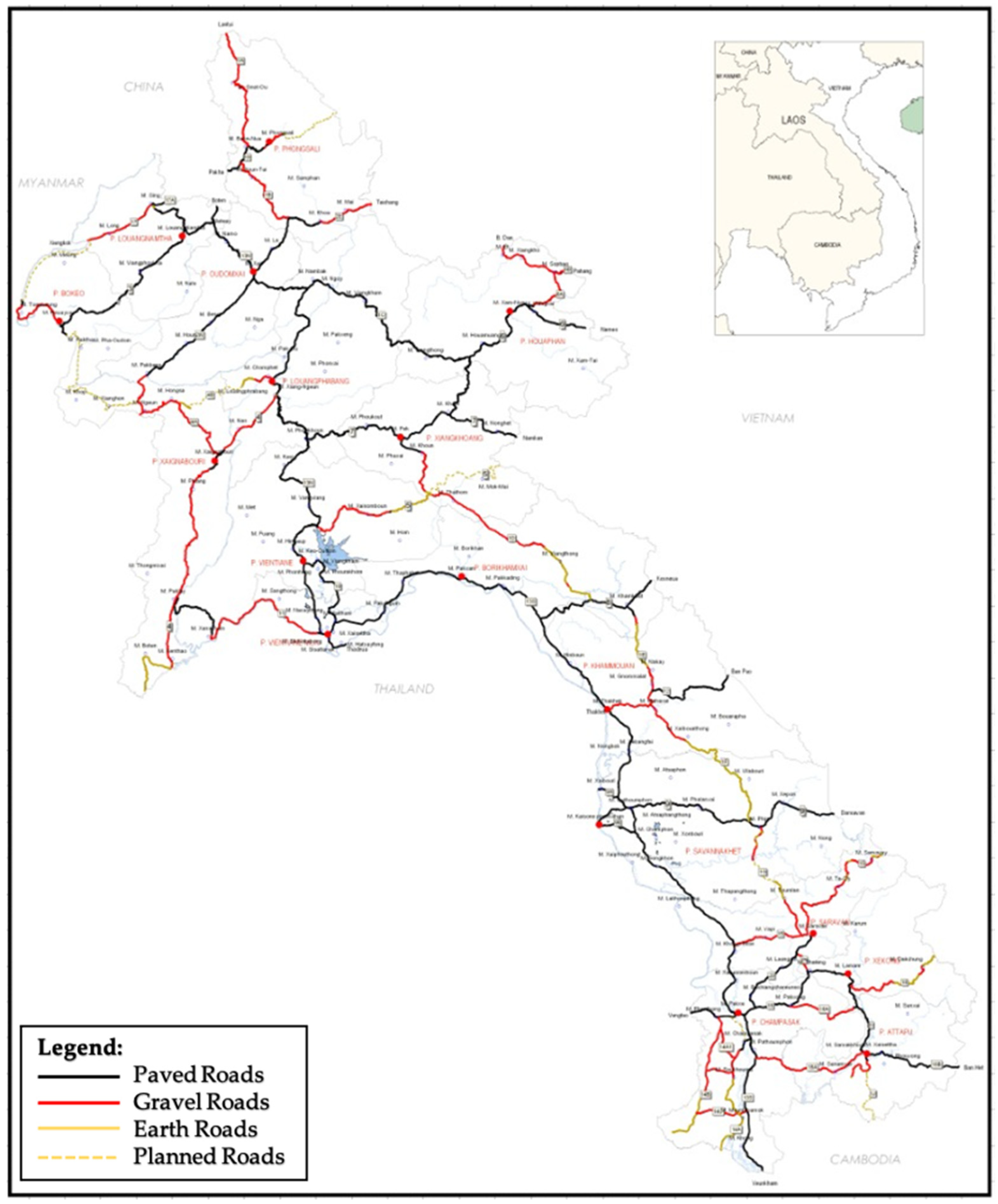
3.1. Area of Study
3.2. Model Variables’ Description
- IRIDBST is the predicted value of the IRI for DBST pavement sections (m/km);
- IRIAC is the predicted value of the IRI for AC pavement sections (m/km);
- Age is the pavement age since the last overlay to the day of the IRI reading (years);
- CESAL is the cumulative number of equivalent single axle loads that pavement experienced from the last overlay to the day of the IRI reading (104 axles/lane);
- YESAL is the average CESAL (CESAL/Age) that pavement experienced from the last overlay to the day of the IRI reading (104 axles/lane).
3.3. ANFIS Approach
3.3.1. Fuzzy Inference Systems
- Fuzzification requires converting crisp or classical data into fuzzy data or MFs;
- The fuzzy inference process connects MFs with fuzzy rules to derive the fuzzy output;
- Defuzzification which calculates each associated output.
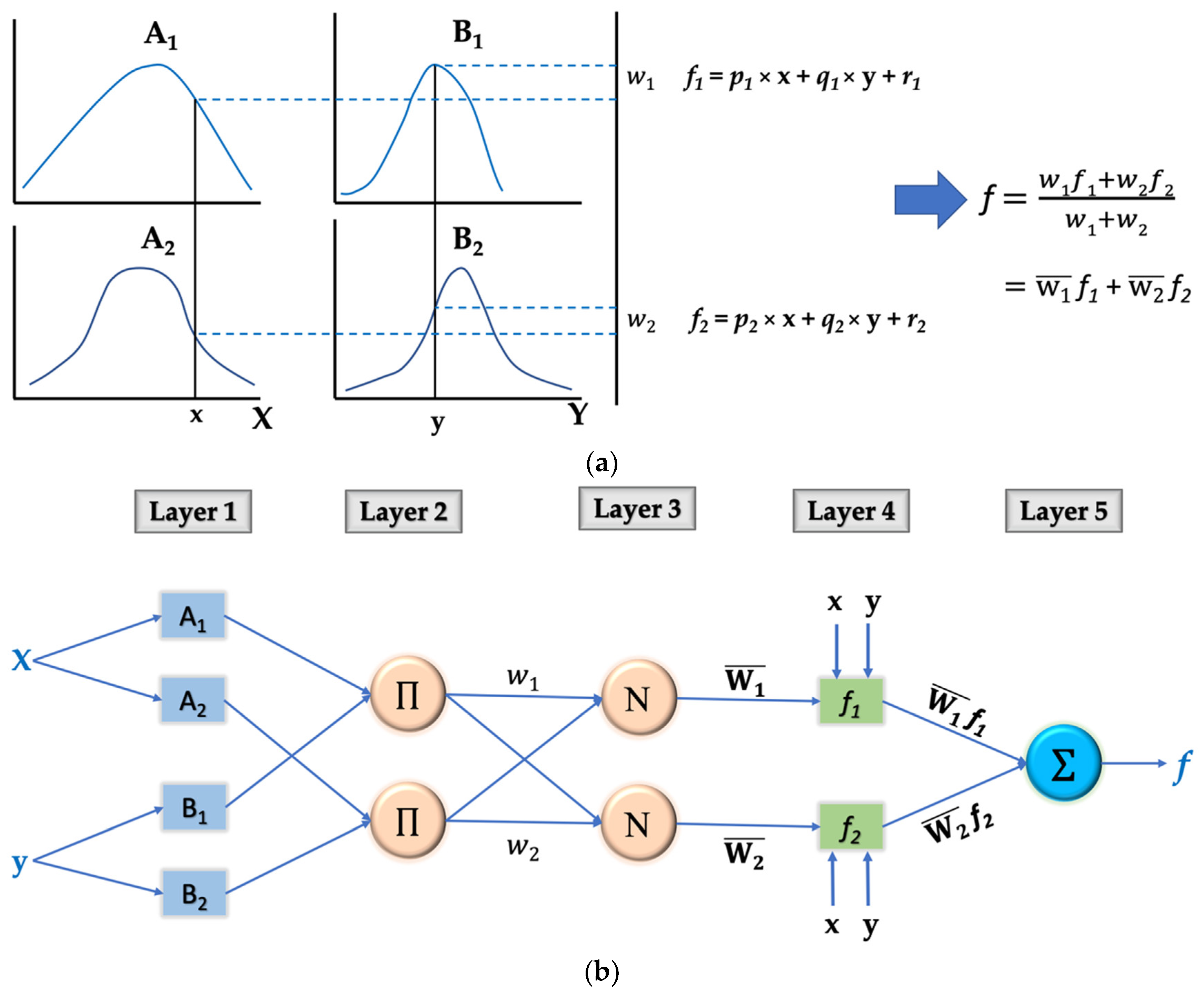
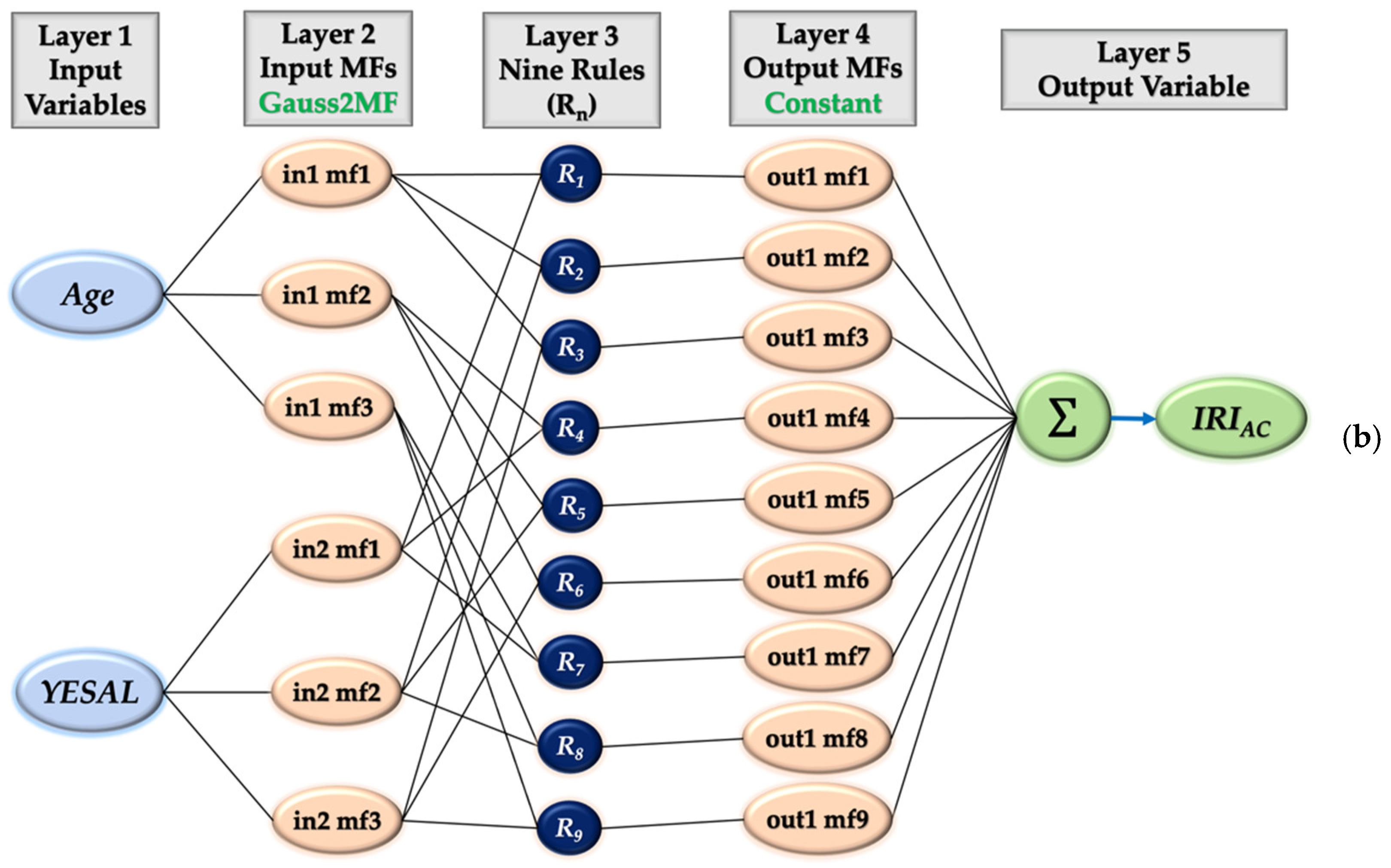
3.3.2. Architecture of ANFIS Model
- x and y are the inputs;
- Ai and Bi are fuzzy sets;
- fi is the output within the fuzzy region specified by the fuzzy rule;
- pi, qi, and ri are the design parameters that are determined during the training process.
3.3.3. Hybrid Learning Algorithm
3.4. Model Assessment Criteria
4. ANFIS Model Development
5. Result Analysis
6. Comparative Study
7. Study Limitations and Recommendations for Future Work
8. Conclusions
Author Contributions
Funding
Institutional Review Board Statement
Informed Consent Statement
Data Availability Statement
Acknowledgments
Conflicts of Interest
References
- AASTHO Pavement Management Guide, 2nd ed.; AASHTO: Washington, WA, USA, 2012.
- Pérez-Acebo, H.; Linares-Unamunzaga, A.; Rojí, E.; Gonzalo-Orden, H. IRI performance models for flexible pavements in two-lane roads until first maintenance and/or rehabilitation work. Coatings 2020, 10, 97. [Google Scholar] [CrossRef]
- Loprencipe, G.; Zoccali, P. Ride quality due to road surface irregularities: Comparison of different methods applied on a set of real road profiles. Coatings 2017, 7, 59. [Google Scholar] [CrossRef]
- ARA. Guide for Mechanistic-Empirical Design of New and Rehabiltated Pavement Structures; Appendix OO-1: Background and Preliminary Smoothness Prediction Models for Flexible Pavements; National Cooperative Highway Research Program: Champaign, IL, USA, 2001. [Google Scholar]
- Pérez-Acebo, H.; Bejan, S.; Gonzalo-Orden, H. Transition Probability Matrices for Flexible Pavement Deterioration Models with Half-Year Cycle Time. Int. J. Civ. Eng. 2018, 16, 1045–1056. [Google Scholar] [CrossRef]
- Kirbaş, U. IRI sensitivity to the influence of surface distress on flexible pavements. Coatings 2018, 8, 271. [Google Scholar] [CrossRef]
- Múčka, P. International Roughness Index specifications around the world. Road Mater. Pavement Des. 2017, 18, 929–965. [Google Scholar] [CrossRef]
- Zeiada, W.; Hamad, K.; Omar, M.; Underwood, B.S.; Khalil, M.A.; Karzad, A.S. Investigation and modelling of asphalt pavement performance in cold regions. Int. J. Pavement Eng. 2019, 20, 986–997. [Google Scholar] [CrossRef]
- Marcelino, P.; de Lurdes Antunes, M.; Fortunato, E.; Gomes, M.C. Machine learning approach for pavement performance prediction. Int. J. Pavement Eng. 2021, 22, 341–354. [Google Scholar] [CrossRef]
- Chai, G.; Akli, O.; Asmaniza, A.; Singh, M.; Chong, C.L. Calibration of HDM Model for the North South Expressway in Malaysia. In Proceedings of the 6th International Conference on Managing Pavements, Brisbane, QLD, Australia, 19–24 October 2004; pp. 1–10. [Google Scholar]
- Yogesh, U.S.; Jain, S.S.; Devesh, T. Adaptation of HDM-4 Tool for Strategic Analysis of Urban Roads Network. Transp. Res. Procedia 2016, 17, 71–80. [Google Scholar] [CrossRef]
- Bennett, C.R.; Paterson, W.D.O. A Guide to Calibration and Adaptation. In HDM 4—Highway Developmenet & Management Series; TRL: Paris, France, 2000; Volume 5. [Google Scholar]
- Braga, A.; Čygas, D. Adaptation of pavement deterioration models to lithuanian automobile roads. J. Civ. Eng. Manag. 2002, 8, 214–220. [Google Scholar] [CrossRef]
- Ognjenovic, S.; Krakutovski, Z.; Vatin, N. Calibration of the crack initiation model in HDM 4 on the highways and primary urban streets network in Macedonia. Procedia Eng. 2015, 117, 559–567. [Google Scholar] [CrossRef][Green Version]
- Jain, S.S.; Aggarwal, S.; Parida, M. HDM-4 pavement deterioration models for Indian national highway network. J. Transp. Eng. 2005, 131, 623–631. [Google Scholar] [CrossRef]
- Han, D.; Kobayashi, K.; Do, M. Improved calibration for HDM-4 implementation: A lesson from Korean experiences. Jsce 2009, 4. Available online: http://library.jsce.or.jp/jsce/open/00039/200911_no40/pdf/84.pdf (accessed on 22 January 2022).
- Han, D.; Kobayashi, K.; Do, M. Section-based multifunctional calibration method for pavement deterioration forecasting model. KSCE J. Civ. Eng. 2013, 17, 386–394. [Google Scholar] [CrossRef]
- La Torre, F.; Domenichini, L.; Darter, M.I. Roughness prediction model based on the artificial neural network approach. In Proceedings of the Fourth International Conference on Managing Pavements, Durban, South Africa, 17–21 May 1998; Volume 2. [Google Scholar]
- Lin, J.-D.; Yau, J.-T.; Hsiao, L.-H. Correlation analysis between international roughness index (IRI) and pavement distress by neural network. In Proceedings of the 82nd Annual Meeting of the Transportation Research Board, Washington, DC, USA, 12–16 January 2003; pp. 12–16. [Google Scholar]
- Hossain, M.; Gopisetti, L.S.P.; Miah, M.S. Artificial neural network modelling to predict international roughness index of rigid pavements. Int. J. Pavement Res. Technol. 2020, 13, 229–239. [Google Scholar] [CrossRef]
- Kaloop, M.; El-Badawy, S.; Ahn, J.; Sim, H.-B.; Hu, J.; Abd El-Hakim, R. A Hybrid Wavelet-Optimally-Pruned Extreme Learning Machine Model for the Estimation of International Roughness Index of Rigid Pavements. Int. J. Pavement Eng. 2020, 23, 1–15. [Google Scholar] [CrossRef]
- Nguyen, H.-L.; Pham, B.T.; Son, L.H.; Thang, N.T.; Ly, H.-B.; Le, T.-T.; Ho, L.S.; Le, T.-H.; Tien Bui, D. Adaptive network based fuzzy inference system with meta-heuristic optimizations for international roughness index prediction. Appl. Sci. 2019, 9, 4715. [Google Scholar] [CrossRef]
- Choi, J.H.; Adams, T.M.; Bahia, H.U. Pavement roughness modeling using back-propagation neural networks. Comput. Civ. Infrastruct. Eng. 2004, 19, 295–303. [Google Scholar] [CrossRef]
- Teomete, E.; Bayrak, M.B.; Agarwal, M. Use of Artificial Neural Networks for Predicting Rigid Pavement Roughness. In Proceedings of the 2004 Transportation Scholars ConferenceIowa State University, Ames, IA, USA, 19 November 2004. [Google Scholar]
- Chou, S.F.; Pellinen, T.K. Assessment of construction smoothness specification pay factor limits using artificial neural network modeling. J. Transp. Eng. 2005, 131, 563–570. [Google Scholar] [CrossRef]
- Abd El-Hakim, R.; El-Badawy, S. International roughness index prediction for rigid pavements: An artificial neural network application. Adv. Mater. Res. 2013, 723, 854–860. [Google Scholar] [CrossRef]
- Ziari, H.; Sobhani, J.; Ayoubinejad, J.; Hartmann, T. Prediction of IRI in short and long terms for flexible pavements: ANN and GMDH methods. Int. J. Pavement Eng. 2015, 17, 776–788. [Google Scholar] [CrossRef]
- Mazari, M.; Rodriguez, D.D. Prediction of pavement roughness using a hybrid gene expression programming-neural network technique. J. Traffic Transp. Eng. 2016, 3, 448–455. [Google Scholar] [CrossRef]
- Abdelaziz, N.; Abd El-Hakim, R.T.; El-Badawy, S.M.; Afify, H.A. International roughness index prediction model for flexible pavements. Int. J. Pavement Eng. 2020, 21, 88–99. [Google Scholar] [CrossRef]
- Georgiou, P.; Plati, C.; Loizos, A. Soft Computing Models to Predict Pavement Roughness: A Comparative Study. Adv. Civ. Eng. 2018, 2018, 5939806. [Google Scholar] [CrossRef]
- Terzi, S. Modeling for pavement roughness using the ANFIS approach. Adv. Eng. Softw. 2013, 57, 59–64. [Google Scholar] [CrossRef]
- Gharieb, M.; Nishikawa, T. Development of Roughness Prediction Models for Laos National Road Network. CivilEng 2021, 2, 158–173. [Google Scholar] [CrossRef]
- Laos Ministry of Public Works and Transport, Department of Roads. Summary of Road Network Statistics Year; Laos Ministry of Public Works and Transport: Vientiane, Laos, 2020.
- Tarno; Rusgiyono, A.; Sugito. Adaptive Neuro Fuzzy Inference System (ANFIS) approach for modeling paddy production data in Central Java. J. Phys. Conf. Ser. 2019, 1217, 012083. [Google Scholar] [CrossRef]
- Naresh, C.; Bose, P.S.C.; Rao, C.S.P. Artificial neural networks and adaptive neuro-fuzzy models for predicting WEDM machining responses of Nitinol alloy: Comparative study. SN Appl. Sci. 2020, 2, 1–23. [Google Scholar] [CrossRef]
- Jang, J.-S. ANFIS: Adaptive-network-based fuzzy inference system. IEEE Trans. Syst. Man. Cybern. 1993, 23, 665–685. [Google Scholar] [CrossRef]
- Jang, J.-S.R.; Sun, C.-T.; Mizutani, E. Neuro-fuzzy and soft computing-a computational approach to learning and machine intelligence [Book Review]. IEEE Trans. Automat. Contr. 1997, 42, 1482–1484. [Google Scholar] [CrossRef]
- Zadeh, L.A. Fuzzy sets. In Fuzzy Sets, Fuzzy Logic, and Fuzzy Systems: Selected Papers by Lotfi A Zadeh; World Scientific: River Edge, NJ, USA, 1996; pp. 394–432. [Google Scholar]
- Çekmiş, A.; Hacıhasanoğlu, I.; Ostwald, M.J. A computational model for accommodating spatial uncertainty: Predicting inhabitation patterns in open-planned spaces. Build. Environ. 2014, 73, 115–126. [Google Scholar] [CrossRef]
- Sivanandam, S.N.; Sumathi, S.; Deepa, S.N. Fuzzy rule-based system. In Introduction to Fuzzy Logic Using Matlab; Springer: Berlin, Germany, 2007; pp. 113–149. [Google Scholar]
- Cabalar, A.F.; Cevik, A.; Gokceoglu, C. Some applications of adaptive neuro-fuzzy inference system (ANFIS) in geotechnical engineering. Comput. Geotech. 2012, 40, 14–33. [Google Scholar] [CrossRef]
- Singh, R.; Kainthola, A.; Singh, T.N. Estimation of elastic constant of rocks using an ANFIS approach. Appl. Soft Comput. 2012, 12, 40–45. [Google Scholar] [CrossRef]
- Takagi, T.; Sugeno, M. Fuzzy identification of systems and its applications to modeling and control. IEEE Trans. Syst. Man. Cybern. 1985, SMC-15, 116–132. [Google Scholar] [CrossRef]
- Finol, J.; Guo, Y.K.; Jing, X.D. A rule based fuzzy model for the prediction of petrophysical rock parameters. J. Pet. Sci. Eng. 2001, 29, 97–113. [Google Scholar] [CrossRef]
- Manual, M. Fuzzy Logic ToolboxTM User’s Guide; MathWorks: Natick, MA, USA, 2009. [Google Scholar]
- Yaseen, Z.M.; Ebtehaj, I.; Bonakdari, H.; Deo, R.C.; Mehr, A.D.; Mohtar, W.H.M.W.; Diop, L.; El-Shafie, A.; Singh, V.P. Novel approach for streamflow forecasting using a hybrid ANFIS-FFA model. J. Hydrol. 2017, 554, 263–276. [Google Scholar] [CrossRef]
- Shah, M.I.; Abunama, T.; Javed, M.F.; Bux, F.; Aldrees, A.; Tariq, M.A.U.R.; Mosavi, A. Modeling Surface Water Quality Using the Adaptive Neuro-Fuzzy Inference System Aided by Input Optimization. Sustainability 2021, 13, 4576. [Google Scholar] [CrossRef]
- Vasileva-Stojanovska, T.; Vasileva, M.; Malinovski, T.; Trajkovik, V. An ANFIS model of quality of experience prediction in education. Appl. Soft Comput. 2015, 34, 129–138. [Google Scholar] [CrossRef]
- Tiwari, S.; Babbar, R.; Kaur, G. Performance evaluation of two ANFIS models for predicting water quality Index of River Satluj (India). Adv. Civ. Eng. 2018, 2018, 8971079. [Google Scholar] [CrossRef]
- Hamdi; Hadiwardoyo, S.P.; Correia, A.G.; Pereira, P.; Cortez, P. Prediction of surface distress using neural networks. AIP Conf. Proc. 2017, 1855, 040006. [Google Scholar] [CrossRef]
- Al-Hmouz, A.; Shen, J.; Al-Hmouz, R.; Yan, J. Modeling and simulation of an adaptive neuro-fuzzy inference system (ANFIS) for mobile learning. IEEE Trans. Learn. Technol. 2011, 5, 226–237. [Google Scholar] [CrossRef]
- Odoki, J.B.; Kerali, G.R.H. Volume Four: Analytical Framework and Model Descriptions. In Highway Development and Management Model HDM-4 (Version 1.2); TRL: Paris, France, 2001. [Google Scholar]
- Sandra, A.K.; Sarkar, A.K. Development of a model for estimating International Roughness Index from pavement distresses. Int. J. Pavement Eng. 2013, 14, 715–724. [Google Scholar] [CrossRef]
- Makendran, C.; Murugasan, R.; Velmurugan, S. Performance prediction modelling for flexible pavement on low volume roads using multiple linear regression analysis. J. Appl. Math. 2015, 2015, 192485. [Google Scholar] [CrossRef]


| Authors, Year | Pavement Type | Source of Data * | Modeling * | Independent Variables * | Model Performance |
|---|---|---|---|---|---|
| Terzi, 2013 [31] | Flexible Pavement | LTPP-IMS Database | ANFIS | AGE, SN, CESAL | R2 = 0.97 |
| Nguyen, 2019 [22] | AC pavement | 2811 Samples as a case study in the North of Vietnam | PSOANFIS | Road Length, Analysis Area, Summed Cracks, Maximum Depth of Rut, Average Depth of Rut | R = 0.888, RMSE = 0.145 |
| GANFIS | R = 0.872, RMSE = 0.155 | ||||
| FAANFIS | R = 0.849, RMSE = 0.170 | ||||
| ANN | R = 0.804, RMSE = 0.186 | ||||
| Chou, 2005 [25] | PCC | Indian PMS database | ANN | IRI0, AGE, FI, AP, F/T, ESAL | R2 = 0.98, RMSE = 0.074, N = 90 |
| Asphalt overlay on concrete pavement | R2 = 0.88, RMSE = 0.124, N = 1080 | ||||
| HMA | R2 = 0.90, RMSE = 0.121, N = 640 | ||||
| Ziari, 2015 [27] | AC over granular base | LTPP database | ANN | AGE, AAP, AAT, AAFI, AADT, AADTT, ESAL, STH, PTH | R2 = 0.90, RMSE = 0.09, MAPE = 5.54, N = 205 |
| GMDH | R2 = 0.63, RMSE = 0.405, MAPE = 28.62, N = 205 | ||||
| Mazari, 2016 [28] | AC over unbound granular layers | LTPP database | Hybrid GEP-ANN | SN, AGE, CESAL | R = 0.99, RMSE = 0.049, N = 95 |
| Georgiou, 2018 [30] | AC pavement | Direct field measurement, Greece | ANN | CR, RUT, PH | R2 = 0.96, MAE = 6.9%, RMSPE = 8.3% |
| SVM | R2 = 0.93, MAE = 7.7%, RMSPE = 8.9% | ||||
| Kaloop, 2020 [21] | JPCP | LTPP GPS-3 database | ANN | IRI0, FI, TFAULT | r = 0.80, MAE = 0.37, RMSE = 0.49, N = 184 |
| WOPELM | r = 0.92, MAE = 0.23, RMSE = 0.24, N = 184 |
| Variable | Training (70%) | Checking (15%) | Test (15%) | All Data | ||||||||||||
|---|---|---|---|---|---|---|---|---|---|---|---|---|---|---|---|---|
| Min | Max | Mean | Std | Min | Max | Mean | Std | Min | Max | Mean | Std | Min | Max | Mean | Std | |
| DBST Model | ||||||||||||||||
| Age | 0.10 | 13.39 | 5.50 | 3.76 | 0.11 | 12.53 | 7.25 | 3.60 | 1.58 | 14.10 | 7.27 | 3.22 | 0.10 | 14.10 | 6.03 | 3.73 |
| CESAL | 0.02 | 99.26 | 12.44 | 15.71 | 0.07 | 56.25 | 12.79 | 13.52 | 0.25 | 87.07 | 17.75 | 22.03 | 0.02 | 99.26 | 13.28 | 16.55 |
| IRI | 2.28 | 8.83 | 4.92 | 1.42 | 2.20 | 8.12 | 5.43 | 1.46 | 3.49 | 8.91 | 5.53 | 1.39 | 2.20 | 8.91 | 5.09 | 1.44 |
| AC Model | ||||||||||||||||
| Age | 0.09 | 13.08 | 5.81 | 3.37 | 0.09 | 11.76 | 6.09 | 3.69 | 0.18 | 11.53 | 6.44 | 3.66 | 0.09 | 13.08 | 5.95 | 3.44 |
| YESAL | 0.03 | 13.15 | 4.24 | 3.00 | 0.15 | 15.13 | 4.87 | 3.65 | 0.61 | 20.53 | 4.85 | 4.55 | 0.03 | 20.53 | 4.42 | 3.34 |
| IRI | 1.47 | 5.46 | 3.47 | 0.99 | 1.90 | 5.17 | 3.71 | 1.06 | 1.87 | 5.31 | 3.67 | 1.12 | 1.47 | 5.46 | 3.54 | 1.02 |
| DBST Model | AC Model | ||||||||||
|---|---|---|---|---|---|---|---|---|---|---|---|
| MF No. | MF Type | Root Mean Squared Error (RMSE) | MF No. | MF Type | Root Mean Squared Error (RMSE) | ||||||
| Training | Checking | Testing | Overall | Training | Checking | Testing | Overall | ||||
| 2–2 | Trimf | 0.440 | 0.541 | 0.448 | 0.456 | 2–2 | Trimf | 0.382 | 0.237 | 0.405 | 0.364 |
| Trapmf | 0.518 | 0.671 | 0.557 | 0.546 | Trapmf | 0.404 | 0.228 | 0.468 | 0.387 | ||
| Gbellmf | 0.480 | 0.607 | 0.478 | 0.498 | Gbellmf | 0.399 | 0.230 | 0.466 | 0.384 | ||
| Gaussmf | 0.442 | 0.539 | 0.432 | 0.455 | Gaussmf | 0.396 | 0.227 | 0.433 | 0.377 | ||
| Gauss2mf | 0.436 | 0.577 | 0.445 | 0.458 | Gauss2mf | 0.388 | 0.235 | 0.467 | 0.377 | ||
| Pimf | 0.664 | 0.804 | 0.673 | 0.686 | Pimf | 0.447 | 0.279 | 0.498 | 0.430 | ||
| Dsigmf | 0.627 | 0.757 | 0.575 | 0.638 | Dsigmf | 0.418 | 0.246 | 0.480 | 0.402 | ||
| Psigmf | 0.627 | 0.757 | 5.696 | 1.400 | Psigmf | 0.425 | 0.246 | 0.485 | 0.407 | ||
| 3–3 | Trimf | 0.405 | 0.502 | 0.408 | 0.420 | 3–3 * | Trimf | 0.375 | 0.224 | 0.578 | 0.383 |
| Trapmf | 0.400 | 0.498 | 1.365 | 0.558 | Trapmf | 0.439 | 0.442 | 0.678 | 0.474 | ||
| Gbellmf | 0.458 | 0.590 | 0.524 | 0.487 | Gbellmf | 0.399 | 0.320 | 0.471 | 0.397 | ||
| Gaussmf | 0.367 | 0.477 | 0.355 | 0.382 | Gaussmf | 0.382 | 0.265 | 0.432 | 0.372 | ||
| Gauss2mf | 0.408 | 0.551 | 0.410 | 0.430 | Gauss2mf ** | 0.355 | 0.264 | 0.439 | 0.354 | ||
| Pimf | 0.463 | 0.601 | 0.483 | 0.486 | Pimf | 0.472 | 0.472 | 0.705 | 0.507 | ||
| Dsigmf | 0.428 | 0.556 | 0.641 | 0.479 | Dsigmf | 0.446 | 0.430 | 0.550 | 0.459 | ||
| Psigmf | 0.429 | 0.558 | 0.709 | 0.490 | Psigmf | 0.446 | 0.430 | 0.550 | 0.459 | ||
| 2–3 | Trimf | 0.438 | 0.530 | 0.434 | 0.451 | 2–3 | Trimf | 0.378 | 0.232 | 0.584 | 0.387 |
| Trapmf | 0.497 | 0.606 | 0.517 | 0.516 | Trapmf | 0.447 | 0.243 | 0.570 | 0.435 | ||
| Gbellmf | 0.495 | 0.607 | 0.521 | 0.516 | Gbellmf | 0.410 | 0.230 | 0.422 | 0.385 | ||
| Gaussmf | 0.501 | 0.599 | 0.502 | 0.516 | Gaussmf | 0.396 | 0.225 | 0.419 | 0.374 | ||
| Gauss2mf | 0.631 | 0.736 | 0.646 | 0.649 | Gauss2mf | 0.400 | 0.238 | 0.414 | 0.378 | ||
| Pimf | 0.620 | 0.756 | 0.658 | 0.646 | Pimf | 0.441 | 0.247 | 0.572 | 0.432 | ||
| Dsigmf | 0.594 | 0.711 | 0.539 | 0.603 | Dsigmf | 0.428 | 0.244 | 0.418 | 0.399 | ||
| Psigmf | 0.589 | 0.709 | 0.542 | 0.600 | Psigmf | 0.426 | 0.244 | 0.418 | 0.398 | ||
| 3–2 * | Trimf | 0.380 | 0.488 | 0.391 | 0.397 | 3–2 | Trimf | 0.384 | 0.226 | 0.383 | 0.361 |
| Trapmf | 0.469 | 0.575 | 0.523 | 0.492 | Trapmf | 0.370 | 0.271 | 0.474 | 0.371 | ||
| Gbellmf ** | 0.357 | 0.449 | 0.363 | 0.372 | Gbellmf | 0.405 | 0.245 | 0.459 | 0.389 | ||
| Gaussmf | 0.382 | 0.493 | 0.359 | 0.395 | Gaussmf | 0.398 | 0.232 | 0.417 | 0.376 | ||
| Gauss2mf | 0.412 | 0.488 | 0.422 | 0.425 | Gauss2mf | 0.389 | 0.245 | 0.456 | 0.378 | ||
| Pimf | 0.526 | 0.685 | 0.558 | 0.554 | Pimf | 0.441 | 0.308 | 0.545 | 0.437 | ||
| Dsigmf | 0.458 | 0.611 | 0.490 | 0.485 | Dsigmf | 0.371 | 0.257 | 0.444 | 0.365 | ||
| Psigmf | 0.465 | 0.625 | 0.499 | 0.494 | Psigmf | 0.367 | 0.258 | 0.440 | 0.362 | ||
| 4–4 | Trimf | 0.384 | 0.446 | 0.385 | 0.394 | 4–4 | Trimf | 0.362 | 0.263 | 0.582 | 0.379 |
| Trapmf | 0.463 | 0.500 | 0.912 | 0.535 | Trapmf | 0.363 | 0.248 | 0.627 | 0.385 | ||
| Gbellmf | 0.415 | 0.466 | 0.532 | 0.440 | Gbellmf | 0.350 | 0.310 | 0.457 | 0.360 | ||
| Gaussmf | 0.397 | 0.543 | 0.451 | 0.427 | Gaussmf | 0.348 | 0.386 | 0.439 | 0.367 | ||
| Gauss2mf | 0.459 | 0.513 | 7.188 | 1.468 | Gauss2mf | 0.357 | 0.246 | 0.658 | 0.385 | ||
| Pimf | 0.495 | 0.555 | 1.219 | 0.611 | Pimf | 0.362 | 0.254 | 0.629 | 0.385 | ||
| Dsigmf | 0.456 | 0.509 | 4.497 | 1.065 | Dsigmf | 0.357 | 0.245 | 0.763 | 0.400 | ||
| Psigmf | 0.456 | 0.509 | 4.497 | 1.065 | Psigmf | 0.357 | 0.245 | 0.863 | 0.415 | ||
| 5–5 | Trimf | 0.359 | 0.419 | 0.632 | 0.408 | 5–5 | Trimf | 0.328 | 0.278 | 0.887 | 0.403 |
| Trapmf | 0.384 | 0.464 | 0.754 | 0.451 | Trapmf | 0.321 | 0.344 | 0.908 | 0.411 | ||
| Gbellmf | 0.366 | 0.425 | 12.739 | 2.215 | Gbellmf | 0.302 | 0.300 | 0.924 | 0.393 | ||
| Gaussmf | 0.360 | 0.421 | 4.438 | 0.976 | Gaussmf | 0.305 | 0.278 | 1.000 | 0.403 | ||
| Gauss2mf | 0.385 | 0.449 | 0.738 | 0.447 | Gauss2mf | 0.320 | 0.412 | 1.433 | 0.498 | ||
| Pimf | 0.400 | 0.466 | 0.789 | 0.467 | Pimf | 0.335 | 0.548 | 0.630 | 0.410 | ||
| Dsigmf | 0.382 | 0.445 | 0.514 | 0.411 | Dsigmf | 0.318 | 0.379 | 1.043 | 0.433 | ||
| Psigmf | 0.382 | 0.445 | 0.514 | 0.411 | Psigmf | 0.318 | 0.379 | 1.043 | 0.433 | ||
| Description | DBST | AC |
|---|---|---|
| No. of Inputs | 2 | 2 |
| No. of Outputs | 1 | 1 |
| No. of Training dataset | 189 | 86 |
| No. of Checking dataset | 40 | 18 |
| No. of Testing dataset | 40 | 18 |
| Input MF No. | 3 (AGE) 2 (CESAL) | 3 (AGE) 3 (YESAL) |
| MF Type—Inputs | Gbellmf | Gauss2mf |
| MF Type—Outputs | Constant | Constant |
| Rules No. | 6 | 9 |
| Optimum Epoch No. | 335 | 250 |
| Learning Algorism | Hybrid | Hybrid |
| RMSE—Training Data | 0.357 | 0.355 |
| RMSE—Checking Data | 0.449 | 0.206 |
| RMSE—Testing Data | 0.363 | 0.320 |
| RMSE—Overall Data | 0.373 | 0.357 |
| Parameter | DBST Model | AC Model | ||||||
|---|---|---|---|---|---|---|---|---|
| Training | Checking | Testing | All | Training | Checking | Testing | All | |
| n | 189 | 40 | 40 | 269 | 86 | 18 | 18 | 122 |
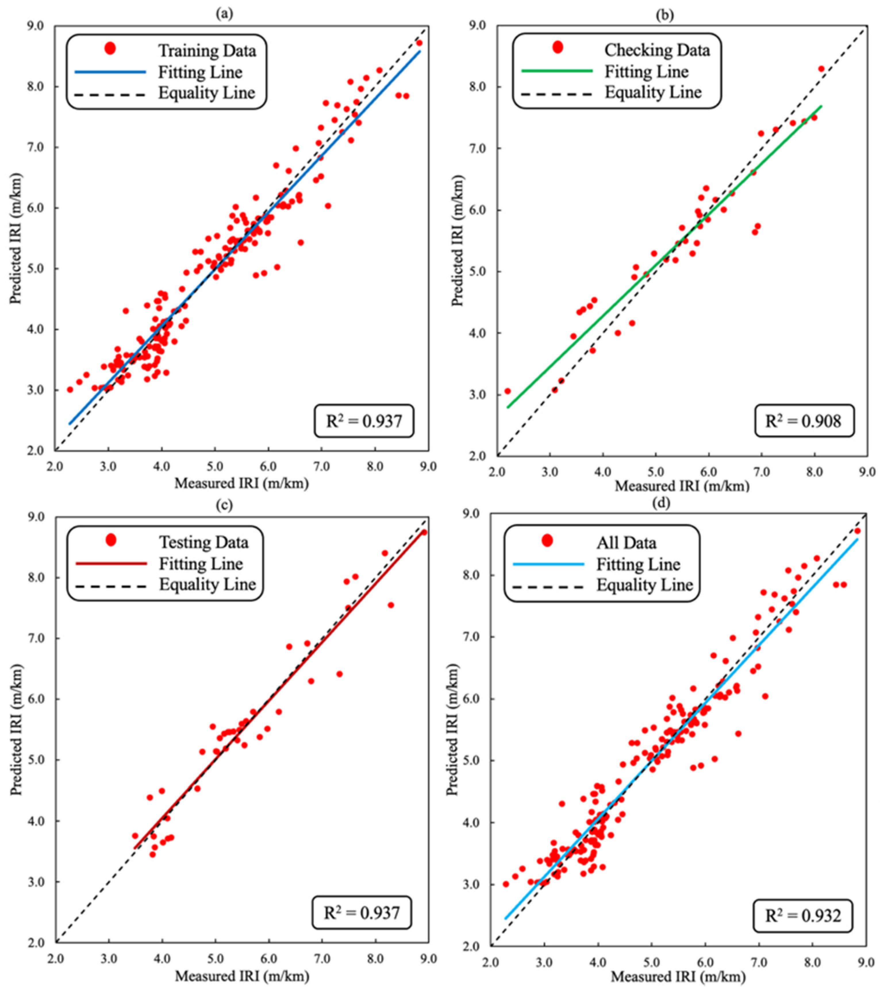
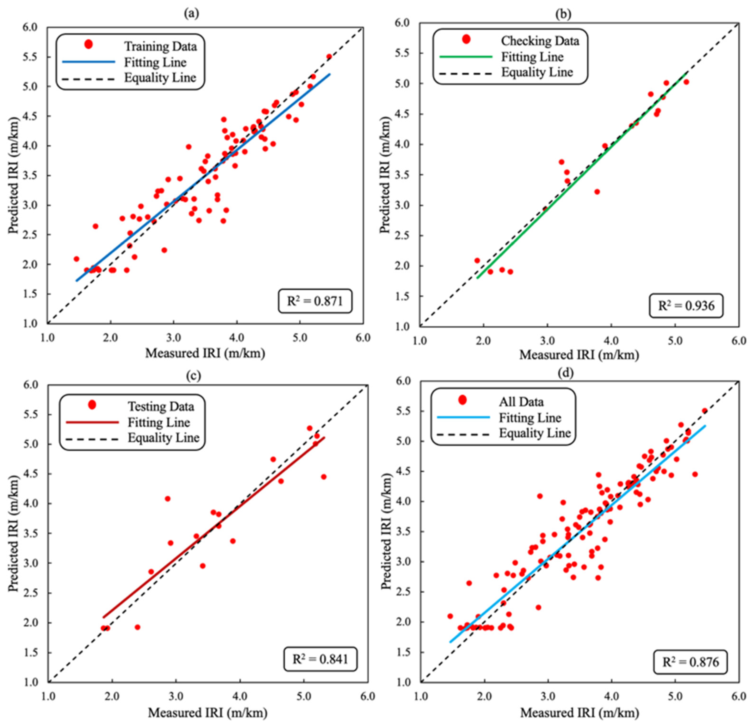
| R2 | 0.937 | 0.908 | 0.937 | 0.932 | 0.871 | 0.936 | 0.841 | 0.876 |
| MAE | 0.269 | 0.335 | 0.298 | 0.283 | 0.267 | 0.264 | 0.439 | 0.266 |
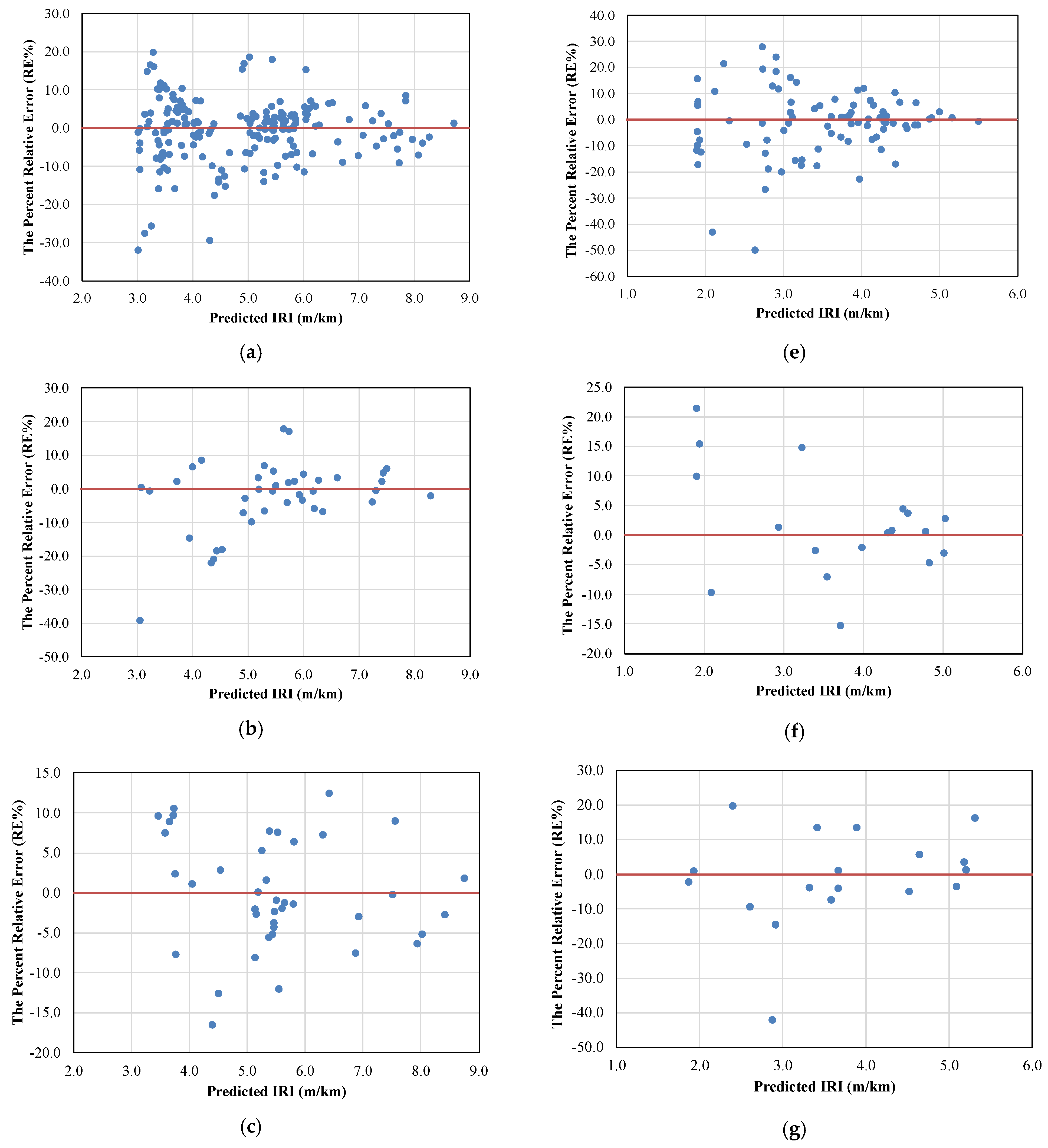
| RMSPE | 8.163 | 10.722 | 6.861 | 8.421 | 12.730 | 9.039 | 13.485 | 12.374 |
| Parameter | DBST Model | AC Model | ||
|---|---|---|---|---|
| ANFIS | MLR | ANFIS | MLR | |
| n | 189 | 215 | 86 | 98 |
| R2 | 0.937 | 0.892 | 0.871 | 0.847 |
| MAE | 0.269 | 0.336 | 0.267 | 0.314 |
| RMSPE | 8.163 | 9.626 | 12.730 | 12.186 |
Publisher’s Note: MDPI stays neutral with regard to jurisdictional claims in published maps and institutional affiliations. |
© 2022 by the authors. Licensee MDPI, Basel, Switzerland. This article is an open access article distributed under the terms and conditions of the Creative Commons Attribution (CC BY) license (https://creativecommons.org/licenses/by/4.0/).
Share and Cite
Gharieb, M.; Nishikawa, T.; Nakamura, S.; Thepvongsa, K. Application of Adaptive Neuro–Fuzzy Inference System for Forecasting Pavement Roughness in Laos. Coatings 2022, 12, 380. https://doi.org/10.3390/coatings12030380
Gharieb M, Nishikawa T, Nakamura S, Thepvongsa K. Application of Adaptive Neuro–Fuzzy Inference System for Forecasting Pavement Roughness in Laos. Coatings. 2022; 12(3):380. https://doi.org/10.3390/coatings12030380
Chicago/Turabian StyleGharieb, Mohamed, Takafumi Nishikawa, Shozo Nakamura, and Khampaseuth Thepvongsa. 2022. "Application of Adaptive Neuro–Fuzzy Inference System for Forecasting Pavement Roughness in Laos" Coatings 12, no. 3: 380. https://doi.org/10.3390/coatings12030380
APA StyleGharieb, M., Nishikawa, T., Nakamura, S., & Thepvongsa, K. (2022). Application of Adaptive Neuro–Fuzzy Inference System for Forecasting Pavement Roughness in Laos. Coatings, 12(3), 380. https://doi.org/10.3390/coatings12030380