
Time Evolution of Bacterial Resistance Observed with Principal Component Analysis

 ,
,  , , , and
Abstract
1. Introduction
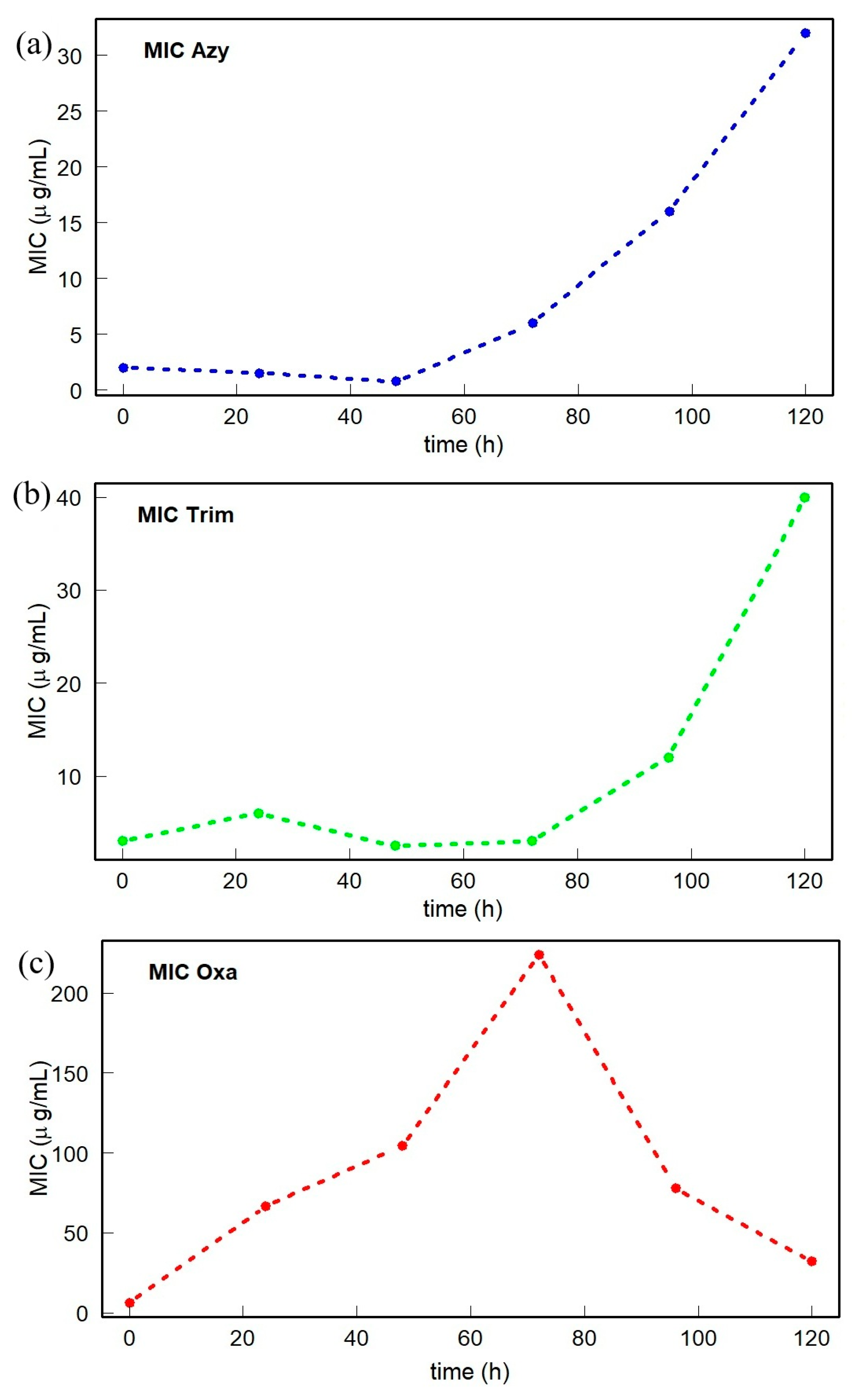
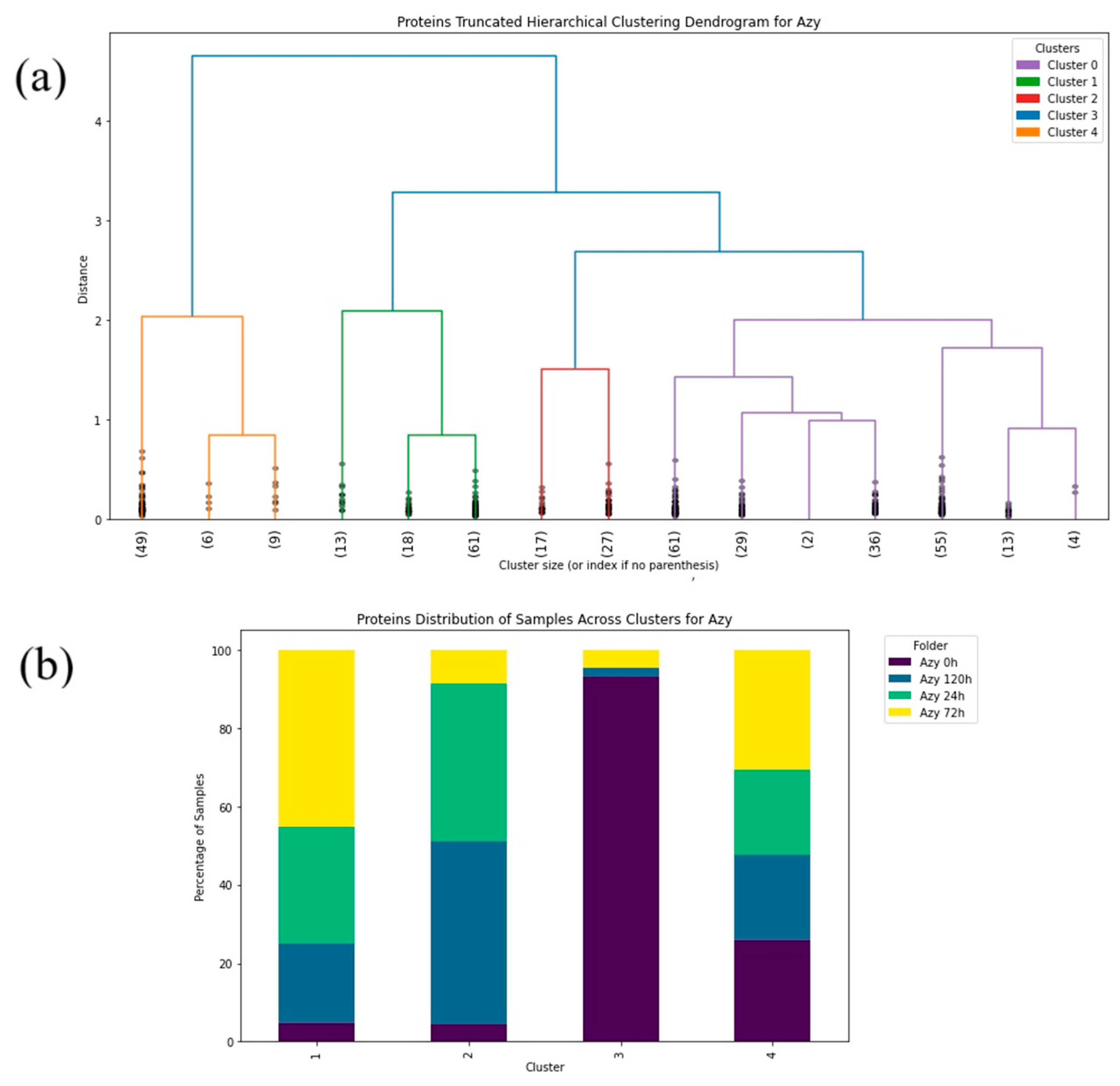
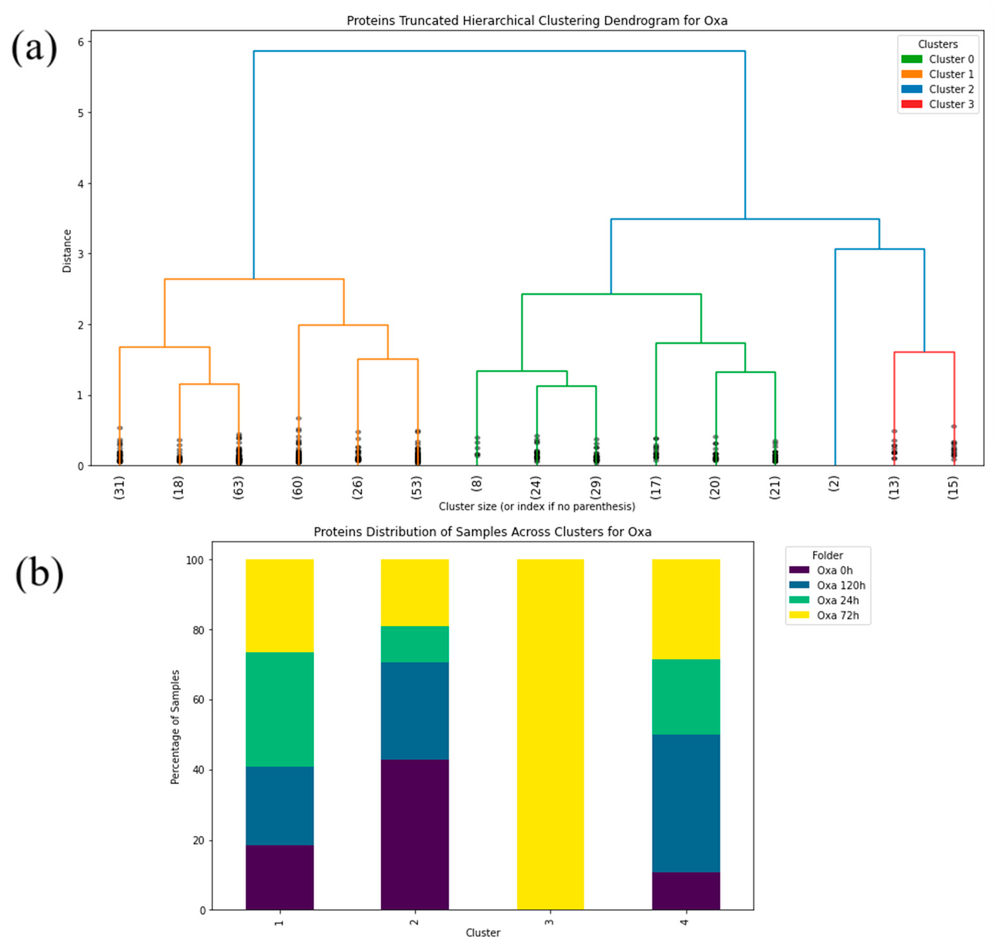
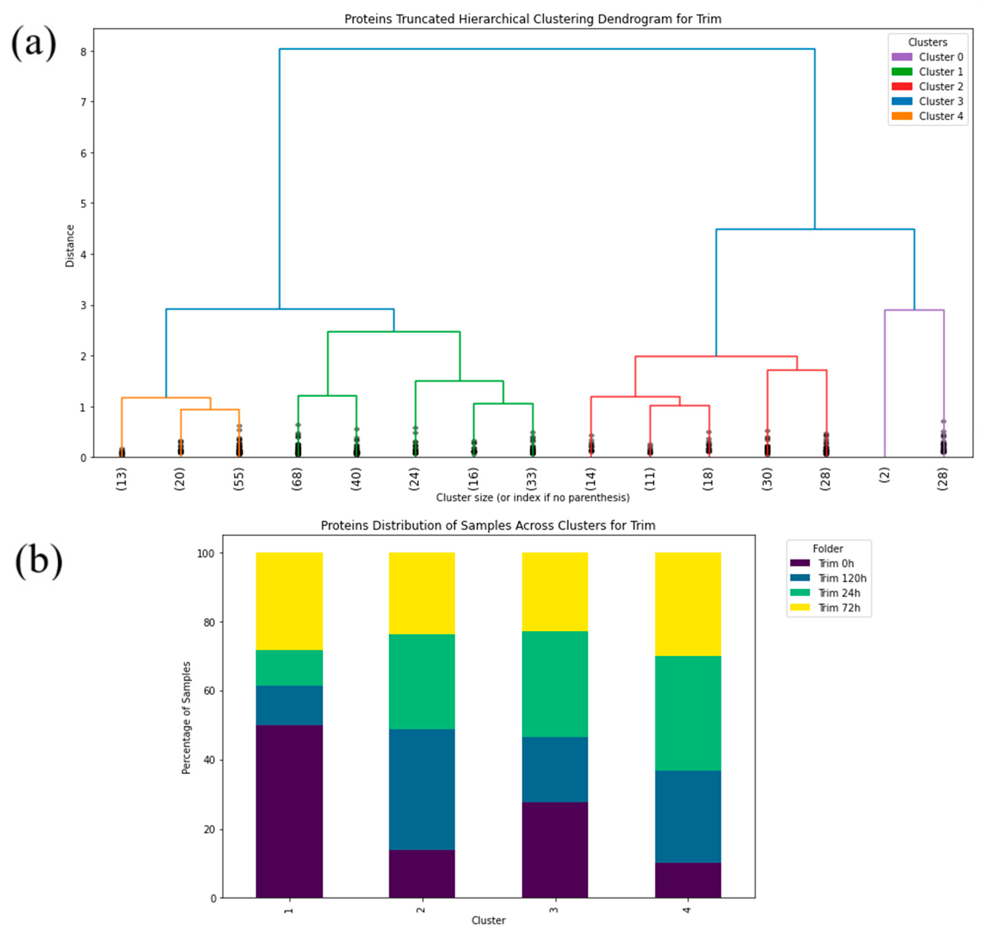
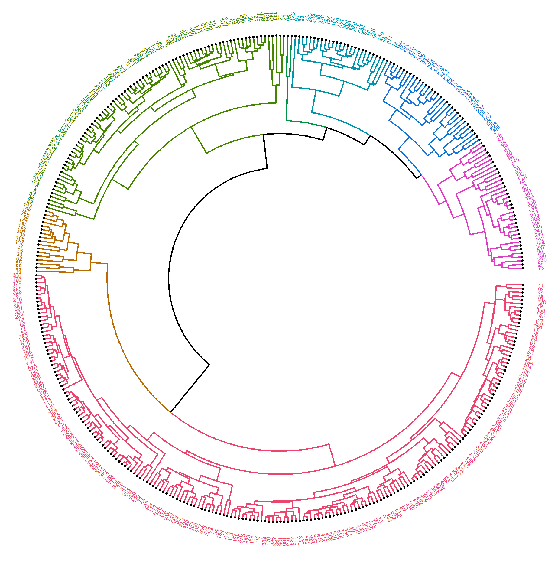
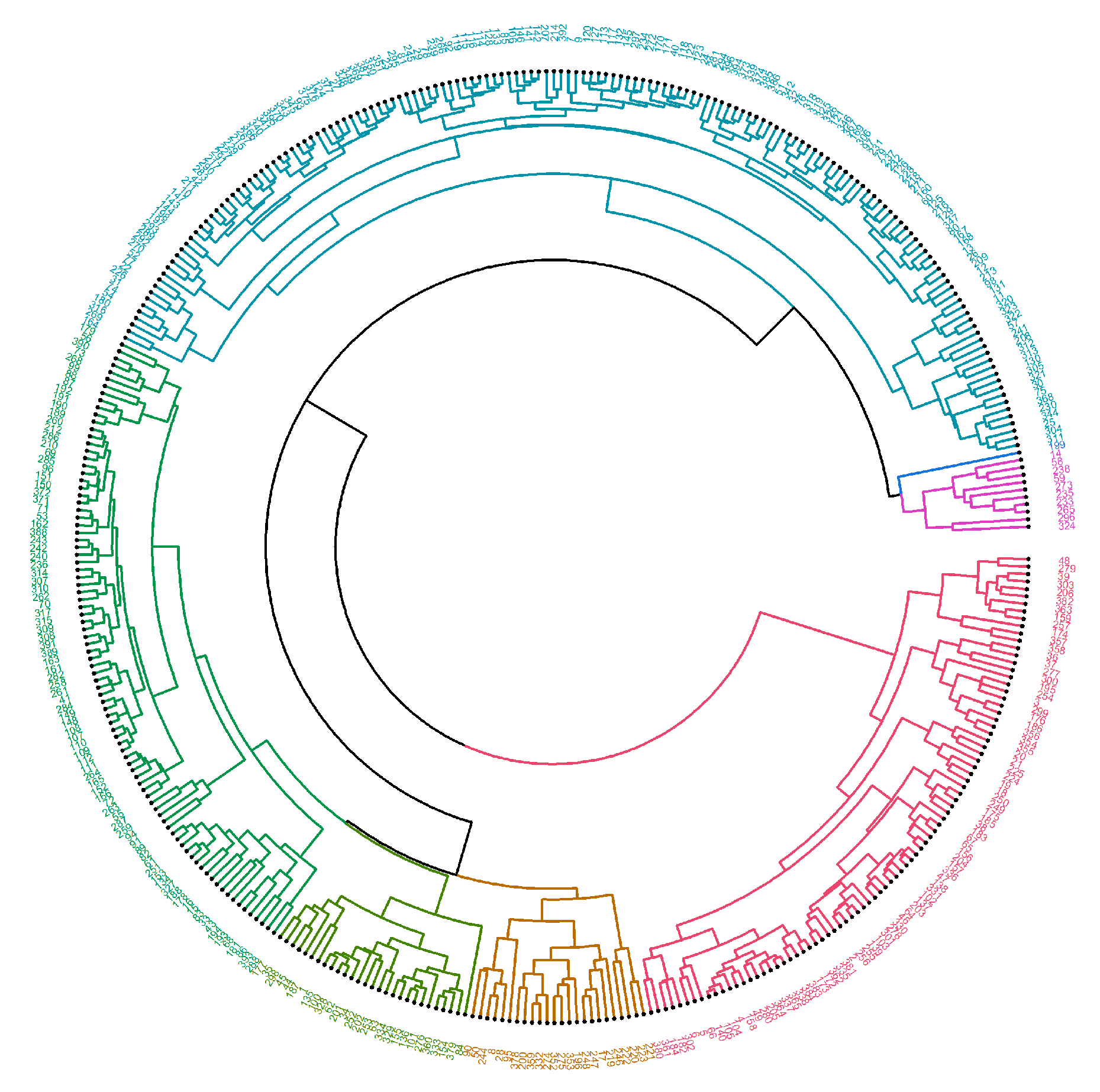
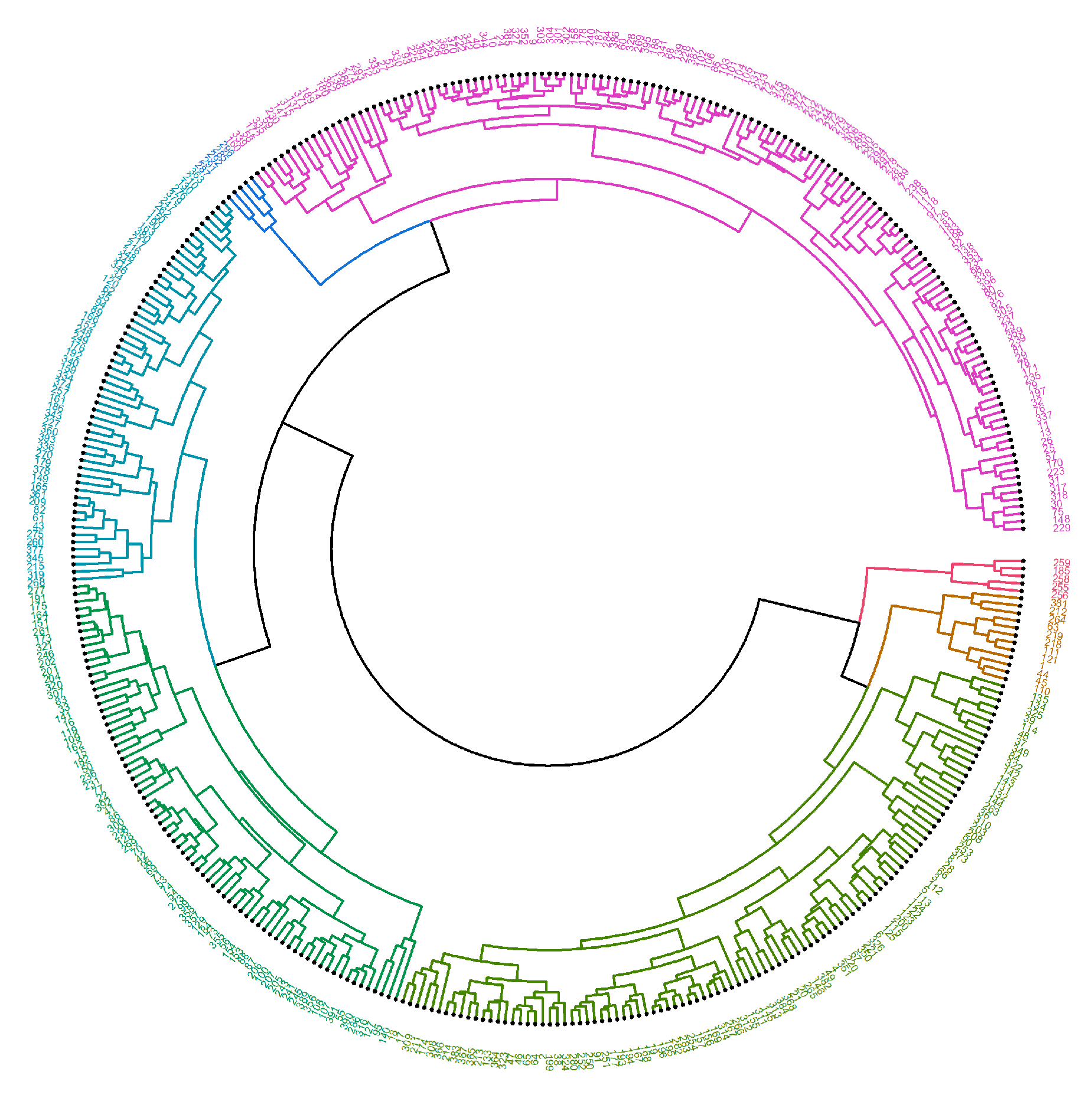
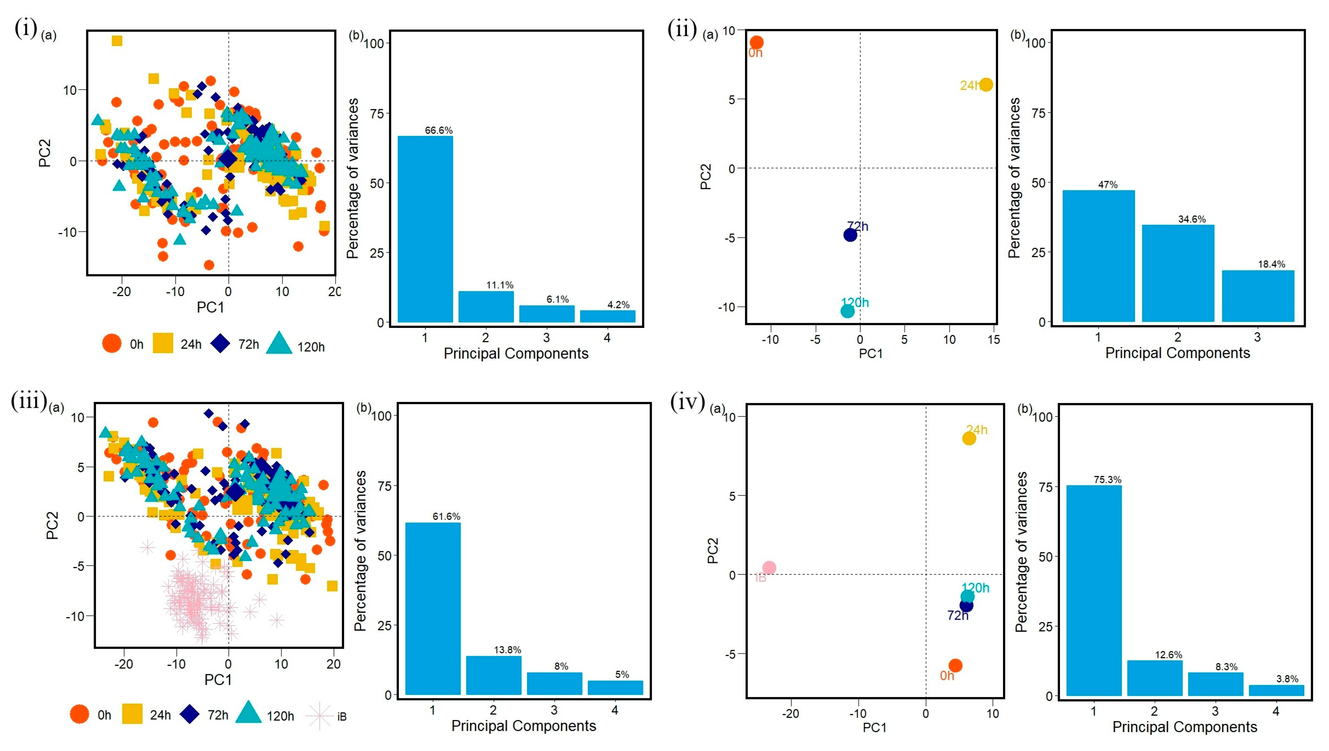
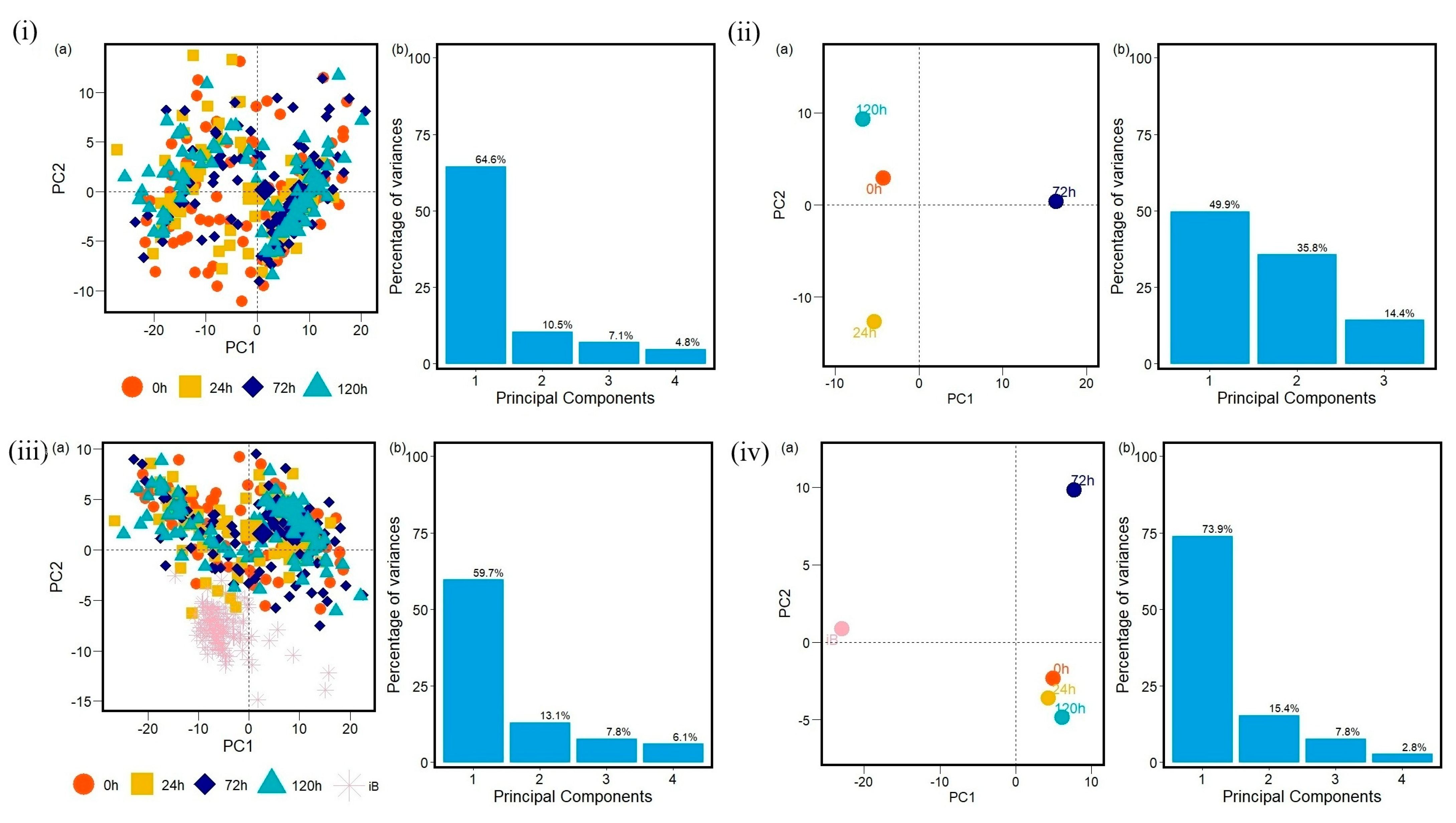
2. Results
3. Discussion
4. Materials and Methods
4.1. Samples Preparation and FTIR Spectra Acquisition
4.1.1. Resistance Induction
4.1.2. Minimum Inhibitory Concentration
4.1.3. Fourier Transformation Infrared (FTIR) Spectra Acquisition
4.2. Methodology and Machine Learning Algorithms
4.2.1. Machine Learning—Data Processing
4.2.2. Machine Learning—Hierarchical Clustering
4.2.3. Machine Learning—Principal Component Analysis
5. Conclusions
Supplementary Materials
Author Contributions
Funding
Institutional Review Board Statement
Informed Consent Statement
Data Availability Statement
Conflicts of Interest
References
- Cantón, R.; Morosini, M.-I. Emergence and Spread of Antibiotic Resistance Following Exposure to Antibiotics. FEMS Microbiol. Rev. 2011, 35, 977–991. [Google Scholar] [CrossRef] [PubMed]
- Reygaert, W.C. An Overview of the Antimicrobial Resistance Mechanisms of Bacteria. AIMS Microbiol. 2018, 4, 482–501. [Google Scholar] [CrossRef] [PubMed]
- Magréault, S.; Jauréguy, F.; Carbonnelle, E.; Zahar, J.-R. When and How to Use MIC in Clinical Practice? Antibiotics 2022, 11, 1748. [Google Scholar] [CrossRef] [PubMed]
- Kowalska-Krochmal, B.; Dudek-Wicher, R. The Minimum Inhibitory Concentration of Antibiotics: Methods, Interpretation, Clinical Relevance. Pathogens 2021, 10, 165. [Google Scholar] [CrossRef] [PubMed]
- World Health Organization. Ten Threats to Global Health in 2019; World Health Organization: Geneva, Switzerland, 2019. [Google Scholar]
- World Health Organization. Antimicrobial Resistance: Global Report on Surveillance; World Health Organization: Geneva, Switzerland, 2014; ISBN 9789241564748. [Google Scholar]
- Antimicrobial Resistance Division (AMR). A One Health Priority Research Agenda for Antimicrobial Resistance; World Health Organization: Geneva, Switzerland, 2023; ISBN 978-92-4-007592-4. [Google Scholar]
- Antimicrobial Resistance Division (AMR). WHO Strategic Priorities on Antimicrobial Resistance; World Health Organization: Geneva, Switzerland, 2022; ISBN 9789240041387. [Google Scholar]
- Prestinaci, F.; Pezzotti, P.; Pantosti, A. Antimicrobial Resistance: A Global Multifaceted Phenomenon. Pathog. Glob. Health 2015, 109, 309–318. [Google Scholar] [CrossRef] [PubMed]
- Gould, I.M. The Epidemiology of Antibiotic Resistance. Int. J. Antimicrob. Agents 2008, 32, S2–S9. [Google Scholar] [CrossRef] [PubMed]
- Harbarth, S.; Balkhy, H.H.; Goossens, H.; Jarlier, V.; Kluytmans, J.; Laxminarayan, R.; Saam, M.; Van Belkum, A.; Pittet, D. Antimicrobial Resistance: One World, One Fight! Antimicrob. Resist. Infect. Control 2015, 4, 49. [Google Scholar] [CrossRef]
- Paphitou, N.I. Antimicrobial Resistance: Action to Combat the Rising Microbial Challenges. Int. J. Antimicrob. Agents 2013, 42, S25–S28. [Google Scholar] [CrossRef] [PubMed]
- Ben, Y.; Fu, C.; Hu, M.; Liu, L.; Wong, M.; Zheng, C. Human Health Risk Assessment of Antibiotic Resistance Associated with Antibiotic Residues in the Environment: A Review. Environ. Res. 2019, 169, 483–493. [Google Scholar] [CrossRef] [PubMed]
- Mancuso, G.; Midiri, A.; Gerace, E.; Biondo, C. Bacterial Antibiotic Resistance: The Most Critical Pathogens. Pathogens 2021, 10, 1310. [Google Scholar] [CrossRef] [PubMed]
- Subramaniam, G.; Girish, M. Antibiotic Resistance—A Cause for Reemergence of Infections. Indian J. Pediatr. 2020, 87, 937–944. [Google Scholar] [CrossRef] [PubMed]
- English, B.K.; Gaur, A.H. The Use and Abuse of Antibiotics and the Development of Antibiotic Resistance. In Hot Topics in Infection and Immunity in Children VI; Springer: New York, NY, USA, 2010; pp. 73–82. [Google Scholar]
- Dever, L.A. Mechanisms of Bacterial Resistance to Antibiotics. Arch. Intern. Med. 1991, 151, 886. [Google Scholar] [CrossRef] [PubMed]
- World Health Organization. Action against Antimicrobial Resistance through the Preservation of the Environment; World Health Organization: Geneva, Switzerland, 2024; p. 2. [Google Scholar]
- Wackerly, D.; Mendenhall, W.; Scheaffer, R.L. Mathematical Statistics with Applications; Cengage Learning: Boston, MA, USA, 2014. [Google Scholar]
- Levy, S.B. The Challenge of Antibiotic Resistance. Sci. Am. 1998, 278, 46–53. [Google Scholar] [CrossRef] [PubMed]
- Levy, S.B.; Marshall, B. Antibacterial Resistance Worldwide: Causes, Challenges and Responses. Nat. Med. 2004, 10, S122–S129. [Google Scholar] [CrossRef] [PubMed]
- Slama, T.G. Gram-Negative Antibiotic Resistance: There Is a Price to Pay. Crit. Care 2008, 12, S4. [Google Scholar] [CrossRef] [PubMed]
- Dadgostar, P. Antimicrobial Resistance: Implications and Costs. Infect. Drug Resist. 2019, 12, 3903–3910. [Google Scholar] [CrossRef] [PubMed]
- Uysal Ciloglu, F.; Saridag, A.M.; Kilic, I.H.; Tokmakci, M.; Kahraman, M.; Aydin, O. Identification of Methicillin-Resistant: Staphylococcus Aureus Bacteria Using Surface-Enhanced Raman Spectroscopy and Machine Learning Techniques. Analyst 2020, 145, 7559–7570. [Google Scholar] [CrossRef] [PubMed]
- Chahine, E.B.; Dougherty, J.A.; Thornby, K.-A.; Guirguis, E.H. Antibiotic Approvals in the Last Decade: Are We Keeping Up With Resistance? Ann. Pharmacother. 2022, 56, 441–462. [Google Scholar] [CrossRef] [PubMed]
- Exner, M.; Bhattacharya, S.; Christiansen, B.; Gebel, J.; Goroncy-Bermes, P.; Hartemann, P.; Heeg, P.; Ilschner, C.; Kramer, A.; Larson, E.; et al. Antibiotic Resistance: What Is so Special about Multidrug-Resistant Gram-Negative Bacteria ? Antibiotikaresistenz: Was Ist so Besonders an Den Gram-Negativen. GMS Hyg. Infect. Control 2017, 12, Doc05. [Google Scholar] [PubMed]
- Blair, J.M.A.; Webber, M.A.; Baylay, A.J.; Ogbolu, D.O.; Piddock, L.J.V. Molecular Mechanisms of Antibiotic Resistance. Nat. Rev. Microbiol. 2015, 13, 42–51. [Google Scholar] [CrossRef] [PubMed]
- Egorov, A.M.; Ulyashova, M.M.; Rubtsova, M.Y. Microbial Enzyme Production. J. Ferment. Technol. 1988, 66, 365–366. [Google Scholar] [CrossRef]
- Talebi Bezmin Abadi, A.; Rizvanov, A.A.; Haertlé, T.; Blatt, N.L. World Health Organization Report: Current Crisis of Antibiotic Resistance. Bionanoscience 2019, 9, 778–788. [Google Scholar] [CrossRef]
- Peterson, E.; Kaur, P. Antibiotic Resistance Mechanisms in Bacteria: Relationships Between Resistance Determinants of Antibiotic Producers, Environmental Bacteria, and Clinical Pathogens. Front. Microbiol. 2018, 9, 2928. [Google Scholar] [CrossRef] [PubMed]
- Willis, J.A.; Cheburkanov, V.; Chen, S.; Soares, J.M.; Kassab, G.; Blanco, K.C.; Bagnato, V.S.; de Figueiredo, P.; Yakovlev, V.V. Breaking down Antibiotic Resistance in Methicillin-Resistant Staphylococcus aureus: Combining Antimicrobial Photodynamic and Antibiotic Treatments. Proc. Natl. Acad. Sci. USA 2022, 119, e2208378119. [Google Scholar] [CrossRef] [PubMed]
- Barrera-Patiño, C.P.; Soares, J.M.; Branco, K.C.; Inada, N.M.; Bagnato, V.S. Spectroscopic Identification of Bacteria Resistance to Antibiotics by Means of Absorption of Specific Biochemical Groups and Special Machine Learning Algorithm. Antibiotics 2023, 12, 1502. [Google Scholar] [CrossRef] [PubMed]
- Soares, J.M.; Guimarães, F.E.G.; Yakovlev, V.V.; Bagnato, V.S.; Blanco, K.C. Physicochemical Mechanisms of Bacterial Response in the Photodynamic Potentiation of Antibiotic Effects. Sci. Rep. 2022, 12, 21146. [Google Scholar] [CrossRef] [PubMed]
- Soares, J.M.; Yakovlev, V.V.; Blanco, K.C.; Bagnato, V.S. Recovering the Susceptibility of Antibiotic-Resistant Bacteria Using Photooxidative Damage. Proc. Natl. Acad. Sci. USA 2023, 120, e2311667120. [Google Scholar] [CrossRef] [PubMed]
- Barrera Patiño, C.P.; Soares, J.M.; Blanco, K.C.; Bagnato, V.S. Machine Learning in FTIR Spectrum for the Identification of Antibiotic Resistance: A Demonstration with Different Species of Microorganisms. Antibiotics 2024, 13, 821. [Google Scholar] [CrossRef] [PubMed]
- The MathWorks Inc. MATLAB R2021b. 2021. Available online: https://www.mathworks.com (accessed on 17 June 2025).
- Nguyen, G.; Dlugolinsky, S.; Bobák, M.; Tran, V.; López García, Á.; Heredia, I.; Malík, P.; Hluchý, L. Machine Learning and Deep Learning Frameworks and Libraries for Large-Scale Data Mining: A Survey. Artif. Intell. Rev. 2019, 52, 77–124. [Google Scholar] [CrossRef]
- Rizzo, M.L. Statistical Computing with R; CRC Press: Boca Raton, FL, USA, 2019. [Google Scholar]
- R Core Team. R: A Language and Environment for Statistical Computing; R Core Team: Vienna, Austria, 2021. [Google Scholar]
- R Core Team. R: A Language and Environment for Statistical Computing; R Core Team: Vienna, Austria, 2013. [Google Scholar]
- Mair, P.; Hofmann, E.; Gruber, K.; Hatzinger, R.; Zeileis, A.; Hornik, K. Motivation, Values, and Work Design as Drivers of Participation in the R Open Source Project for Statistical Computing. Proc. Natl. Acad. Sci. USA 2015, 112, 14788–14792. [Google Scholar] [CrossRef] [PubMed]
- Fox, J. Aspects of the Social Organization and Trajectory of the R Project. R J. 2009, 1, 5. [Google Scholar] [CrossRef]
- Gareth, J.; Daniela, W.; Trevor, H.; Robert, T. An Introduction to Statistical Learning: With Applications in R; Spinger: New York, NY, USA, 2013. [Google Scholar]
- Chambers, J.M. Software for Data Analysis: Programming with R; Springer: New York, UY, USA, 2008; Volume 2. [Google Scholar]
- Ripley, B.D. The R Project in Statistical Computing. MSOR Connect. Newsl. LTSN Maths, Stats OR Netw. 2001, 1, 23–25. [Google Scholar] [CrossRef]
- Python Software Foundation. Python (3.12.3). Available online: https://www.python.org/downloads/release/python-3123/ (accessed on 17 June 2025).
- Virtanen, P.; Gommers, R.; Oliphant, T.E.; Haberland, M.; Reddy, T.; Cournapeau, D.; Burovski, E.; Peterson, P.; Weckesser, W.; Bright, J.; et al. SciPy 1.0: Fundamental Algorithms for Scientific Computing in Python. Nat. Methods 2020, 17, 261–272. [Google Scholar] [CrossRef] [PubMed]
- Pedregosa, F.; Varoquaux, G.; Gramfort, A.; Michel, V.; Thirion, B.; Grisel, O.; Blondel, M.; Prettenhofer, P.; Weiss, R.; Dubourg, V.; et al. Scikit-Learn: Machine Learning in Python. J. Mach. Learn. Res. 2011, 12, 2825–2830. [Google Scholar]
- National Center for Biotechnology Information PubChem Compound Summary for CID 447043, Azithromycin. PubChem Compound Summary 2025. Available online: https://pubchem.ncbi.nlm.nih.gov/compound/447043?from=summary (accessed on 15 July 2025).
- National Center for Biotechnology Information PubChem Compound Summary for CID 6196, Oxacillin. PubChem Compound Summary 2025. Available online: https://pubchem.ncbi.nlm.nih.gov/compound/Oxacillin (accessed on 15 July 2025).
- National Center for Biotechnology Information PubChem Compound Summary for CID 5578, Trimethoprim. PubChem Compound Summary 2025. Available online: https://pubchem.ncbi.nlm.nih.gov/compound/Trimethoprim (accessed on 15 July 2025).
- Choudhury, J.; Ashraf, F.B. An Analysis of Different Distance-Linkage Methods for Clustering Gene Expression Data and Observing Pleiotropy: Empirical Study. JMIR Bioinforma. Biotechnol. 2022, 3, e30890. [Google Scholar] [CrossRef] [PubMed]
- Cabral, D.; Wurster, J.; Belenky, P. Antibiotic Persistence as a Metabolic Adaptation: Stress, Metabolism, the Host, and New Directions. Pharmaceuticals 2018, 11, 14. [Google Scholar] [CrossRef] [PubMed]
- Uddin, T.M.; Chakraborty, A.J.; Khusro, A.; Zidan, B.R.M.; Mitra, S.; Emran, T.B.; Dhama, K.; Ripon, M.K.H.; Gajdács, M.; Sahibzada, M.U.K.; et al. Antibiotic Resistance in Microbes: History, Mechanisms, Therapeutic Strategies and Future Prospects. J. Infect. Public Health 2021, 14, 1750–1766. [Google Scholar] [CrossRef] [PubMed]
- Vijaya; Sharma, S.; Batra, N. Comparative Study of Single Linkage, Complete Linkage, and Ward Method of Agglomerative Clustering. In Proceedings of the 2019 International Conference on Machine Learning, Big Data, Cloud and Parallel Computing (COMITCon), Faridabad, India, 14–16 February 2019; pp. 568–573. [Google Scholar]


| Antibiotic | Chemical Structure | Properties |
|---|---|---|
| Azithromycin (Azy) C38H72N2O12 [36] | 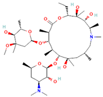 | In order to replicate, bacteria require a specific process of protein synthesis enabled by ribosomal proteins. Azithromycin binds to the 23S rRNA of the bacterial 50S ribosomal subunit. It stops bacterial protein synthesis by inhibiting the transpeptidation/translocation step of protein synthesis and by inhibiting the assembly of the 50S ribosomal subunit. Azithromycin is highly stable at a low pH, giving it a longer serum half-life and increasing its concentrations in tissues compared to erythromycin [36]. |
| Oxacillin (Oxa) C19H19N3O5S [37] | 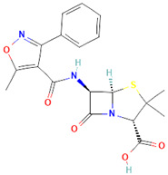 | By binding to specific penicillin-binding proteins (PBPs) located inside the bacterial cell wall, Oxacillin inhibits the third and last stage of bacterial cell wall synthesis. Cell lysis is then mediated by bacterial cell wall autolytic enzymes such as autolysins; it is possible that Oxacillin interferes with an autolysin inhibitor [37]. |
| Trimethoprim/Sulfamethoxazole (Trim) C14H18N4O3 [38] |  | Trimethoprim is a reversible inhibitor of dihydrofolate reductase, one of the principal enzymes catalyzing the formation of tetrahydrofolic acid (THF) from dihydrofolic acid (DHF). Tetrahydrofolic acid is necessary for the biosynthesis of bacterial nucleic acids and proteins and ultimately for continued bacterial survival—inhibiting its synthesis, which then results in bactericidal activity. Trimethoprim is often given in combination with sulfamethoxazole, which inhibits the preceding step in bacterial protein synthesis. Given together, sulfamethoxazole and trimethoprim inhibit two consecutive steps in the biosynthesis of bacterial nucleic acids and proteins [38]. |
Disclaimer/Publisher’s Note: The statements, opinions and data contained in all publications are solely those of the individual author(s) and contributor(s) and not of MDPI and/or the editor(s). MDPI and/or the editor(s) disclaim responsibility for any injury to people or property resulting from any ideas, methods, instructions or products referred to in the content. |
© 2025 by the authors. Licensee MDPI, Basel, Switzerland. This article is an open access article distributed under the terms and conditions of the Creative Commons Attribution (CC BY) license (https://creativecommons.org/licenses/by/4.0/).
Share and Cite
Barrera Patiño, C.P.; Bonner, M.; Borsatto, A.R.; Soares, J.M.; Blanco, K.C.; Bagnato, V.S. Time Evolution of Bacterial Resistance Observed with Principal Component Analysis. Antibiotics 2025, 14, 729. https://doi.org/10.3390/antibiotics14070729
Barrera Patiño CP, Bonner M, Borsatto AR, Soares JM, Blanco KC, Bagnato VS. Time Evolution of Bacterial Resistance Observed with Principal Component Analysis. Antibiotics. 2025; 14(7):729. https://doi.org/10.3390/antibiotics14070729
Chicago/Turabian StyleBarrera Patiño, Claudia P., Mitchell Bonner, Andrew Ramos Borsatto, Jennifer M. Soares, Kate C. Blanco, and Vanderlei S. Bagnato. 2025. "Time Evolution of Bacterial Resistance Observed with Principal Component Analysis" Antibiotics 14, no. 7: 729. https://doi.org/10.3390/antibiotics14070729
APA StyleBarrera Patiño, C. P., Bonner, M., Borsatto, A. R., Soares, J. M., Blanco, K. C., & Bagnato, V. S. (2025). Time Evolution of Bacterial Resistance Observed with Principal Component Analysis. Antibiotics, 14(7), 729. https://doi.org/10.3390/antibiotics14070729