Figure 1.
The positive background density for in the step-like and smooth density profile models.
Figure 1.
The positive background density for in the step-like and smooth density profile models.
Figure 2.
The potential energies (
19) and (
20) of the positive background with the density profiles (
11) and (
13) for
.
Figure 2.
The potential energies (
19) and (
20) of the positive background with the density profiles (
11) and (
13) for
.
Figure 3.
Configurations of the Wigner crystal molecules with
in the field of the positively charged background with the step-like density (
11). The white circle shows the boundary of the positively charged disk; the length unit is
. For
, the single-shell configurations (
a–
d) have a lower energy. For
, the two-shell configurations (
g,
h) have a lower energy. For
, the energies of the single-shell (
e) and the two-shell (
f) configurations are very close.
Figure 4.
The energy per particle of the Wigner crystal molecules in the N-electron systems with the and configurations for (a) the step-like and (b) smooth density profiles.
Figure 4.
The energy per particle of the Wigner crystal molecules in the N-electron systems with the and configurations for (a) the step-like and (b) smooth density profiles.
Figure 5.
The energy per particle of the exact ground (black circles) and the first excited (red squares) states, Equation (
69), as well as of the Laughlin state (
5), at
, as a function of the number of particles
N. The energies are in units
.
Figure 5.
The energy per particle of the exact ground (black circles) and the first excited (red squares) states, Equation (
69), as well as of the Laughlin state (
5), at
, as a function of the number of particles
N. The energies are in units
.
Figure 6.
(
a) The density of electrons in the exact ground state (thick solid curves), together with the density of the positive background (thin dashed curves) for
for the step-like background density profile (
11). Arrows above the curves show the radii of the outer shells
of the Wigner molecules, see
Table 3; for
, the shell radii of both
(dashed arrow) and
(solid arrow) configurations are shown. (
b) The density of electrons in the exact ground state (
) and the first excited state (
) for
.
Figure 7.
The pair correlation function
in the ground state, as a function of
and
, for different
N and different coordinates
: (
a)
and
; (
b)
and
; (
c)
and
; and (
d)
and
. The positions of the
points are shown by small black circles; in (
a–
c), they correspond to the maxima of the electron density, see
Figure 6.
Figure 8.
The energy per particle of the MDD state (
72), measured in units
, (
a) as a function of the number of electrons
N and (
b) as a function of
. The red arrow in (
a) and red point in (
b) show the asymptotic value (
82), reported in Ref. [
6].
Figure 8.
The energy per particle of the MDD state (
72), measured in units
, (
a) as a function of the number of electrons
N and (
b) as a function of
. The red arrow in (
a) and red point in (
b) show the asymptotic value (
82), reported in Ref. [
6].
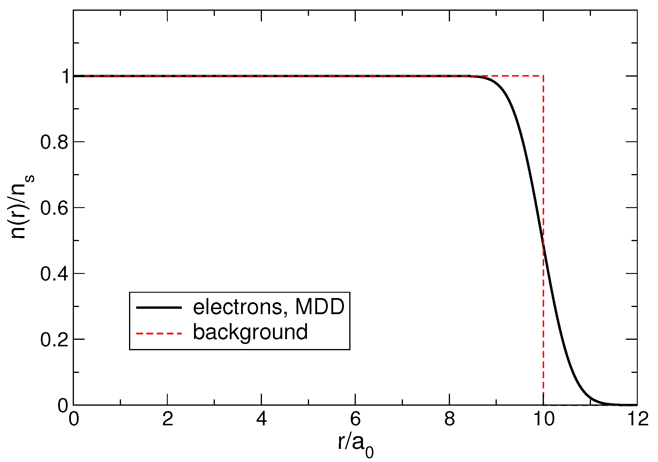
Figure 9.
The density of the electrons in the MDD state at (black solid curve) and the density of the positive background (red dashed curve) for . The density is plotted as a function of or (at ).
Figure 9.
The density of the electrons in the MDD state at (black solid curve) and the density of the positive background (red dashed curve) for . The density is plotted as a function of or (at ).
Figure 10.
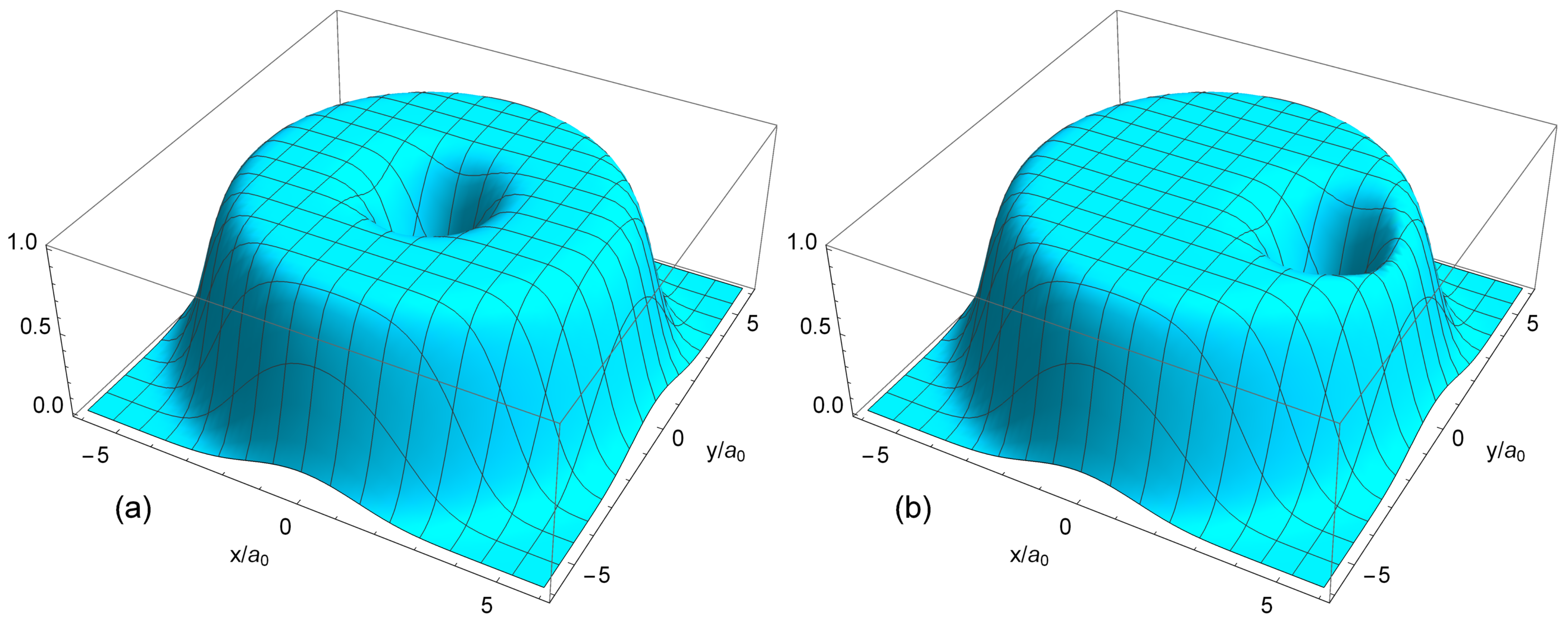
The pair correlation function of the MDD state (
72), as a function of
, at
and (
a)
and (
b)
.
Figure 10.
The pair correlation function of the MDD state (
72), as a function of
, at
and (
a)
and (
b)
.
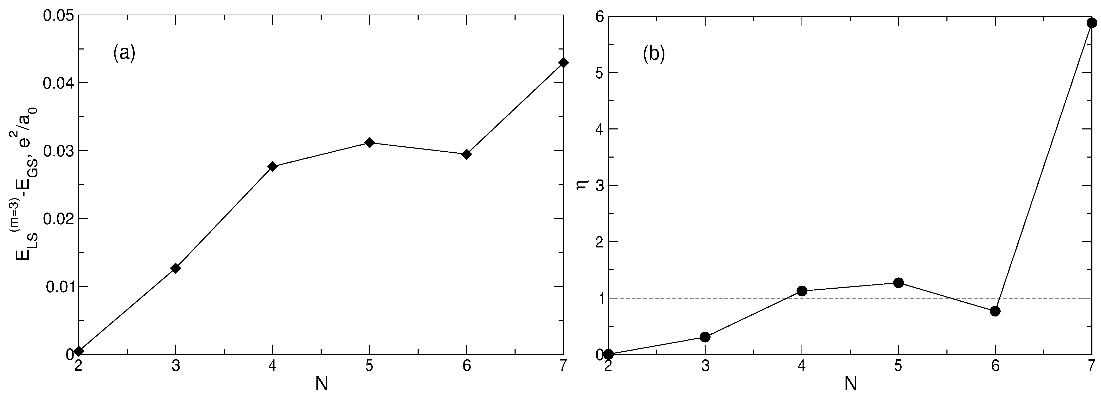
Figure 11.
(
a) The energy difference
between the Laughlin state and the true ground state of a system of
N particles as a function of
N; the energy unit is
. (
b) The value of
defined by Equation (
97), as a function of
N.
Figure 11.
(
a) The energy difference
between the Laughlin state and the true ground state of a system of
N particles as a function of
N; the energy unit is
. (
b) The value of
defined by Equation (
97), as a function of
N.
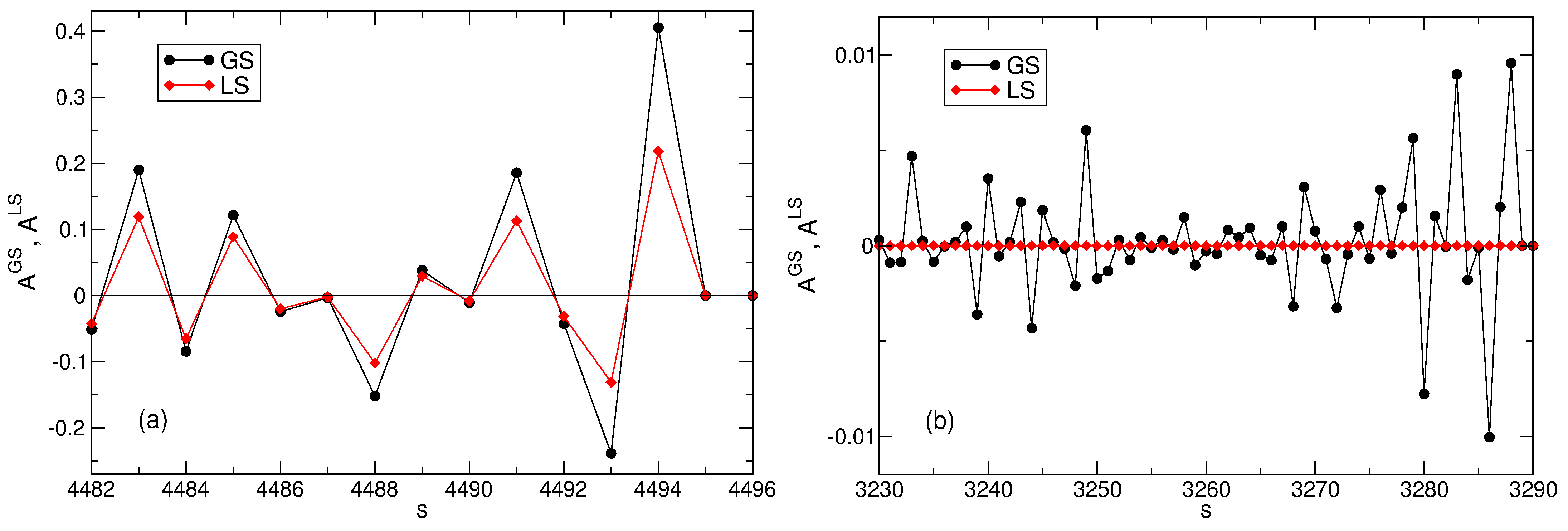
Figure 12.
The expansion coefficients
and
of the true ground state wave function (
58) and of the Laughlin state (
84) for a few selected many-body basis states: (
a)
and (
b)
. The Landau level filling factor is
, the number of particles is
, the total angular momentum is
, and the total number of many-body basis states is
.
Figure 13.
(
a) The density of electrons
(solid curves) in the Laughlin state (
5) at
, as a function of the radial coordinate for
–8. The dashed lines show the corresponding positive background densities; the thin horizontal black line indicates the level 0.5, which determines the radii of the electron disks. (
b) The absolute value of the density difference between the true ground state and the LS for different
N. (
c) The density of electrons in the true ground state (GS) and the Laughlin state (LS) at
.
Figure 14.
The pair correlation functions for the exact ground state (GS) and the Laughlin state (LS), for a system of particles.
Figure 14.
The pair correlation functions for the exact ground state (GS) and the Laughlin state (LS), for a system of particles.
Figure 15.
The density of electrons in the MDD, MDD-plus, and MDD-shift states as a function of for .
Figure 15.
The density of electrons in the MDD, MDD-plus, and MDD-shift states as a function of for .
Figure 16.
(a) The energy of the MDD, MDD-plus, and MDD-shift states, as a function of . (b) The energy differences as a function of .
Figure 16.
(a) The energy of the MDD, MDD-plus, and MDD-shift states, as a function of . (b) The energy differences as a function of .
Figure 17.
The coordinate dependencies of the density of electrons in the Laughlin states (
5) at
,
, and
, calculated for
by Ciftja et al. in Refs. [
23,
24]; the discrete numerical data points are connected by lines to guide the eye. The thick black solid curve shows the MDD density at
. At
(not shown in the Figure), the normalized electron density equals 1 according to Refs. [
23,
24]. A thin horizontal line at the level of 0.5 visualizes the change of the electron disk radius when
decreases from
to
.
Figure 18.
Fitting of the numerical data [
23] for the density of electrons in the
LS by the analytical function (
104) for (
a)
; (
b)
; (
c)
; and (
d)
.
Figure 18.
Fitting of the numerical data [
23] for the density of electrons in the
LS by the analytical function (
104) for (
a)
; (
b)
; (
c)
; and (
d)
.
Figure 19.
The density of electrons in the MDD (
) and in the Laughlin states (
5) with
,
, and
. The number of particles is
. The data for the Laughlin electron densities are taken from Refs. [
23,
24].
Figure 19.
The density of electrons in the MDD (
) and in the Laughlin states (
5) with
,
, and
. The number of particles is
. The data for the Laughlin electron densities are taken from Refs. [
23,
24].
Figure 20.
(a) The energy of the many-body states with the total angular momenta from up to in the system of 2D electrons as a function of the magnetic field parameter . The index s enumerates different states with the same . The LS energy at is shown by a small red circle. (b) The energy gap between the ground and the first excited states as a function of . The positive background density profile is step-like.
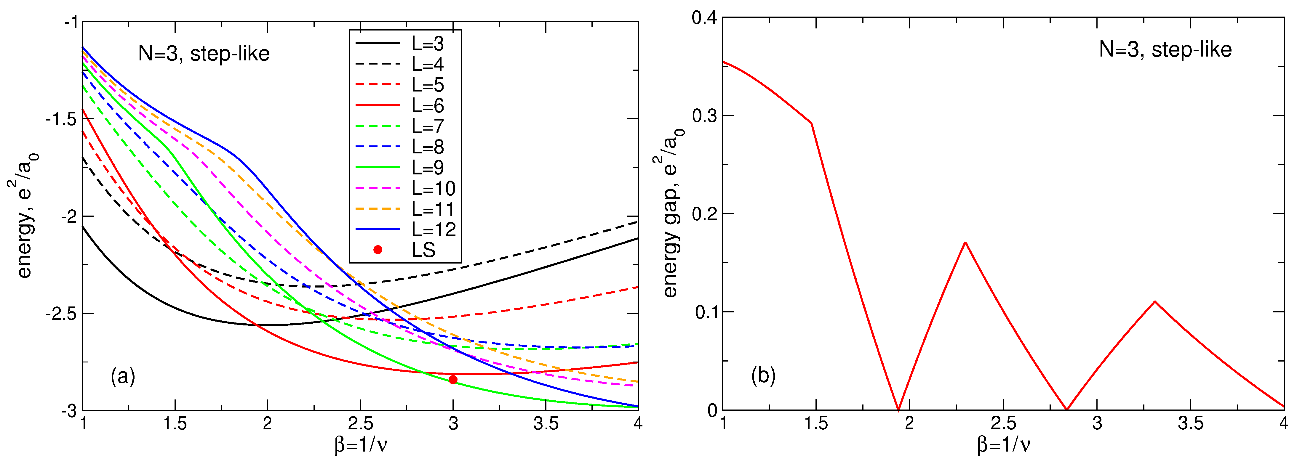
Figure 21.
(a) The energy of the many-body states with the total angular momenta from up to in the system of 2D electrons as a function of the magnetic field parameter . For all shown states, the index s equals ; the states with are not shown. The LS energy at is shown by a small red circle. (b) The energy gap between the ground and the first excited states as a function of . The positive background density profile is step-like.
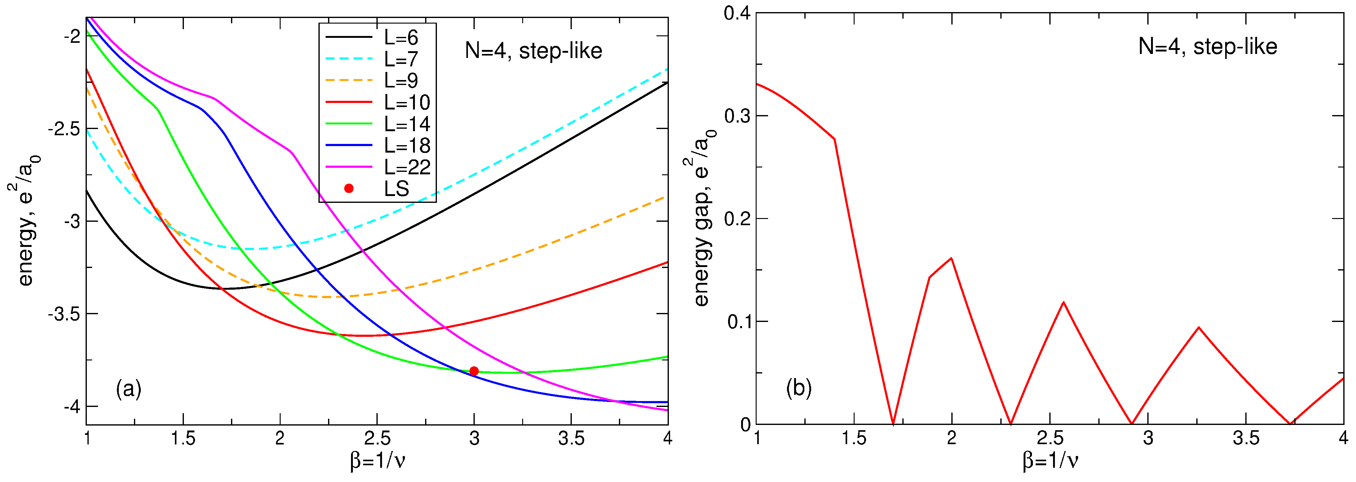
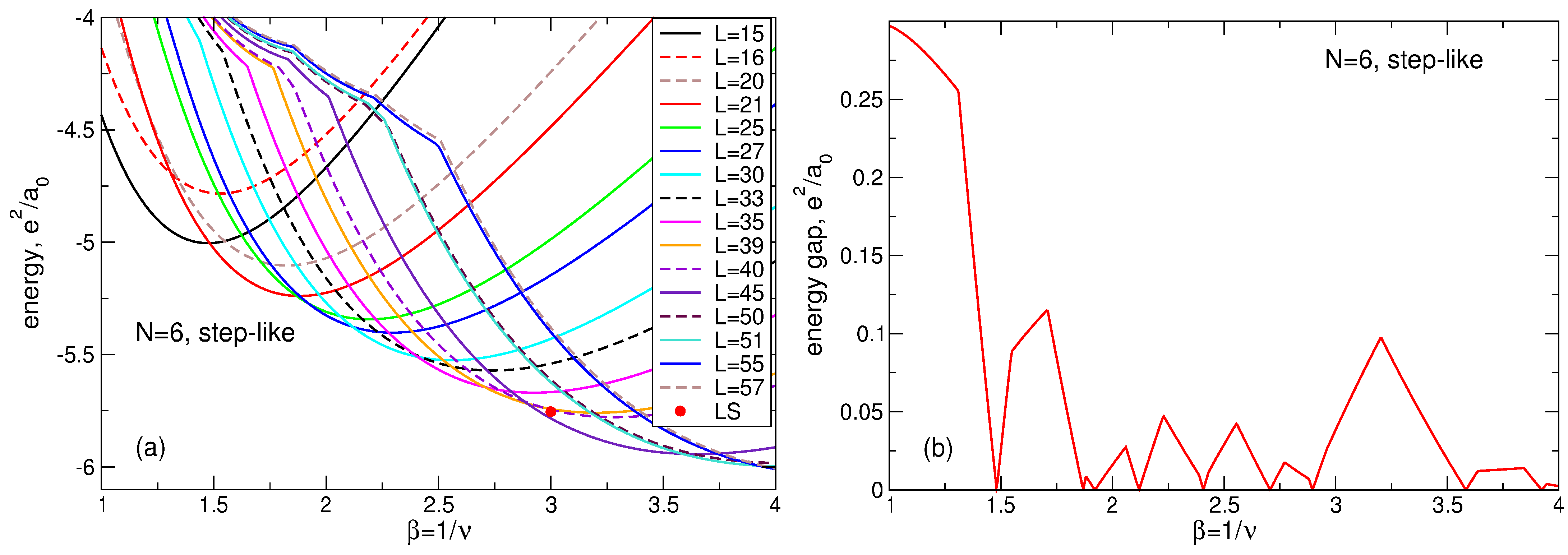
Figure 22.
(a) The energy of the many-body states with the total angular momenta from up to in the system of 2D electrons as a function of the magnetic field parameter . For all shown states, the index s equals . Only the states which are either ground or first excited states are shown. The LS energy at is shown by a small red circle. (b) The energy gap between the ground and the first excited states as a function of . The positive background density profile is step-like.
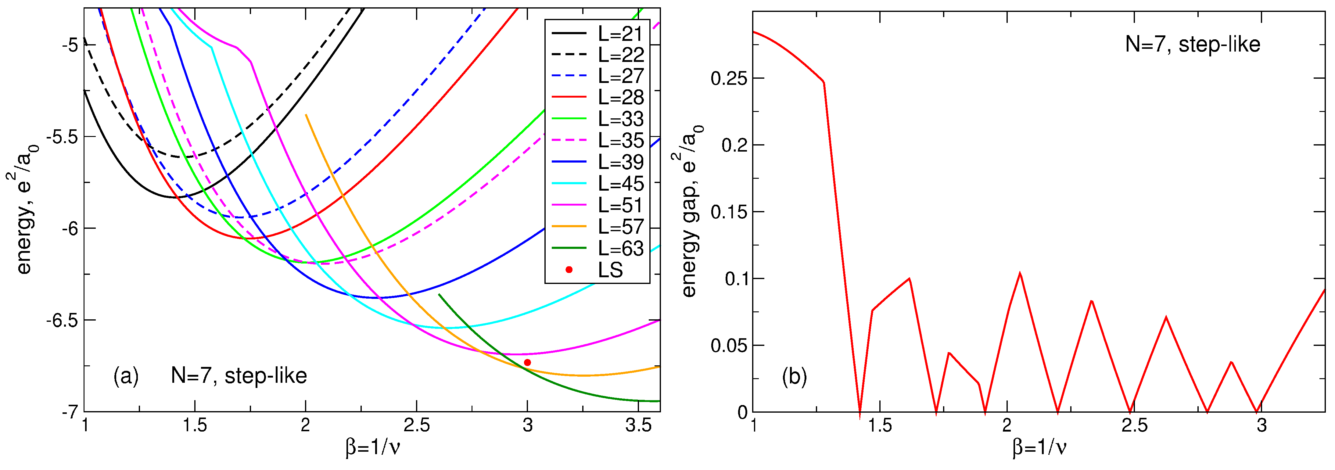
Figure 23.
(a) The energy of the many-body states with the total angular momenta from up to in the system of 2D electrons as a function of the magnetic field parameter . For all shown states, the index s equals . Only the states which are either ground or first excited states are shown. The LS energy at is shown by a small red circle. (b) The energy gap between the ground and the first excited states as a function of . The positive background density profile is step-like.
Figure 24.
(a) The energy of the many-body states with the total angular momenta from up to in the system of 2D electrons as a function of the magnetic field parameter . For all shown states, the index s equals . Only the states which are either ground or first excited states are shown. The LS energy at is shown by a small red circle. (b) The energy gap between the ground and the first excited states as a function of . The positive background density profile is step-like.
Figure 25.
(a) The energy of the many-body states with the total angular momenta from up to in the system of 2D electrons as a function of the magnetic field parameter . For all shown states, the index s equals . Only the states which are either ground or first excited states are shown. The LS energy at is shown by a small red circle. (b) The energy gap between the ground and the first excited states as a function of . The positive background density profile is step-like.
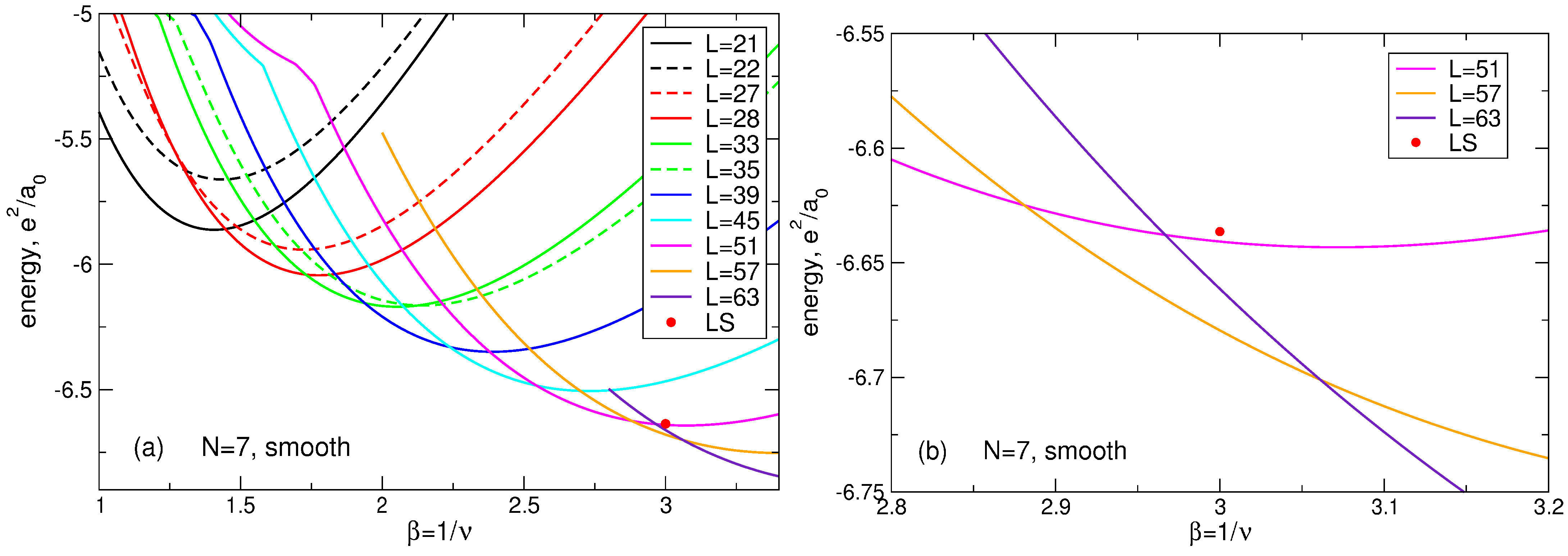
Figure 26.
(a) The energy of the many-body states with the total angular momenta from up to in the system of 2D electrons as a function of the magnetic field parameter . For all shown states, the index s equals . Only the states which are either ground or first excited states are shown. The LS energy at is shown by a small red circle. (b) The vicinity of the point on a larger scale. The positive background density profile is smooth.
Figure 27.
The density of electrons in the system of particles at different magnetic fields and at (a) and (b) . For -values, for which the corresponding state is the ground state (one of the excited states), the function is shown by solid (dashed) curves. The vertical arrow at shows the position of the shell radius in the classical Wigner molecule. The positive background density profile is step-like and shown by the black dotted curve in both panels.
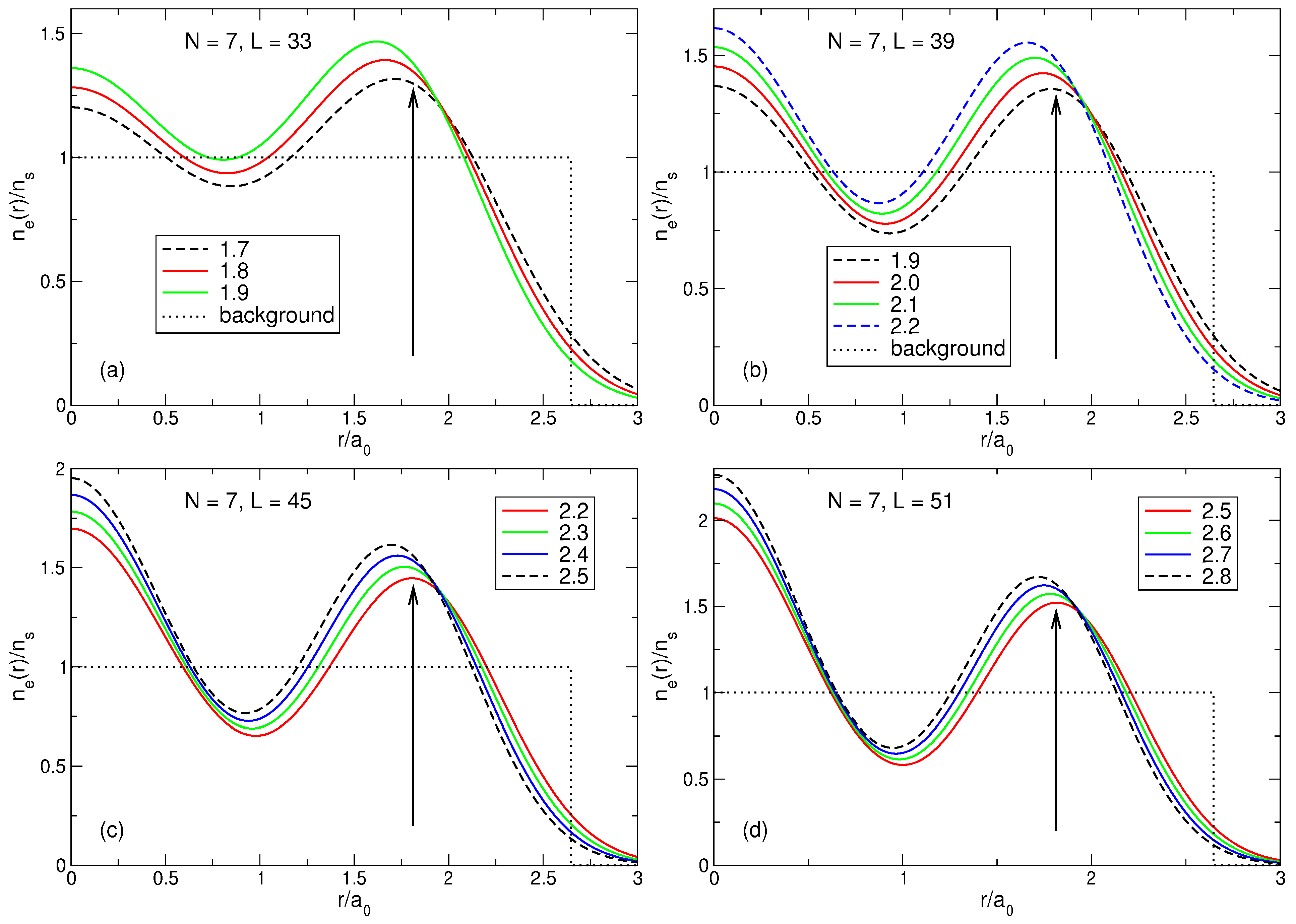
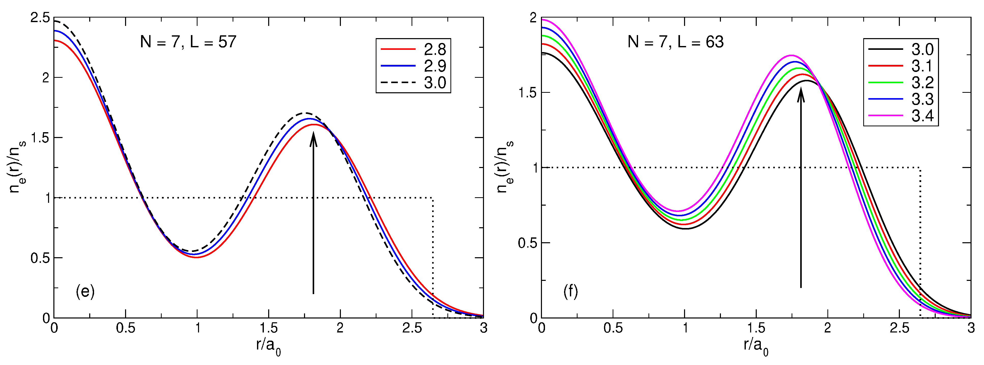
Figure 28.
The density of electrons in the system of particles at different magnetic fields and at (a) , (b) , (c) , (d) , (e) , and (f) . For -values, for which the corresponding state is the ground state, the function is shown by solid curves. The arrow at shows the position of the shell radius in the classical Wigner molecule. The step-like positive background density profile is shown by the black dotted curve in all panels.
Figure 29.
Positions of the maxima of the density curves shown in
Figure 28 at different
-values and different angular momenta
. The red dashed line at
shows the position of the shell radius in the classical Wigner molecule. The blue dash-dotted lines separate the areas where the ground states have different angular momenta indicated by the numbers 33, 39, …, 63 in the corresponding
-intervals.
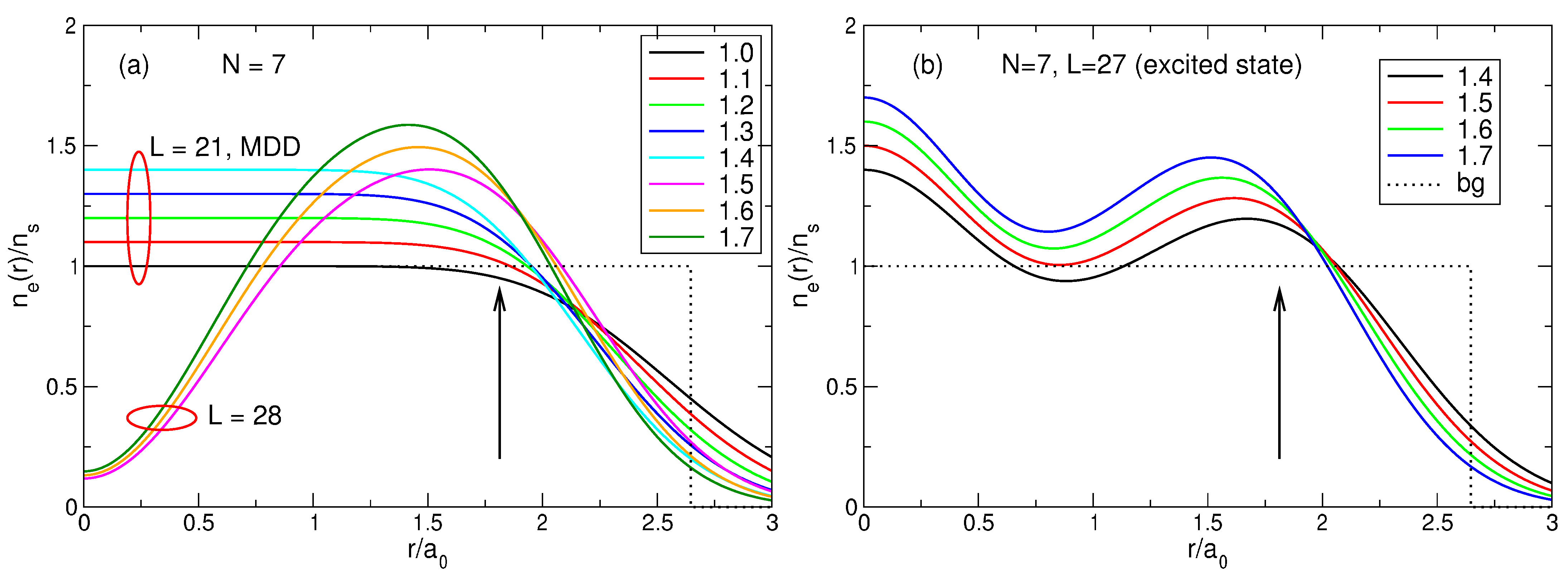
Figure 30.
The density of electrons in the system of particles at different magnetic fields and (a) in the ground states with and 28, and (b) in the excited state with . The arrow at shows the position of the shell radius in the classical Wigner molecule. The step-like positive background density profile is shown by the black dotted curve in both panels.
Figure 31.
The density of electrons in the ground state (), first () and second () excited states, and in the LS in a system of particles at . The positive background density profile is smooth. The arrow at shows the position of the outer shell of the classical Wigner molecule in the case of the smooth background density. The density of the LS at is 2.2576 times smaller than the density of the ground state.
Figure 32.
(
a) The energy of the Laughlin state and the Laughlin excitations (“quasiholes” and “quasielectrons”), together with the energies of the exact ground and excited states in the vicinity of the filling factor
. The green (blue) thin curves show the energy of the
(
) exact excited states with different
; not all exact excited states with energies lower than the energy of the Laughlin “quasihole” are shown. (
b) The density of electrons in the Laughlin “quasiholes” and “quasielectrons” states (
122) and (
123).
Figure 33.
The Coulomb interaction potential (black curve) and the potential (
132). The energy is in units
. Inset shows a sphere with two interacting electrons
A and
B separated by a polar angle
.
Figure 33.
The Coulomb interaction potential (black curve) and the potential (
132). The energy is in units
. Inset shows a sphere with two interacting electrons
A and
B separated by a polar angle
.
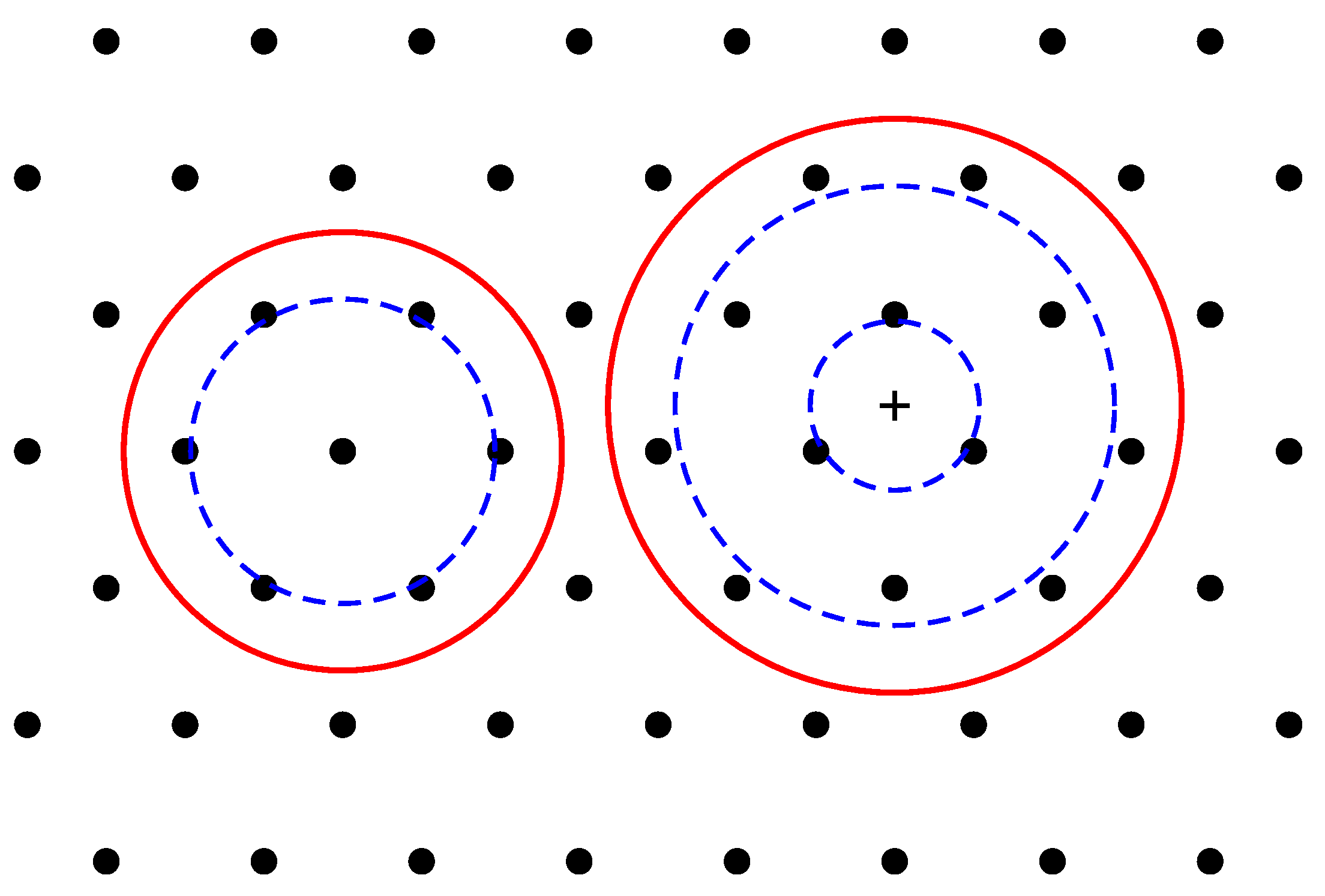
Figure 34.
Wigner crystal fragments of the macroscopic lattice with
and
electrons. The red circles show the boundaries of the disks containing
N electrons, and the blue dashed circles correspond to the maxima of the electron density calculated in [
19]. The common center of all 12 electrons is shown by a small cross in the right part of the figure.
Table 1.
Possible many-body configurations in a system of electrons. is the total number of all many-particle configurations with a given N and .
Table 1.
Possible many-body configurations in a system of electrons. is the total number of all many-particle configurations with a given N and .
| Configurations | |
|---|
| 1 | | 1 |
| 2 | | 1 |
| 3 |
| 2 |
| 4 |
| 2 |
| 5 |
| 3 |
| 6 |
| 3 |
| 7 |
| 4 |
Table 2.
Possible many-body configurations in a system of particles. is the total number of all many-particle configurations with given N and .
Table 2.
Possible many-body configurations in a system of particles. is the total number of all many-particle configurations with given N and .
| Configurations | |
|---|
| 3 | | 1 |
| 4 | | 1 |
| 5 |
| 2 |
| 6 |
| 3 |
| 7 |
| 4 |
| 8 |
| 5 |
| 9 |
| 7 |
| 10 |
| 8 |
| 11 |
| 10 |
| 12 |
| 12 |
Table 3.
Parameters of the Wigner molecules in one-shell
and two-shell
configurations for the step-like density profile (
11) and
.
R is the radius of the positively charged background disk, and
are the radii of the shells obtained by the minimization of the energies (
61) and (
64).
and
are the Wigner molecule energies per particle for two configurations. The lengths are in units
, and the energies are in units
.
| N | R | Configuration | | | Configuration | | |
|---|
| 2 | | (0, 2) | 0.684302 | | | | |
| 3 | | (0, 3) | 0.956542 | | (1, 2) | 1.196868 | |
| 4 | | (0, 4) | 1.178838 | | (1, 3) | 1.361107 | |
| 5 | | (0, 5) | 1.373422 | | (1, 4) | 1.518623 | |
| 6 | | (0, 6) | 1.549288 | | (1, 5) | 1.669034 | |
| 7 | | (0, 7) | 1.711287 | | (1, 6) | 1.812600 | |
| 8 | | (0, 8) | 1.862429 | | (1, 7) | 1.949843 | |
Table 4.
The same as in
Table 3 but for the smooth density profile (
13).
Table 4.
The same as in
Table 3 but for the smooth density profile (
13).
| N | R | Configuration | | | Configuration | | |
|---|
| 2 | | (0, 2) | 0.621826 | | | | |
| 3 | | (0, 3) | 0.888015 | | (1, 2) | 1.127002 | |
| 4 | | (0, 4) | 1.107700 | | (1, 3) | 1.282076 | |
| 5 | | (0, 5) | 1.301195 | | (1, 4) | 1.437241 | |
| 6 | | (0, 6) | 1.476787 | | (1, 5) | 1.587616 | |
| 7 | | (0, 7) | 1.638979 | | (1, 6) | 1.732047 | |
| 8 | | (0, 8) | 1.790593 | | (1, 7) | 1.870522 | |
Table 5.
Exact and Laughlin energies, as well as relevant angular momenta, of the lowest-energy states for the different numbers of particles
N. Second column: The total angular momentum
corresponding to the true ground and Laughlin states. Third and fourth columns: The exact energies of the two lowest levels of the states with
. Fifth and sixth columns: The total angular momentum
and the lowest energy
corresponding to the true first excited state; here
, Equation (
65). Seventh column: The energy difference
between the true first excited and the true ground state, as shown in Equation (
69). Eighth column: The exactly calculated energy of the Laughlin state. Ninth column: The energy difference
between the LS and the true ground state. All energies are in units
. The step-like background density profile is assumed.
| N | | | | | | | | |
|---|
| 2 | 3 | | | 1 | | | | |
| 3 | 9 | | | 6 | | | | |
| 4 | 18 | | | 14 | | | | |
| 5 | 30 | | | 25 | | | | |
| 6 | 45 | | | 40 | | | | |
| 7 | 63 | | | 57 | | | | |
Table 6.
The expansion coefficients for the exact ground state of particles.
Table 6.
The expansion coefficients for the exact ground state of particles.
| s | State | |
|---|
| 1 | | |
| 2 | | |
Table 7.
The expansion coefficients for the exact ground state of particles.
Table 7.
The expansion coefficients for the exact ground state of particles.
| s | State | |
|---|
| 1 | | |
| 2 | | |
| 3 | | |
| 4 | | |
| 5 | | |
| 6 | | |
| 7 | | |
Table 8.
Many-body configurations for
and
, with the expansion coefficients
,
, and
. The coefficients
can be found using Equation (
92).
Table 8.
Many-body configurations for
and
, with the expansion coefficients
,
, and
. The coefficients
can be found using Equation (
92).
| No. | Configuration | | | |
|---|
| 1 | | | | |
| 2 | | 3 | | |
Table 9.
Many-body configurations for
and
, with the expansion coefficients
,
, and
. The coefficients
can be found using Equation (
92).
Table 9.
Many-body configurations for
and
, with the expansion coefficients
,
, and
. The coefficients
can be found using Equation (
92).
| No. | Configuration | | | |
|---|
| 1 | | 0 | | |
| 2 | | 0 | | |
| 3 | | | | |
| 4 | | 3 | | |
| 5 | | 3 | | |
| 6 | | | | |
| 7 | | 15 | | |
Table 10.
Many-body configurations for
and
, with the expansion coefficients
,
, and
. The coefficients
can be found using Equation (
92).
Table 10.
Many-body configurations for
and
, with the expansion coefficients
,
, and
. The coefficients
can be found using Equation (
92).
| No. | Configuration | | | |
|---|
| 15 | | 1 | | |
| 16 | | | | |
| 17 | | | | |
| 18 | | 6 | | |
| 19 | | | | |
| 23 | | | | |
| 24 | | 9 | | |
| 26 | | 6 | | |
| 27 | | | | |
| 28 | | | | |
| 29 | | 27 | | |
| 30 | | | | |
| 31 | | 27 | | |
| 32 | | | | |
| 33 | | | | |
| 34 | | 105 | | |
Table 11.
The total number of many-body states
, the number of states contributing (
) and not contributing (
) to the Laughlin function, as well as the percentage of non-contributing many-body configurations (‘% zero’).
N is the number of particles and
is the total angular momentum (
83) corresponding to
and
in Equation (
5).
| N | | | | | % Zero |
|---|
| 2 | 3 | 2 | 0 | 2 | 00.00 |
| 3 | 9 | 7 | 2 | 5 | 28.57 |
| 4 | 18 | 34 | 18 | 16 | 52.94 |
| 5 | 30 | 192 | 133 | 59 | 69.27 |
| 6 | 45 | 1206 | 959 | 247 | 79.52 |
| 7 | 63 | 8033 | 6922 | 1111 | 86.17 |
| 8 | 84 | 55974 | 50680 | 5294 | 90.54 |
Table 12.
The standard deviation (
98) and the projection (
99) of the Laughlin wave function (
5) from/onto the ground state wave function (
58) at
.
Table 12.
The standard deviation (
98) and the projection (
99) of the Laughlin wave function (
5) from/onto the ground state wave function (
58) at
.
| N | D | P |
|---|
| 2 | 0.0334 | 0.9994 |
| 3 | 0.1755 | 0.9846 |
| 4 | 0.2978 | 0.9557 |
| 5 | 0.3500 | 0.9387 |
| 6 | 0.2960 | 0.9562 |
| 7 | 0.4021 | 0.9191 |
Table 13.
The energies of the ground state, first and second excited states, as well as of the Laughlin state, at , in the case of the smooth density profile. All energies are in units .
Table 13.
The energies of the ground state, first and second excited states, as well as of the Laughlin state, at , in the case of the smooth density profile. All energies are in units .
| State | | | |
|---|
| Laughlin | 63 | −6.6363835 | 0.0431284 |
| 2nd excited | 51 | −6.6407409 | 0.0387709 |
| 1st excited | 63 | −6.6613834 | 0.0181285 |
| Ground | 57 | −6.6795119 | 0.0 |
Table 14.
The total angular momenta of the ground state and of the first excited state assume the values shown in the last two columns in the intervals from to shown in the first two columns. The number of particles is , the density profile is step-like.
Table 14.
The total angular momenta of the ground state and of the first excited state assume the values shown in the last two columns in the intervals from to shown in the first two columns. The number of particles is , the density profile is step-like.
| | | |
|---|
| 1.0000 | 1.5986 | 1 | 2 |
| 1.5986 | 2.5559 | 1 | 3 |
| 2.5559 | 3.3567 | 3 | 1 |
| 3.3567 | 4.0000 | 3 | 4 |
Table 15.
The total angular momenta of the ground state and of the first excited state assume the values shown in the last two columns in the intervals from to shown in the first two columns. The number of particles is , the density profile is step-like.
Table 15.
The total angular momenta of the ground state and of the first excited state assume the values shown in the last two columns in the intervals from to shown in the first two columns. The number of particles is , the density profile is step-like.
| | | |
|---|
| 1.0000 | 1.4751 | 3 | 4 |
| 1.4751 | 1.9397 | 3 | 6 |
| 1.9397 | 2.2971 | 6 | 3 |
| 2.2971 | 2.8392 | 6 | 9 |
| 2.8392 | 3.3096 | 9 | 6 |
| 3.3096 | 4.0000 | 9 | 12 |
Table 16.
The total angular momenta of the ground state and of the first excited state assume the values shown in the last two columns in the intervals from to shown in the first two columns. The number of particles is , and the density profile is step-like.
Table 16.
The total angular momenta of the ground state and of the first excited state assume the values shown in the last two columns in the intervals from to shown in the first two columns. The number of particles is , and the density profile is step-like.
| | | |
|---|
| 1.0000 | 1.4006 | 6 | 7 |
| 1.4006 | 1.6991 | 6 | 10 |
| 1.6991 | 1.8850 | 10 | 6 |
| 1.8850 | 1.9972 | 10 | 9 |
| 1.9972 | 2.2994 | 10 | 14 |
| 2.2994 | 2.5689 | 14 | 10 |
| 2.5689 | 2.9173 | 14 | 18 |
| 2.9173 | 3.2593 | 18 | 14 |
| 3.2593 | 3.7263 | 18 | 22 |
| 3.7263 | 4.0000 | 22 | 18 |
Table 17.
The total angular momenta of the ground state and of the first excited state assume the values shown in the last two columns in the intervals from to shown in the first two columns. The number of particles is , the density profile is step-like.
Table 17.
The total angular momenta of the ground state and of the first excited state assume the values shown in the last two columns in the intervals from to shown in the first two columns. The number of particles is , the density profile is step-like.
| | | |
|---|
| 1.0000 | 1.3483 | 10 | 11 |
| 1.3483 | 1.5666 | 10 | 15 |
| 1.5666 | 1.6688 | 15 | 10 |
| 1.6688 | 1.8486 | 15 | 14 |
| 1.8486 | 1.8647 | 15 | 18 |
| 1.8647 | 2.0402 | 15 | 20 |
| 2.0402 | 2.1372 | 20 | 15 |
| 2.1372 | 2.2887 | 20 | 18 |
| 2.2887 | 2.2890 | 20 | 22 |
| 2.2890 | 2.4705 | 20 | 25 |
| 2.4705 | 2.6791 | 25 | 20 |
| 2.6791 | 2.9287 | 25 | 30 |
| 2.9287 | 3.2100 | 30 | 25 |
| 3.2100 | 3.5904 | 30 | 35 |
| 3.5904 | 3.8305 | 35 | 30 |
| 3.8305 | 4.0000 | 35 | 40 |
Table 18.
The total angular momenta of the ground state and of the first excited state assume the values shown in the last two columns in the intervals from to shown in the first two columns. The number of particles is , and the density profile is step-like.
Table 18.
The total angular momenta of the ground state and of the first excited state assume the values shown in the last two columns in the intervals from to shown in the first two columns. The number of particles is , and the density profile is step-like.
| | | |
|---|
| 1.0000 | 1.3094 | 15 | 16 |
| 1.3094 | 1.4812 | 15 | 21 |
| 1.4812 | 1.5480 | 21 | 15 |
| 1.5480 | 1.7089 | 21 | 20 |
| 1.7089 | 1.8685 | 21 | 25 |
| 1.8685 | 1.8813 | 25 | 21 |
| 1.8813 | 1.9215 | 25 | 27 |
| 1.9215 | 2.0598 | 27 | 25 |
| 2.0598 | 2.1190 | 27 | 30 |
| 2.1190 | 2.2284 | 30 | 27 |
| 2.2284 | 2.3883 | 30 | 33 |
| 2.3883 | 2.4072 | 30 | 35 |
| 2.4072 | 2.4303 | 35 | 30 |
| 2.4303 | 2.5560 | 35 | 33 |
| 2.5560 | 2.7060 | 35 | 39 |
| 2.7060 | 2.7714 | 39 | 35 |
| 2.7714 | 2.8798 | 39 | 40 |
| 2.8798 | 2.8965 | 39 | 45 |
| 2.8965 | 2.9606 | 45 | 39 |
| 2.9606 | 3.2029 | 45 | 40 |
| 3.2029 | 3.5837 | 45 | 51 |
| 3.5837 | 3.6374 | 51 | 45 |
| 3.6374 | 3.8437 | 51 | 50 |
| 3.8437 | 3.9236 | 51 | 55 |
| 3.9236 | 3.9456 | 55 | 51 |
| 3.9456 | 4.0000 | 55 | 57 |
Table 19.
The total angular momenta of the ground state and of the first excited state assume the values shown in the last two columns in the intervals from to shown in the first two columns. The number of particles is , the density profile is step-like.
Table 19.
The total angular momenta of the ground state and of the first excited state assume the values shown in the last two columns in the intervals from to shown in the first two columns. The number of particles is , the density profile is step-like.
| | | |
|---|
| 1.0000 | 1.2795 | 21 | 22 |
| 1.2795 | 1.4211 | 21 | 28 |
| 1.4211 | 1.4690 | 28 | 21 |
| 1.4690 | 1.6170 | 28 | 27 |
| 1.6170 | 1.7210 | 28 | 33 |
| 1.7210 | 1.7708 | 33 | 28 |
| 1.7708 | 1.8886 | 33 | 35 |
| 1.8886 | 1.9132 | 33 | 39 |
| 1.9132 | 2.0082 | 39 | 33 |
| 2.0082 | 2.0512 | 39 | 35 |
| 2.0512 | 2.1988 | 39 | 45 |
| 2.1988 | 2.3323 | 45 | 39 |
| 2.3323 | 2.4828 | 45 | 51 |
| 2.4828 | 2.6249 | 51 | 45 |
| 2.6249 | 2.7866 | 51 | 57 |
| 2.7866 | 2.8819 | 57 | 51 |
| 2.8819 | 2.9803 | 57 | 63 |
| 2.9803 | 3.2500 | 63 | 57 |
Table 20.
The total angular momenta of the ground state and of the first excited state assume the values shown in the last two columns in the intervals from to shown in the first two columns. The number of particles is , the density profile is smooth.
Table 20.
The total angular momenta of the ground state and of the first excited state assume the values shown in the last two columns in the intervals from to shown in the first two columns. The number of particles is , the density profile is smooth.
| | | |
|---|
| 1.0000 | 1.3016 | 21 | 22 |
| 1.3016 | 1.4455 | 21 | 28 |
| 1.4455 | 1.4849 | 28 | 21 |
| 1.4849 | 1.6180 | 28 | 27 |
| 1.6180 | 1.7293 | 28 | 33 |
| 1.7293 | 1.8142 | 33 | 28 |
| 1.8142 | 1.8689 | 33 | 35 |
| 1.8689 | 1.9380 | 33 | 39 |
| 1.9380 | 2.0744 | 39 | 33 |
| 2.0744 | 2.2388 | 39 | 45 |
| 2.2388 | 2.3790 | 45 | 39 |
| 2.3790 | 2.5443 | 45 | 51 |
| 2.5443 | 2.6990 | 51 | 45 |
| 2.6990 | 2.8809 | 51 | 57 |
| 2.8809 | 2.9667 | 57 | 51 |
| 2.9667 | 3.0613 | 57 | 63 |
| 3.0613 | 3.4000 | 63 | 57 |
Table 21.
The coefficients in the true ground state for the system of electrons with the screened Coulomb potential.
Table 21.
The coefficients in the true ground state for the system of electrons with the screened Coulomb potential.
| | |
|---|
| 10.0 | | |
| 1.0 | | |
| 0.6 | | |
| 0.2 | | |
| 0.1 | | |


