
Quantum Revivals in Curved Graphene Nanoflakes


Abstract
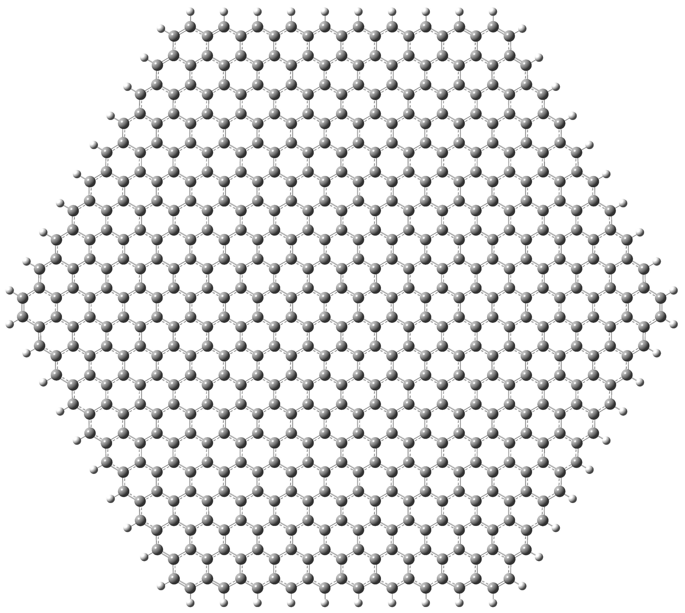
1. Introduction
2. Materials and Methods
3. Results and Discussion
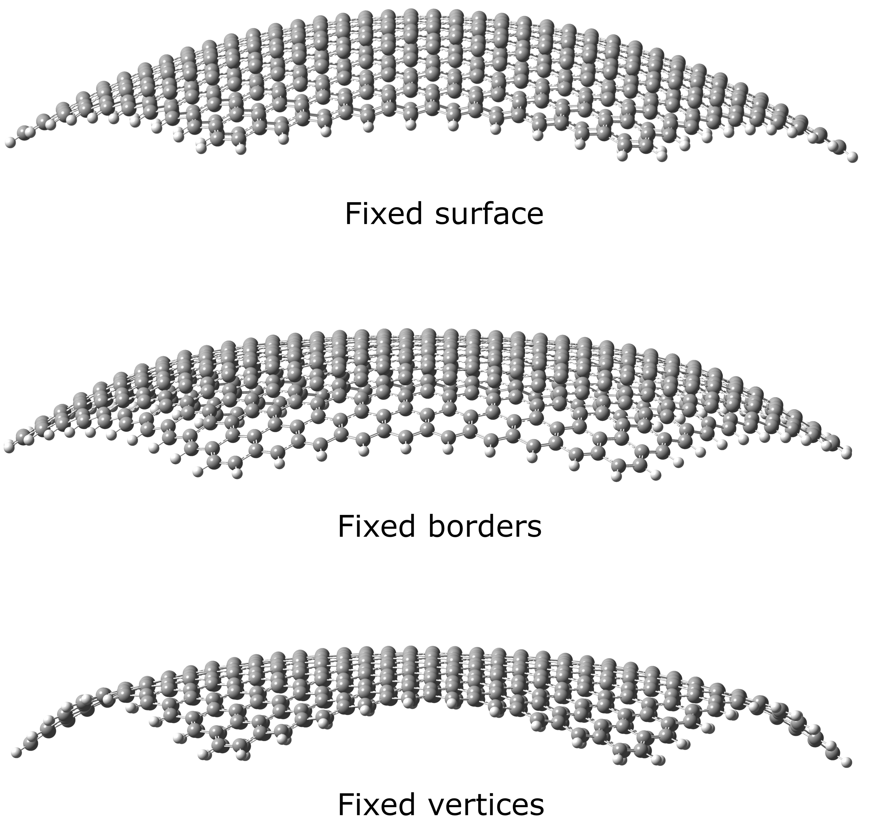
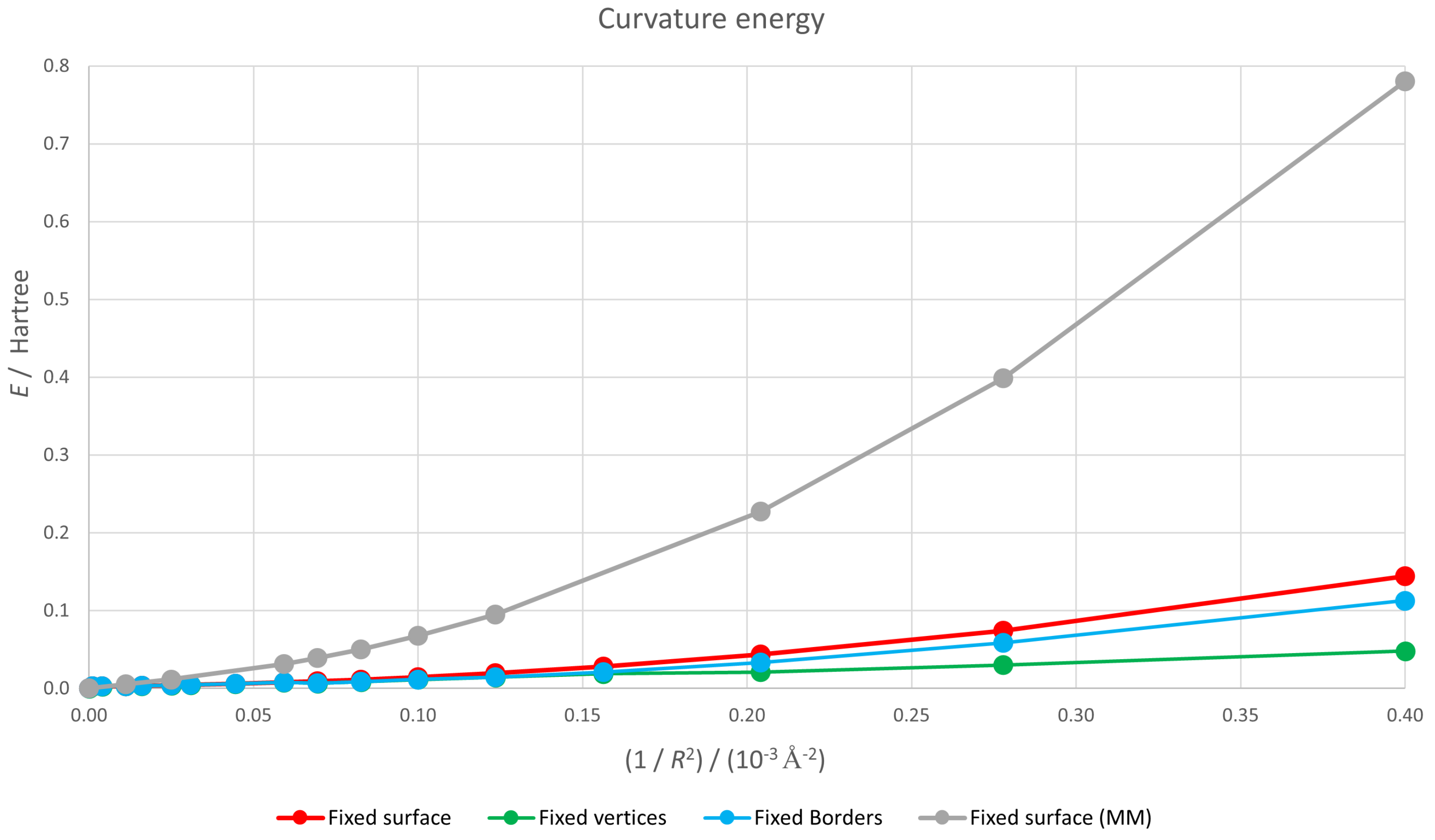
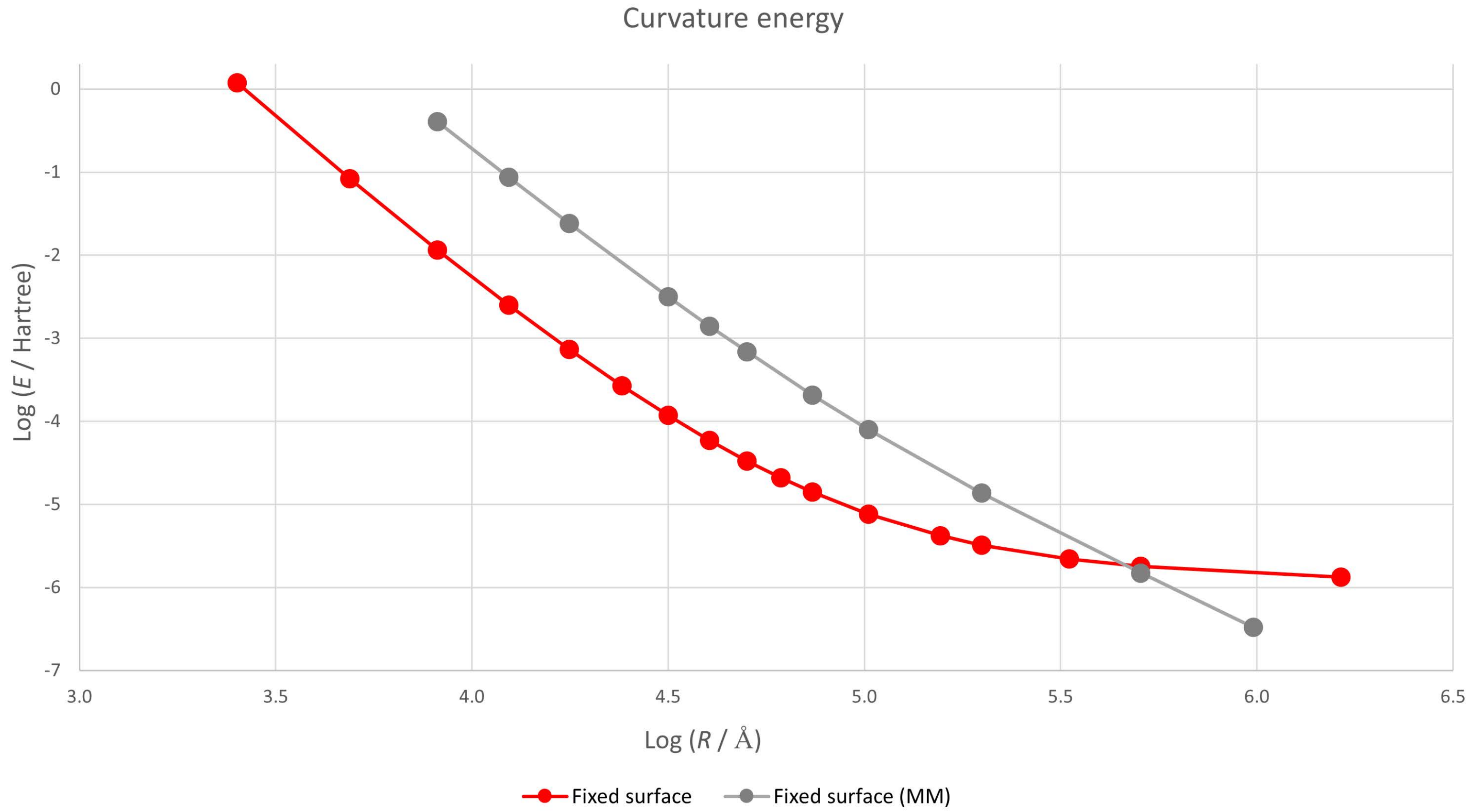
3.1. Curvature Energy
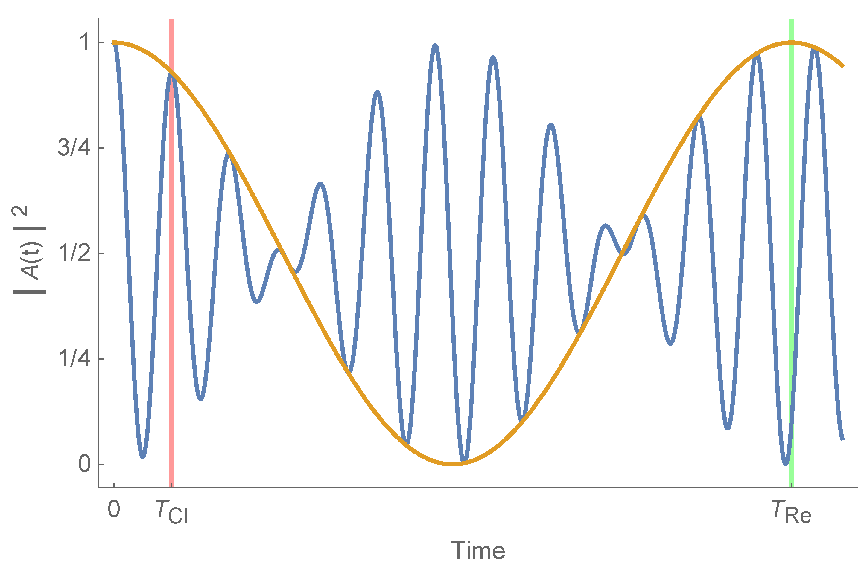
3.2. Quantum Revivals
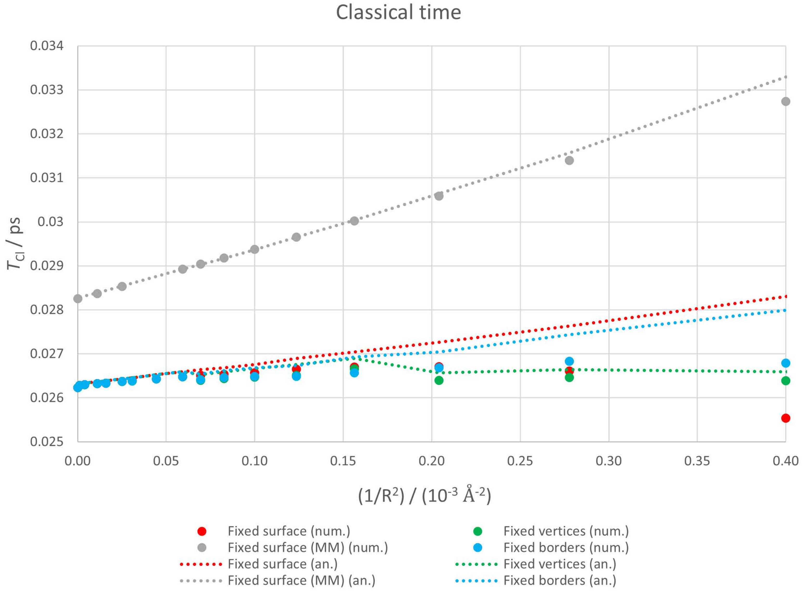
3.2.1. Classical Time
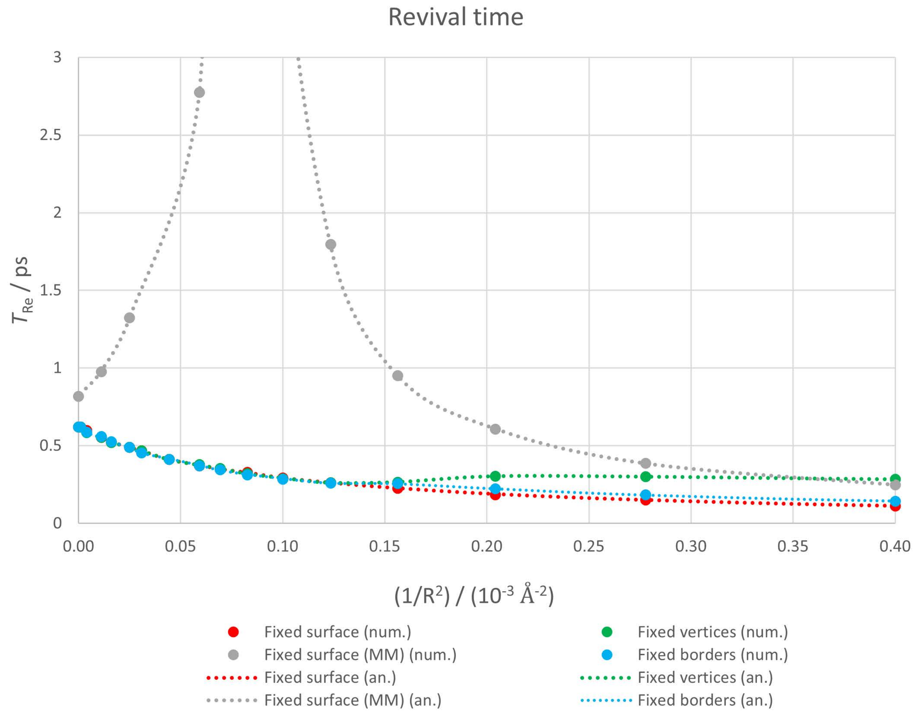
3.2.2. Revival Time
Author Contributions
Funding
Institutional Review Board Statement
Informed Consent Statement
Data Availability Statement
Conflicts of Interest
Abbreviations
| DFT | Density Functional Theory |
| GGA | Generalized Gradient Approximation |
| HF | Hartree-Fock |
| HOMO | Highest Occupied Molecular Orbital |
| LDA | Local Density Approximation |
| MM | Molecular Mechanics |
References
- Novoselov, K.S.; Geim, A.K.; Morozov, S.V.; Jiang, D.; Zhang, Y.; Dubonos, S.V.; Grigorieva, I.V.; Firsov, A.A. Electric Field Effect in Atomically Thin Carbon Films. Science 2004, 306, 666–669. [Google Scholar] [CrossRef]
- Web of Science™. Available online: https://www.webofscience.com (accessed on 22 April 2022).
- Lalwani, G.; Henslee, A.M.; Farshid, B.; Lin, L.; Kasper, F.K.; Qin, Y.X.; Mikos, A.G.; Sitharaman, B. Two-Dimensional Nanostructure-Reinforced Biodegradable Polymeric Nanocomposites for Bone Tissue Engineering. Biomacromolecules 2013, 14, 900–909. [Google Scholar] [CrossRef]
- Dimov, D.; Amit, I.; Gorrie, O.; Barnes, M.D.; Townsend, N.J.; Neves, A.I.S.; Withers, F.; Russo, S.; Craciun, M.F. Ultrahigh Performance Nanoengineered Graphene–Concrete Composites for Multifunctional Applications. Adv. Funct. Mater. 2018, 28, 1705183. [Google Scholar] [CrossRef]
- Berman, D.; Erdemir, A.; Sumant, A.V. Reduced wear and friction enabled by graphene layers on sliding steel surfaces in dry nitrogen. Carbon 2013, 59, 167–175. [Google Scholar] [CrossRef]
- Berman, D.; Deshmukh, S.A.; Sankaranarayanan, S.K.R.S.; Erdemir, A.; Sumant, A.V. Extraordinary Macroscale Wear Resistance of One Atom Thick Graphene Layer. Adv. Funct. Mater. 2014, 24, 6640–6646. [Google Scholar] [CrossRef]
- Li, X.; Chen, W.; Zhang, S.; Wu, Z.; Wang, P.; Xu, Z.; Chen, H.; Yin, W.; Zhong, H.; Lin, S. 18.5% efficient graphene/GaAs van der Waals heterostructure solar cell. Nano Energy 2015, 16, 310–319. [Google Scholar] [CrossRef]
- Stoller, M.D.; Park, S.; Zhu, Y.; An, J.; Ruoff, R.S. Graphene-Based Ultracapacitors. Nano Lett. 2008, 8, 3498–3502. [Google Scholar] [CrossRef] [PubMed]
- Zhao, J.; Zhang, J.; Yin, H.; Zhao, Y.; Xu, G.; Yuan, J.; Mo, X.; Tang, J.; Wang, F. Ultra-Fine Ruthenium Oxide Quantum Dots/Reduced Graphene Oxide Composite as Electrodes for High-Performance Supercapacitors. Nanomaterials 2022, 12, 1210. [Google Scholar] [CrossRef]
- Umar, M.; Nnadiekwe, C.C.; Haroon, M.; Abdulazeez, I.; Alhooshani, K.; Al-Saadi, A.A.; Peng, Q. A First-Principles Study on the Multilayer Graphene Nanosheets Anode Performance for Boron-Ion Battery. Nanomaterials 2022, 12, 1280. [Google Scholar] [CrossRef] [PubMed]
- Meng, S.; Wang, L.; Ji, X.; Yu, J.; Ma, X.; Zhang, J.; Zhao, W.; Ji, H.; Li, M.; Feng, H. Facile Gold-Nanoparticle Boosted Graphene Sensor Fabrication Enhanced Biochemical Signal Detection. Nanomaterials 2022, 12, 1327. [Google Scholar] [CrossRef]
- Askari, M.B.; Rozati, S.M.; Di Bartolomeo, A. Fabrication of Mn3O4-CeO2-rGO as Nanocatalyst for Electro-Oxidation of Methanol. Nanomaterials 2022, 12, 1187. [Google Scholar] [CrossRef] [PubMed]
- Oliveira, A.M.L.; Machado, M.; Silva, G.A.; Bitoque, D.B.; Tavares Ferreira, J.; Pinto, L.A.; Ferreira, Q. Graphene Oxide Thin Films with Drug Delivery Function. Nanomaterials 2022, 12, 1149. [Google Scholar] [CrossRef]
- Hu, S.; Lozada-Hidalgo, M.; Wang, F.; Mishchenko, A.; Schedin, F.; Nair, R.; Hill, E.; Boukhvalov, D.; Katsnelson, M.; Dryfe, R.; et al. Proton transport through one-atom-thick crystals. Nature 2014, 516, 227–230. [Google Scholar] [CrossRef] [PubMed]
- Wu, X.; Wang, D.; Kang, X.; Zhang, D.; Yan, Y.; Guo, G.; Sun, Z.; Wang, X. Displacement Reaction-Assisted Synthesis of Sub-Nanometer Pt/Bi Boost Methanol-Tolerant Fuel Cells. Nanomaterials 2022, 12, 1301. [Google Scholar] [CrossRef] [PubMed]
- Mangum, J.M.; Harerimana, F.; Gikunda, M.N.; Thibado, P.M. Mechanisms of Spontaneous Curvature Inversion in Compressed Graphene Ripples for Energy Harvesting Applications via Molecular Dynamics Simulations. Membranes 2021, 11, 516. [Google Scholar] [CrossRef] [PubMed]
- Robinett, R. Quantum wave packet revivals. Phys. Rep. 2004, 392, 1–119. [Google Scholar] [CrossRef]
- Dooley, S.; Spiller, T.P. Fractional revivals, multiple-Schrödinger-cat states, and quantum carpets in the interaction of a qubit with N qubits. Phys. Rev. A 2014, 90, 012320. [Google Scholar] [CrossRef]
- Li, K.; Xia, F.; Wang, M.; Sun, P.; Liu, T.; Hu, W.; Kong, W.; Yun, M.; Dong, L. Discrete Talbot effect in dielectric graphene plasmonic waveguide arrays. Carbon 2017, 118, 192–199. [Google Scholar] [CrossRef]
- Kolaric, B.; Maes, B.; Clays, K.; Durt, T.; Caudano, Y. Strong Light–Matter Coupling as a New Tool for Molecular and Material Engineering: Quantum Approach. Adv. Quantum Technol. 2018, 1, 1800001. [Google Scholar] [CrossRef]
- Tsarev, M.V.; Ryabov, A.; Baum, P. Free-electron qubits and maximum-contrast attosecond pulses via temporal Talbot revivals. Phys. Rev. Res. 2021, 3, 043033. [Google Scholar] [CrossRef]
- Krueckl, V.; Kramer, T. Revivals of quantum wave packets in graphene. New J. Phys. 2009, 11, 093010. [Google Scholar] [CrossRef]
- Ali, R.; Saif, F. Chiral phase transition and quantum revivals in graphene. Mater. Res. Express 2015, 2, 095602. [Google Scholar] [CrossRef]
- Díaz-Bautista, E.; Betancur-Ocampo, Y. Phase-space representation of Landau and electron coherent states for uniaxially strained graphene. Phys. Rev. B 2020, 101, 125402. [Google Scholar] [CrossRef]
- López, A.; Di Teodoro, A.; Schliemann, J.; Berche, B.; Santos, B. Laser-induced modulation of the Landau level structure in single-layer graphene. Phys. Rev. B 2015, 92, 235411. [Google Scholar] [CrossRef]
- García, T.; Rodríguez-Bolívar, S.; Cordero, N.A.; Romera, E. Wavepacket revivals in monolayer and bilayer graphene rings. J. Phy. Condens. Matter 2013, 25, 235301. [Google Scholar] [CrossRef]
- García, T.; Cordero, N.A.; Romera, E. Zitterbewegung and quantum revivals in monolayer graphene quantum dots in magnetic fields. Phys. Rev. B 2014, 89, 075416. [Google Scholar] [CrossRef]
- Peierls, R. Quelques propriétés typiques des corps solides. Ann. L’inst. Henri Poincare 1935, 5, 177–222. [Google Scholar]
- Landau, L.D. On the theory of phase transitions. Zh. Eksp. Teor. Fiz. 1937, 7, 19–32, English Translation in Ukr. J. Phys. 2008, 53, 25–35. [Google Scholar] [CrossRef]
- Meyer, J.; Geim, A.; Katsnelson, M.; Novoselov, K.; Obergfell, D.; Roth, S.; Girit, C.; Zettl, A. On the roughness of single- and bi-layer graphene membranes. Solid State Commun. 2007, 143, 101–109. [Google Scholar] [CrossRef]
- Meyer, J.C.; Geim, A.K.; Katsnelson, M.I.; Novoselov, K.S.; Booth, T.J.; Roth, S. The structure of suspended graphene sheets. Nature 2007, 446, 60–63. [Google Scholar] [CrossRef] [PubMed]
- Deng, S.; Berry, V. Wrinkled, rippled and crumpled graphene: An overview of formation mechanism, electronic properties, and applications. Mater. Today 2016, 19, 197–212. [Google Scholar] [CrossRef]
- Fasolino, A.; Los, J.; Katsnelson, M. Intrinsic ripples in graphene. Nat. Mater. 2007, 6, 858–861. [Google Scholar] [CrossRef]
- Carlsson, J. Buckle or break. Nat. Mater. 2007, 6, 801–802. [Google Scholar] [CrossRef] [PubMed][Green Version]
- Lundeberg, M.B.; Folk, J.A. Rippled Graphene in an In-Plane Magnetic Field: Effects of a Random Vector Potential. Phys. Rev. Lett. 2010, 105, 146804. [Google Scholar] [CrossRef]
- Los, J.H.; Ghiringhelli, L.M.; Meijer, E.J.; Fasolino, A. Improved long-range reactive bond-order potential for carbon. I. Construction. Phys. Rev. B 2005, 72, 214102. [Google Scholar] [CrossRef]
- Ishigami, M.; Chen, J.H.; Cullen, W.G.; Fuhrer, M.S.; Williams, E.D. Atomic Structure of Graphene on SiO2. Nano Lett. 2007, 7, 1643–1648. [Google Scholar] [CrossRef]
- Geringer, V.; Liebmann, M.; Echtermeyer, T.; Runte, S.; Schmidt, M.; Rückamp, R.; Lemme, M.C.; Morgenstern, M. Intrinsic and extrinsic corrugation of monolayer graphene deposited on SiO2. Phys. Rev. Lett. 2009, 102, 076102. [Google Scholar] [CrossRef] [PubMed]
- Stolyarova, E.; Stolyarov, D.; Bolotin, K.; Ryu, S.; Liu, L.; Rim, K.T.; Klima, M.; Hybertsen, M.; Pogorelsky, I.; Pavlishin, I.; et al. Observation of Graphene Bubbles and Effective Mass Transport under Graphene Films. Nano Lett. 2009, 9, 332–337. [Google Scholar] [CrossRef]
- Leconte, N.; Kim, H.; Kim, H.J.; Ha, D.H.; Watanabe, K.; Taniguchi, T.; Jung, J.; Jung, S. Graphene bubbles and their role in graphene quantum transport. Nanoscale 2017, 9, 6041–6047. [Google Scholar] [CrossRef]
- Georgiou, T.; Britnell, L.; Blake, P.; Gorbachev, R.V.; Gholinia, A.; Geim, A.K.; Casiraghi, C.; Novoselov, K.S. Graphene bubbles with controllable curvature. Appl. Phys. Lett. 2011, 99, 093103. [Google Scholar] [CrossRef]
- Huamán, A.; Foa Torres, L.E.F.; Balseiro, C.A.; Usaj, G. Quantum Hall edge states under periodic driving: A Floquet induced chirality switch. Phys. Rev. Res. 2021, 3, 013201. [Google Scholar] [CrossRef]
- Ornigotti, M.; Ornigotti, L.; Biancalana, F. Generation of half-integer harmonics and efficient THz-to-visible frequency conversion in strained graphene. APL Photon. 2021, 6, 060801. [Google Scholar] [CrossRef]
- Sinha, D.; Berche, B. Quantum oscillations and wave packet revival in conical graphene. Eur. Phys. J. B 2016, 89, 57. [Google Scholar] [CrossRef][Green Version]
- Belouad, A.; Jellal, A.; Bahlouli, H. Electronic properties of graphene quantum ring with wedge disclination. Eur. Phys. J. B 2021, 94, 1–10. [Google Scholar] [CrossRef]
- Wallace, P.R. The Band Theory of Graphite. Phys. Rev. 1947, 71, 622–634. [Google Scholar] [CrossRef]
- Hohenberg, P.; Kohn, W. Inhomogeneous Electron Gas. Phys. Rev. 1964, 136, B864–B871. [Google Scholar] [CrossRef]
- Kohn, W.; Sham, L.J. Self-Consistent Equations Including Exchange and Correlation Effects. Phys. Rev. 1965, 140, A1133–A1138. [Google Scholar] [CrossRef]
- Vosko, S.H.; Wilk, L.; Nusair, M. Accurate spin-dependent electron liquid correlation energies for local spin density calculations: A critical analysis. Can. J. Phys. 1980, 58, 1200–1211. [Google Scholar] [CrossRef]
- Frisch, M.J.; Trucks, G.W.; Schlegel, H.B.; Scuseria, G.E.; Robb, M.A.; Cheeseman, J.R.; Scalmani, G.; Barone, V.; Mennucci, B.; Petersson, G.A.; et al. Gaussian 09, 2009; Gaussian Inc.: Wallingford, CT, USA, 2009. [Google Scholar]
- Frisch, M.J.; Trucks, G.W.; Schlegel, H.B.; Scuseria, G.E.; Robb, M.A.; Cheeseman, J.R.; Scalmani, G.; Barone, V.; Petersson, G.A.; Nakatsuji, H.; et al. Gaussian 16, 2016; Gaussian Inc.: Wallingford, CT, USA, 2016. [Google Scholar]
- Girifalco, L.A.; Hodak, M. Van der Waals binding energies in graphitic structures. Phys. Rev. B 2002, 65, 125404. [Google Scholar] [CrossRef]
- Hasegawa, M.; Nishidate, K. Semiempirical approach to the energetics of interlayer binding in graphite. Phys. Rev. B 2004, 70, 205431. [Google Scholar] [CrossRef]
- Torres-Rojas, R.M.; Contreras-Solorio, D.A.; Hernández, L.; Enciso, A. Band gap variation in bi, tri and few-layered 2D graphene/hBN heterostructures. Solid State Commun. 2022, 341, 114553. [Google Scholar] [CrossRef]
- Khantha, M.; Cordero, N.A.; Molina, L.M.; Alonso, J.A.; Girifalco, L.A. Interaction of lithium with graphene: An ab initio study. Phys. Rev. B 2004, 70, 125422. [Google Scholar] [CrossRef]
- Cordero, N.A.; Alonso, J.A. The interaction of sulfuric acid with graphene and formation of adsorbed crystals. Nanotechnology 2007, 18, 485705. [Google Scholar] [CrossRef]
- Khantha, M.; Cordero, N.A.; Alonso, J.A.; Cawkwell, M.; Girifalco, L.A. Interaction and concerted diffusion of lithium in a (5,5) carbon nanotube. Phys. Rev. B 2008, 78, 115430. [Google Scholar] [CrossRef]
- Cordero, N.A.; Alonso, J.A. Interaction of Surfactants Containing a Sulfuric Group with a (5,5) Carbon Nanotube. J. Phys. Chem. C 2010, 114, 17249–17256. [Google Scholar] [CrossRef]
- Ayala, I.G.; Cordero, N.A.; Alonso, J.A. Surfactant effect of sulfuric acid on the exfoliation of bilayer graphene. Phys. Rev. B 2011, 84, 165424. [Google Scholar] [CrossRef]
- Ayala, I.G.; Cordero, N.A. Interaction of sodium bisulfate with mono- and bi-layer graphene. J. Nanopart. Res. 2012, 14, 1071. [Google Scholar] [CrossRef]
- Zhao, F.; Cao, T.; Louie, S.G. Topological Phases in Graphene Nanoribbons Tuned by Electric Fields. Phys. Rev. Lett. 2021, 127, 166401. [Google Scholar] [CrossRef]
- Ditchfield, R.; Hehre, W.J.; Pople, J.A. Self-Consistent Molecular-Orbital Methods. IX. An Extended Gaussian-Type Basis for Molecular-Orbital Studies of Organic Molecules. J. Chem. Phys. 1971, 54, 724–728. [Google Scholar] [CrossRef]
- Hehre, W.J.; Ditchfield, R.; Pople, J.A. Self—Consistent Molecular Orbital Methods. XII. Further Extensions of Gaussian—Type Basis Sets for Use in Molecular Orbital Studies of Organic Molecules. J. Chem. Phys. 1972, 56, 2257–2261. [Google Scholar] [CrossRef]
- Hariharan, P.; Pople, J.A. The influence of polarization functions on molecular orbital hydrogenation energies. Theor. Chim. Acta 1973, 28, 213–222. [Google Scholar] [CrossRef]
- Hariharan, P.; Pople, J. Accuracy of AHn equilibrium geometries by single determinant molecular orbital theory. Mol. Phys. 1974, 27, 209–214. [Google Scholar] [CrossRef]
- Gordon, M.S. The isomers of silacyclopropane. Chem. Phys. Lett. 1980, 76, 163–168. [Google Scholar] [CrossRef]
- Francl, M.M.; Pietro, W.J.; Hehre, W.J.; Binkley, J.S.; Gordon, M.S.; DeFrees, D.J.; Pople, J.A. Self-consistent molecular orbital methods. XXIII. A polarization-type basis set for second-row elements. J. Chem. Phys. 1982, 77, 3654–3665. [Google Scholar] [CrossRef]
- Sun, Q.; Yao, X.; Gröning, O.; Eimre, K.; Pignedoli, C.A.; Müllen, K.; Narita, A.; Fasel, R.; Ruffieux, P. Coupled Spin States in Armchair Graphene Nanoribbons with Asymmetric Zigzag Edge Extensions. Nano Lett. 2020, 20, 6429–6436. [Google Scholar] [CrossRef]
- Dennington, R.; Keith, T.A.; Millam, J.M. GaussView Version 6, 2019; Semichem Inc.: Shawnee Mission, KS, USA, 2019. [Google Scholar]
- Zhou, Y.; Chen, Y.; Liu, B.; Wang, S.; Yang, Z.; Hu, M. Mechanics of nanoscale wrinkling of graphene on a non-developable surface. Carbon 2015, 84, 263–271. [Google Scholar] [CrossRef]
- Alber, G.; Ritsch, H.; Zoller, P. Generation and detection of Rydberg wave packets by short laser pulses. Phys. Rev. A 1986, 34, 1058–1064. [Google Scholar] [CrossRef]
- Yeazell, J.A.; Mallalieu, M.; Stroud, C.R. Observation of the collapse and revival of a Rydberg electronic wave packet. Phys. Rev. Lett. 1990, 64, 2007–2010. [Google Scholar] [CrossRef]
- Wals, J.; Fielding, H.H.; Christian, J.F.; Snoek, L.C.; van der Zande, W.J.; van Linden van den Heuvell, H.B. Observation of Rydberg wave packet dynamics in a Coulombic and magnetic field. Phys. Rev. Lett. 1994, 72, 3783–3786. [Google Scholar] [CrossRef]
- Dantus, M.; Rosker, M.J.; Zewail, A.H. Real-time femtosecond probing of “transition states” in chemical reactions. J. Chem. Phys. 1987, 87, 2395–2397. [Google Scholar] [CrossRef]
- Bowman, R.; Dantus, M.; Zewail, A. Femtosecond transition-state spectroscopy of iodine: From strongly bound to repulsive surface dynamics. Chem. Phys. Lett. 1989, 161, 297–302. [Google Scholar] [CrossRef]
- Dong, S.; Trivedi, D.; Chakrabortty, S.; Kobayashi, T.; Chan, Y.; Prezhdo, O.V.; Loh, Z.H. Observation of an Excitonic Quantum Coherence in CdSe Nanocrystals. Nano Lett. 2015, 15, 6875–6882. [Google Scholar] [CrossRef] [PubMed]
- Scilab. Available online: https://www.scilab.org/ (accessed on 22 April 2022).
- Mathematica. 2021. Available online: https://www.wolfram.com/mathematica (accessed on 22 April 2022).
- Bolívar, J.C.; Cordero, N.A.; Nagy, A.; Romera, E. Fidelity as a marker of topological phase transitions in 2D Dirac materials. Int. J. Quantum Chem. 2018, 118, e25674. [Google Scholar] [CrossRef]


Publisher’s Note: MDPI stays neutral with regard to jurisdictional claims in published maps and institutional affiliations. |
© 2022 by the authors. Licensee MDPI, Basel, Switzerland. This article is an open access article distributed under the terms and conditions of the Creative Commons Attribution (CC BY) license (https://creativecommons.org/licenses/by/4.0/).
Share and Cite
de-la-Huerta-Sainz, S.; Ballesteros, A.; Cordero, N.A. Quantum Revivals in Curved Graphene Nanoflakes. Nanomaterials 2022, 12, 1953. https://doi.org/10.3390/nano12121953
de-la-Huerta-Sainz S, Ballesteros A, Cordero NA. Quantum Revivals in Curved Graphene Nanoflakes. Nanomaterials. 2022; 12(12):1953. https://doi.org/10.3390/nano12121953
Chicago/Turabian Stylede-la-Huerta-Sainz, Sergio, Angel Ballesteros, and Nicolás A. Cordero. 2022. "Quantum Revivals in Curved Graphene Nanoflakes" Nanomaterials 12, no. 12: 1953. https://doi.org/10.3390/nano12121953
APA Stylede-la-Huerta-Sainz, S., Ballesteros, A., & Cordero, N. A. (2022). Quantum Revivals in Curved Graphene Nanoflakes. Nanomaterials, 12(12), 1953. https://doi.org/10.3390/nano12121953