Kirkwood-Buff Integrals Using Molecular Simulation: Estimation of Surface Effects

 , , , ,
Abstract
:1. Introduction
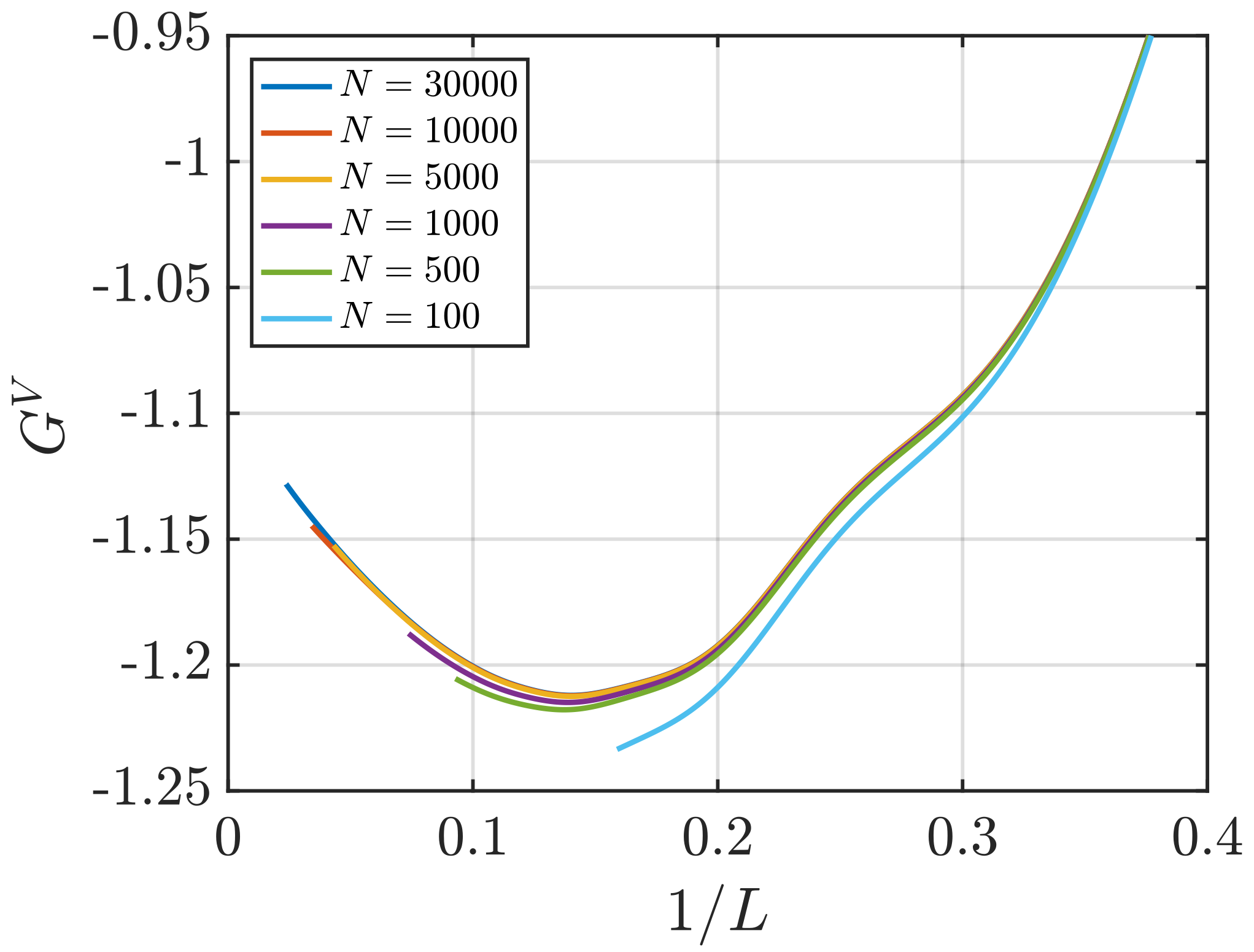
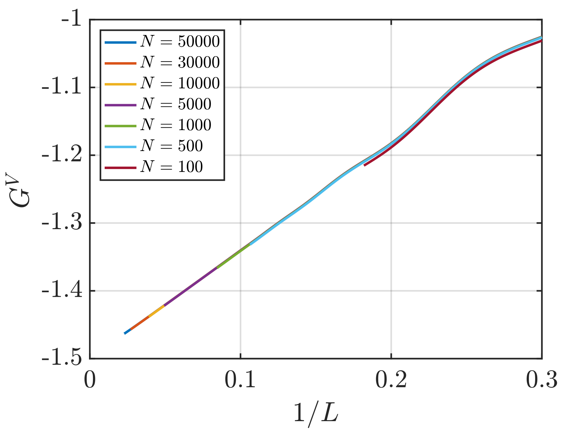
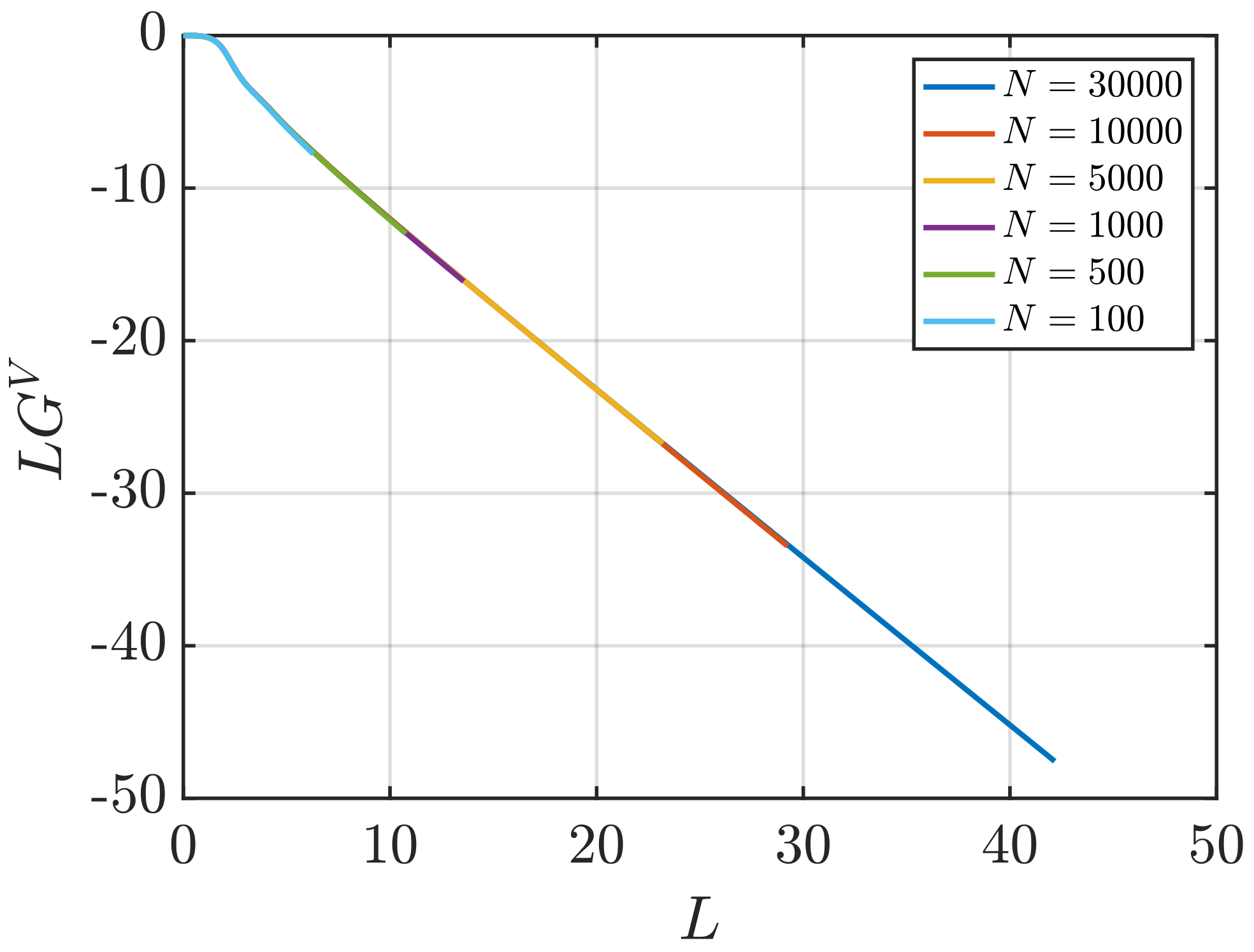
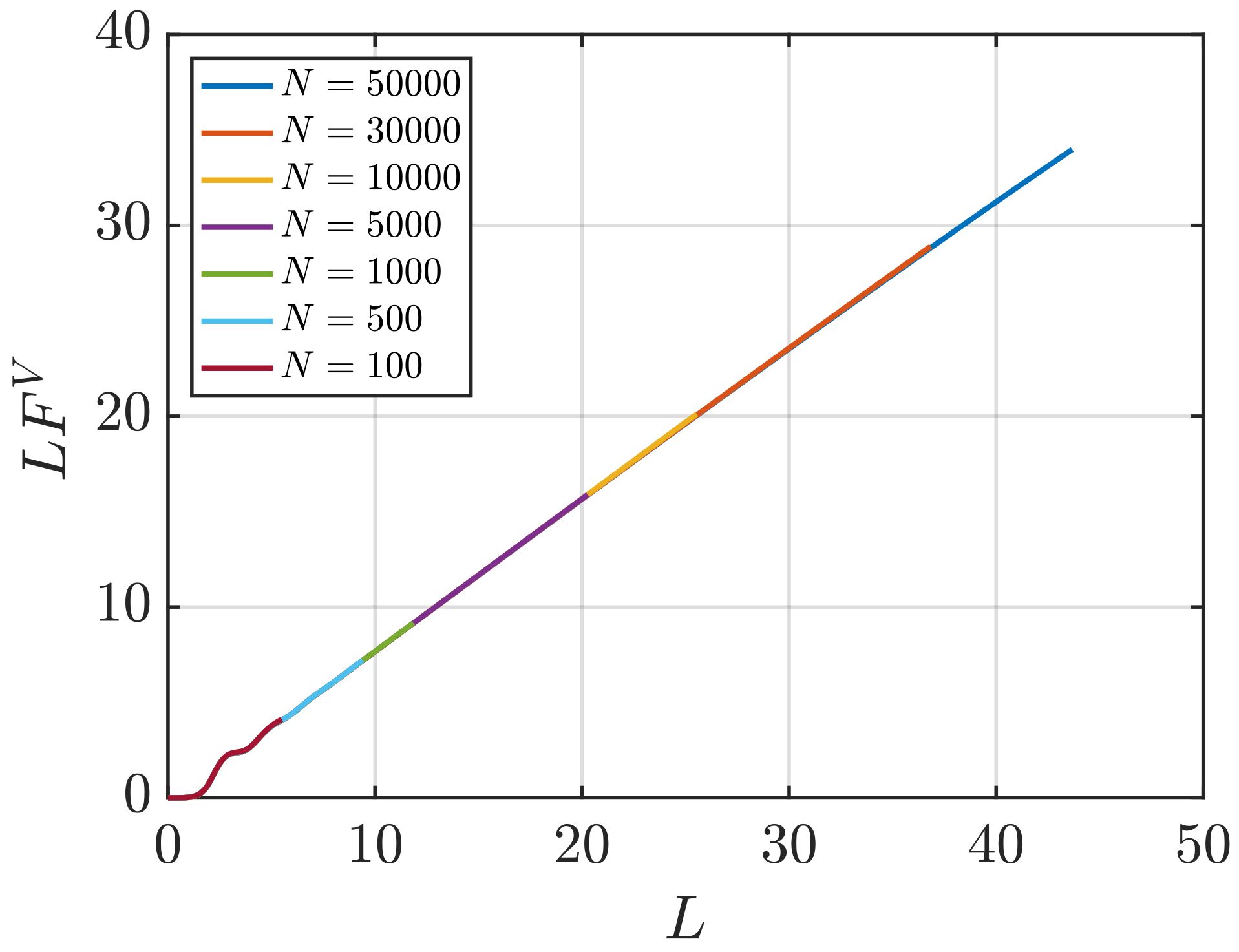
- Using the scaling of (Equation (4)) with . To estimate , the linear regime of the scaling is extrapolated to the limit .
2. Methods
Simulation Details
3. Results
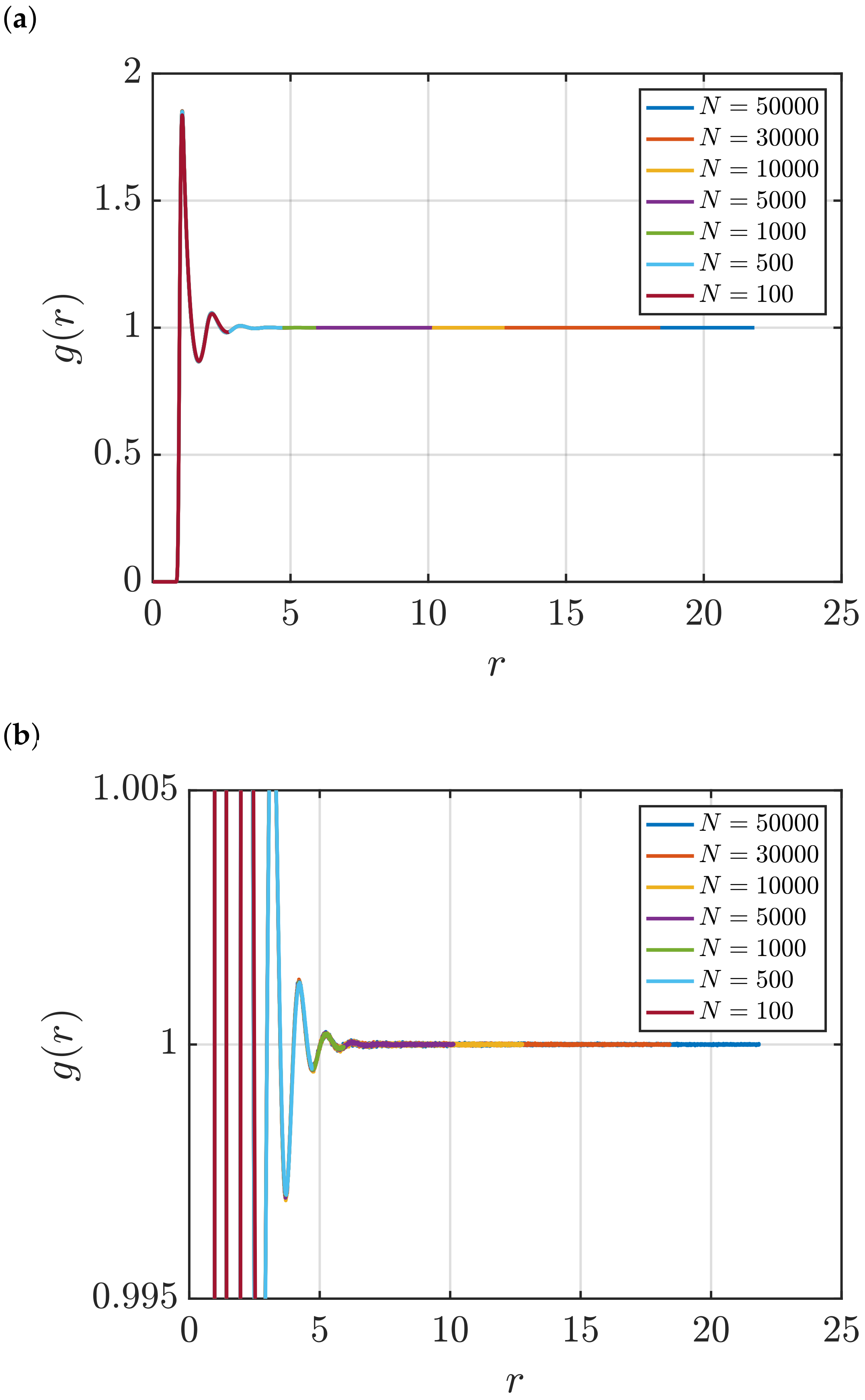
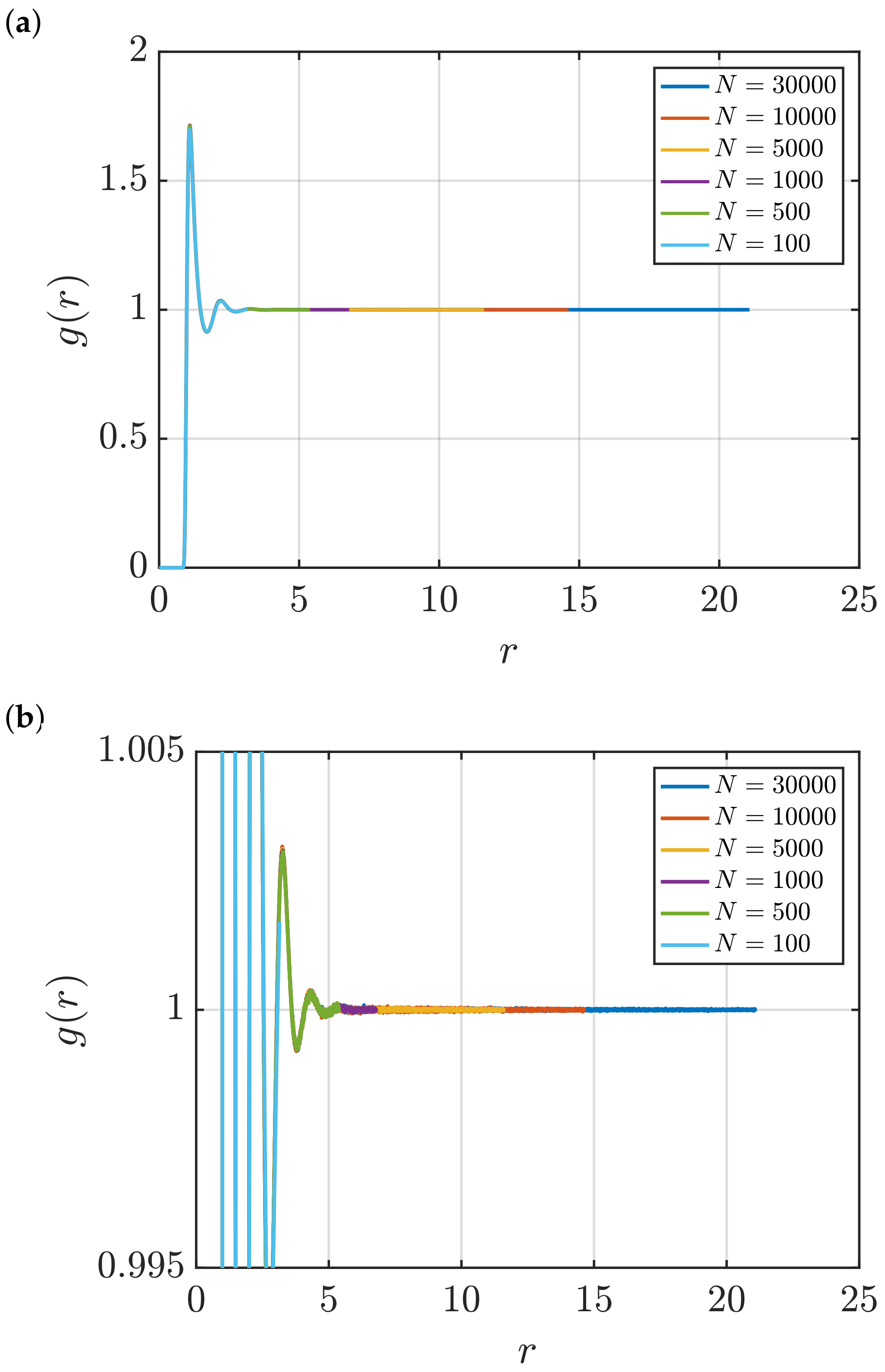
3.1. Estimation of KB Integrals
Effect of System Size and Density
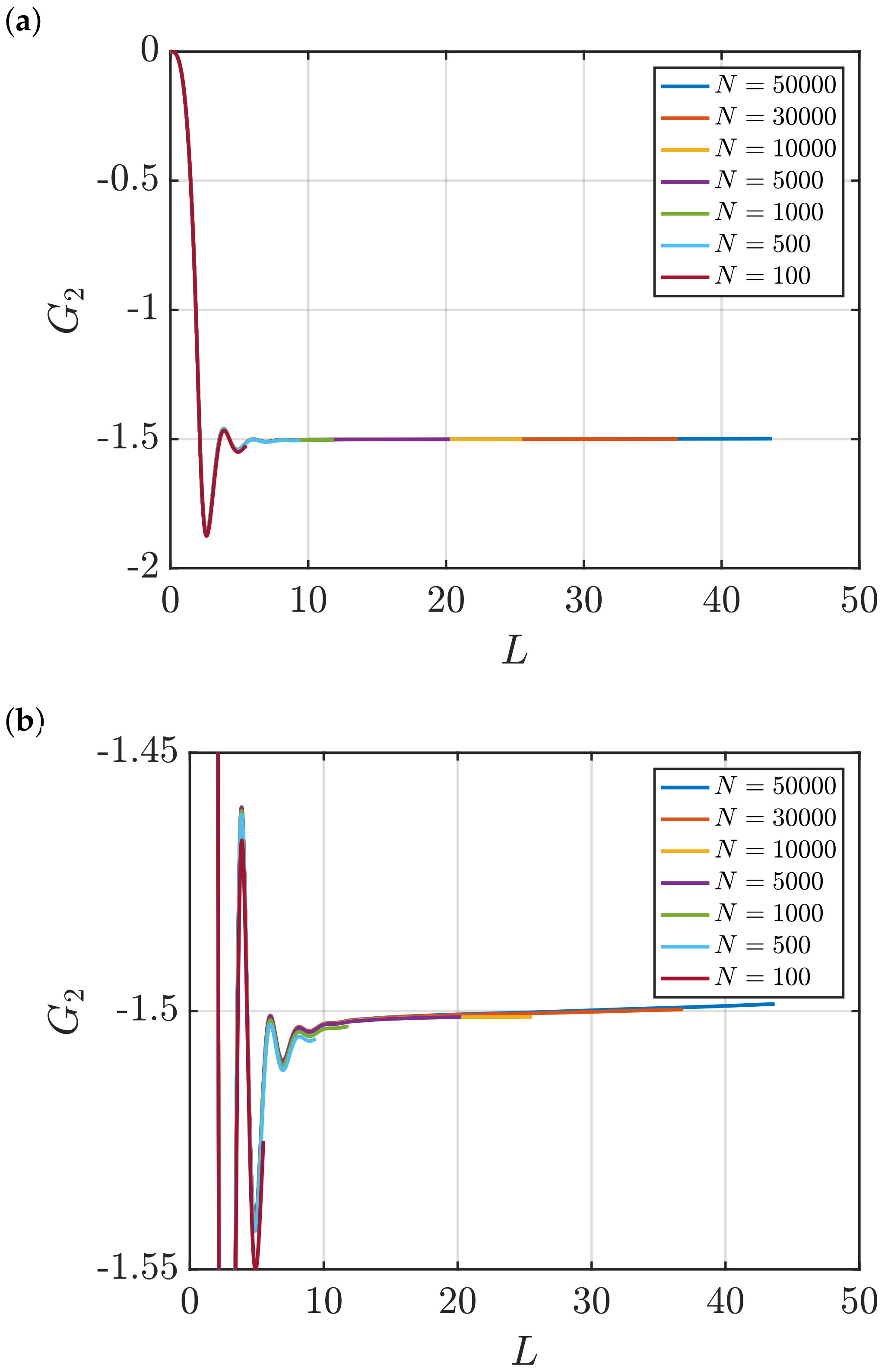
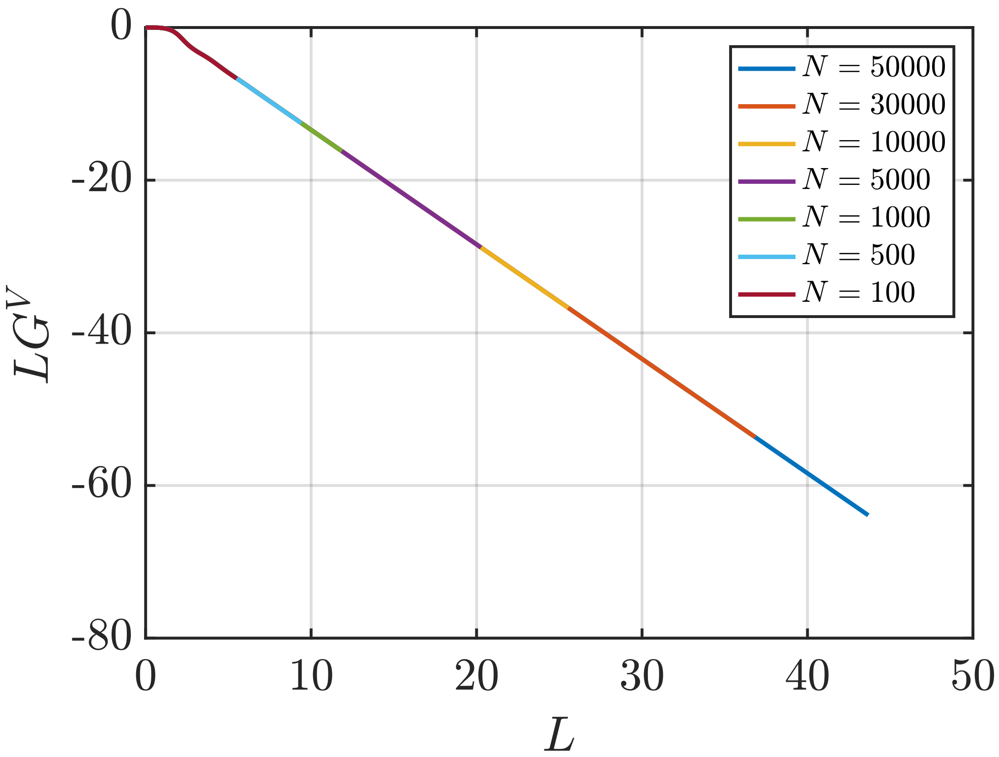
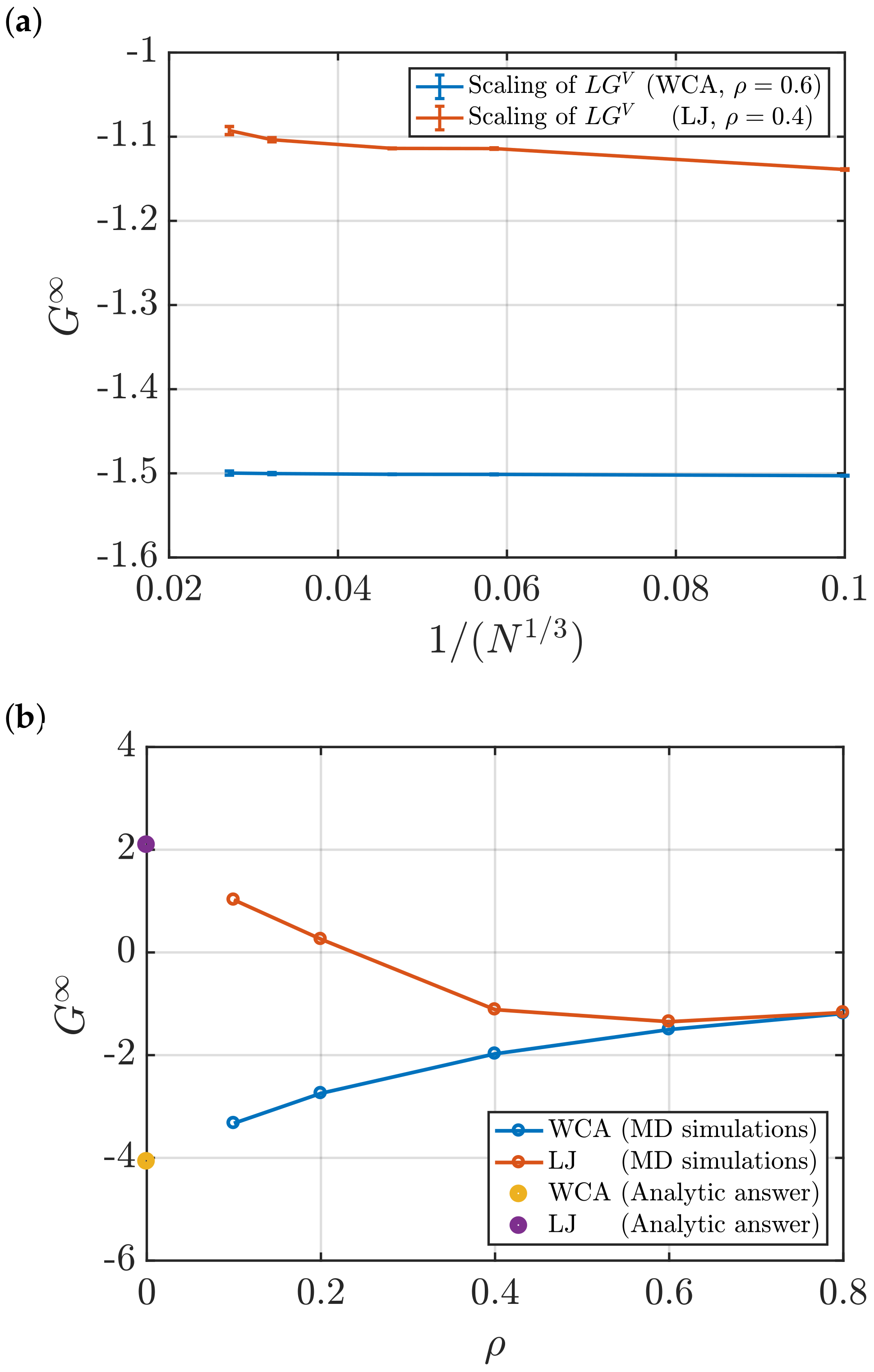
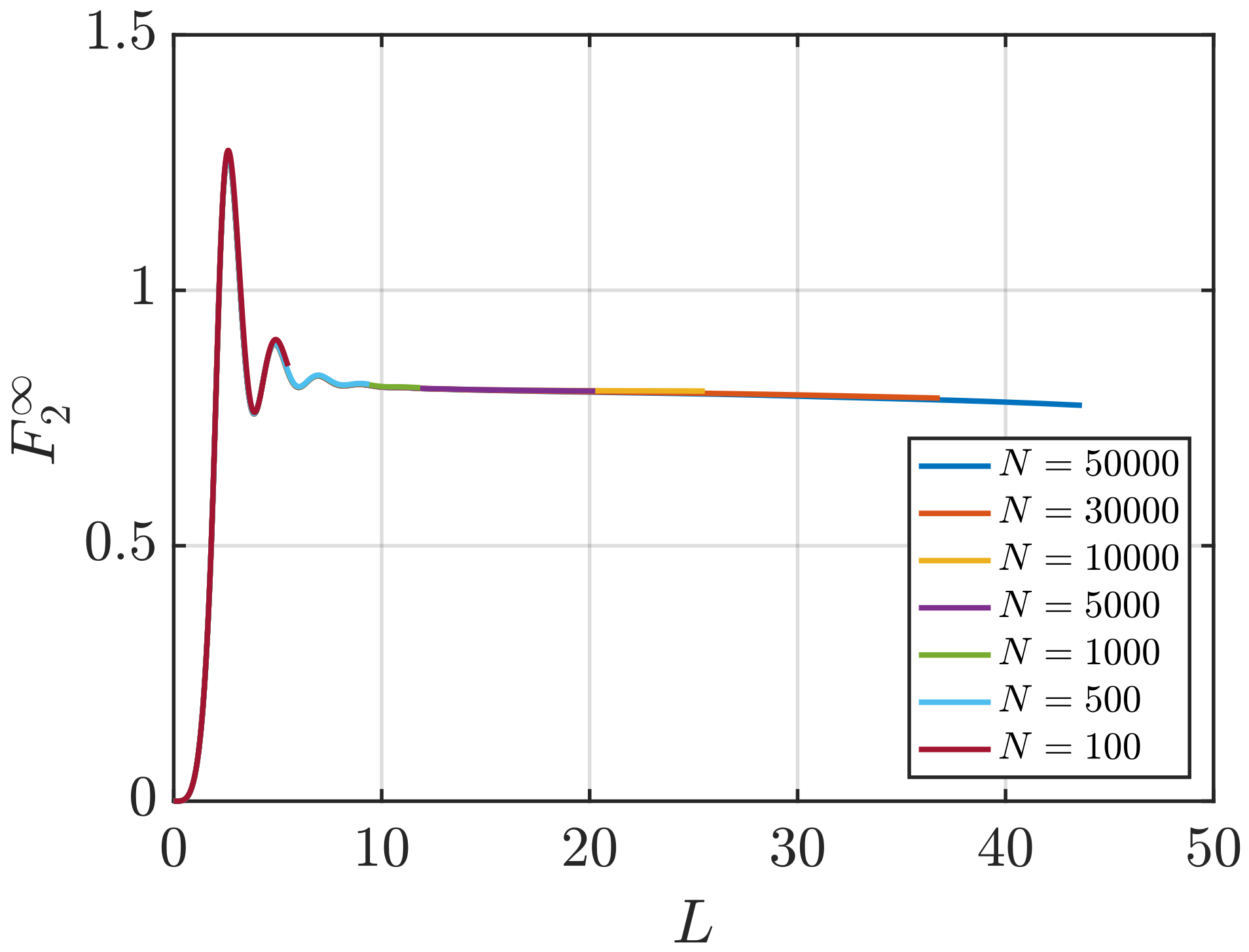
3.2. Estimation of Surface Effects
Effect of System Size and Density
4. Conclusions
Supplementary Materials
Author Contributions
Funding
Conflicts of Interest
References
- Patterson, D. Effects of molecular size and shape in solution thermodynamics. Pure Appl. Chem. 1976, 47, 305–314. [Google Scholar] [CrossRef]
- Koga, Y. Solution Thermodynamics and Its Application to Aqueous Solutions: A Differential Approach, 2nd ed.; Elsevier: Amsterdam, The Netherlands, 2017. [Google Scholar]
- Lee, L.L. Molecular Thermodynamics of Non-Ideal Fluids; Butterworth-Heinemann: Oxford, UK, 2016. [Google Scholar]
- Panagiotopoulos, A.Z. Molecular simulation of phase equilibria: Simple, ionic and polymeric fluids. Fluid Phase Equilib. 1992, 76, 97–112. [Google Scholar] [CrossRef]
- Schnell, S.K.; Skorpa, R.; Bedeaux, D.; Kjelstrup, S.; Vlugt, T.J.H.; Simon, J.M. Partial molar enthalpies and reaction enthalpies from equilibrium molecular dynamics simulation. J. Chem. Phys. 2014, 141, 144501. [Google Scholar] [CrossRef] [Green Version]
- Kirkwood, J.G.; Buff, F.P. The Statistical Mechanical Theory of Solutions. I. J. Chem. Phys. 1951, 19, 774–777. [Google Scholar] [CrossRef]
- Ben-Naim, A. Molecular Theory of Solutions; Oxford University Press: Oxford, UK, 2006. [Google Scholar]
- Hall, D.G. Kirkwood–Buff theory of solutions. An alternative derivation of part of it and some applications. Trans. Faraday Soc. 1971, 67, 2516–2524. [Google Scholar] [CrossRef]
- Newman, K.E. Kirkwood–Buff solution theory: Derivation and applications. Chem. Soc. Rev. 1994, 23, 31–40. [Google Scholar] [CrossRef]
- Dawass, N.; Krüger, P.; Schnell, S.K.; Simon, J.M.; Vlugt, T.J.H. Kirkwood-Buff integrals from molecular simulation. Fluid Phase Equilib. 2019, 486, 21–36. [Google Scholar] [CrossRef]
- Schnell, S.K.; Liu, X.; Simon, J.M.; Bardow, A.; Bedeaux, D.; Vlugt, T.J.H.; Kjelstrup, S. Calculating thermodynamic properties from fluctuations at small scales. J. Phys. Chem. B 2011, 115, 10911–10918. [Google Scholar] [CrossRef]
- Krüger, P.; Schnell, S.K.; Bedeaux, D.; Kjelstrup, S.; Vlugt, T.J.H.; Simon, J.M. Kirkwood–Buff Integrals for Finite Volumes. J. Phys. Chem. Lett. 2013, 4, 235–238. [Google Scholar] [CrossRef]
- Hill, T.L. Thermodynamics of Small Systems. J. Chem. Phys. 1962, 36, 3182–3197. [Google Scholar] [CrossRef]
- Hill, T.L. Thermodynamics of Small Systems; Dover: New York, NY, USA, 1994. [Google Scholar]
- Dawass, N.; Krüger, P.; Schnell, S.K.; Bedeaux, D.; Kjelstrup, S.; Simon, J.M.; Vlugt, T.J.H. Finite-size effects of Kirkwood–Buff integrals from molecular simulations. Mol. Simu. 2018, 44, 599–612. [Google Scholar] [CrossRef]
- Krüger, P.; Vlugt, T.J.H. Size and shape dependence of finite–volume Kirkwood-Buff integrals. Phys. Rev. E 2018, 97, 051301. [Google Scholar] [CrossRef] [PubMed] [Green Version]
- Strøm, B.A.; Simon, J.M.; Schnell, S.K.; Kjelstrup, S.; He, J.; Bedeaux, D. Size and shape effects on the thermodynamic properties of nanoscale volumes of water. Phys. Chem. Chem. Phys. 2017, 19, 9016–9027. [Google Scholar] [CrossRef] [PubMed]
- Frenkel, D.; Smit, B. Understanding Molecular Simulation: From Algorithms to Applications, 2nd ed.; Academic Press: London, UK, 2002; Volume 1. [Google Scholar]
- Dawass, N.; Krüger, P.; Schnell, S.K.; Simon, J.M.; Vlugt, T.J.H. Kirkwood–Buff integrals of finite systems: Shape effects. Mol. Phys. 2018, 116, 1573–1580. [Google Scholar] [CrossRef] [Green Version]
- Santos, A. Finite-size estimates of Kirkwood-Buff and similar integrals. Phys. Rev. E 2018, 98, 063302. [Google Scholar] [CrossRef] [Green Version]
- Lennard-Jones, J.E. On the determination of molecular fields. II. From the equation of state of gas. Proc. R. Soc. A 1924, 106, 463–477. [Google Scholar]
- Weeks, J.D.; Chandler, D.; Andersen, H.C. Role of Repulsive Forces in Determining the Equilibrium Structure of Simple Liquids. J. Chem. Phys. 1971, 54, 5237–5247. [Google Scholar] [CrossRef]
- Borgis, D.; Assaraf, R.; Rotenberg, B.; Vuilleumier, R. Computation of pair distribution functions and three-dimensional densities with a reduced variance principle. Mol. Phys. 2013, 111, 3486–3492. [Google Scholar] [CrossRef]
- De las Heras, D.; Schmidt, M. Better than counting: Density profiles from force sampling. Phys. Rev. Lett. 2018, 120, 218001. [Google Scholar] [CrossRef] [Green Version]
- Jamali, S. Transport Properties of Fluids: Methodology and Force Field Improvement Using Molecular Dynamics Simulations. Ph.D. Thesis, Delft University of Technology, Delft, The Netherlands, 2020. [Google Scholar]
- Ganguly, P.; van der Vegt, N.F.A. Convergence of Sampling Kirkwood-Buff Integrals of Aqueous Solutions with Molecular Dynamics Simulations. J. Chem. Theory Comput. 2013, 9, 1347–1355. [Google Scholar] [CrossRef]
- Cortes-Huerto, R.; Kremer, K.; Potestio, R. Communication: Kirkwood-Buff integrals in the thermodynamic limit from small-sized molecular dynamics simulations. J. Chem. Phys. 2016, 145, 141103. [Google Scholar] [CrossRef] [Green Version]
- Hansen, J.P.; McDonald, I.R. Theory of Simple Liquids; Elsevier: Amsterdam, The Netherlands, 1990. [Google Scholar]


| Method | Equations | Description |
|---|---|---|
| 1. Scaling of with | (4) and (5) | is obtained from extrapolating the linear regime of the scaling to |
| 2. Direct estimation | (6) and (7) | A plateau in is identified when plotted as a function of L. To estimate , values of in this plateau are averaged. |
| 3. Scaling of with L | (4) and (12) | To find , the slope of the linear part of the scaling is computed. |
| Method | Equations | Description |
|---|---|---|
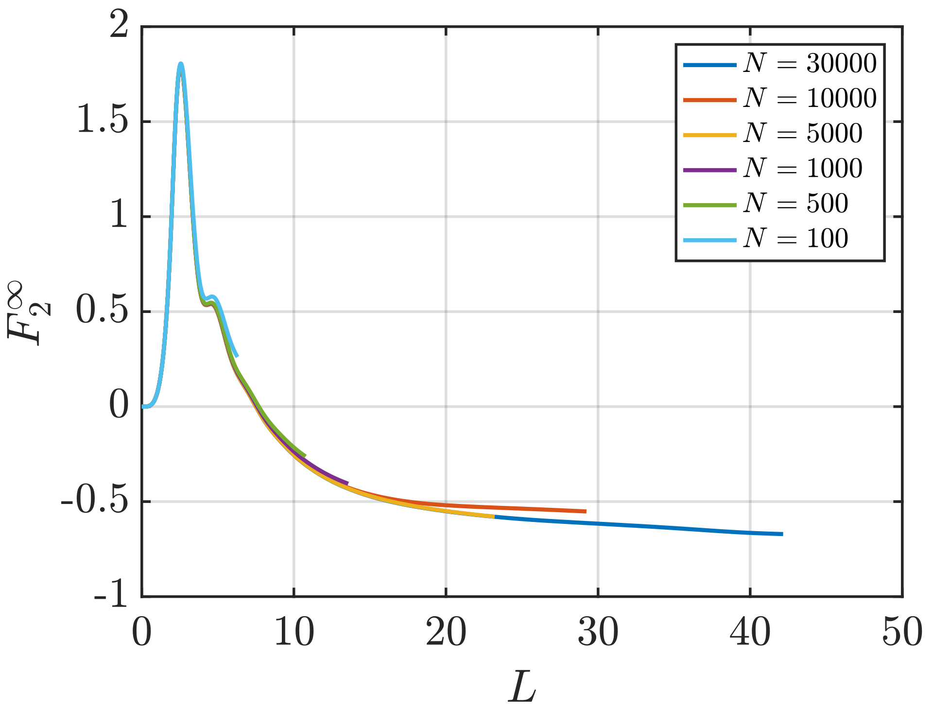
| 1. Direct estimation | (11) | A plateau in is identified when plotted as a function of L. To estimate , values of in this plateau are averaged. |
| 2. Scaling of with | (9) and (10) | To find , the slope of the linear part of the scaling is computed. |
| 3. Scaling of with | (4) and (12) | To find , the intercept of the linear part of the scaling is computed. |
| N | Scaling of with | Direct Estimation | Scaling of with L |
|---|---|---|---|
| 500 | n/a | ||
| 1000 | n/a | ||
| 5000 | |||
| 10,000 | |||
| 30,000 | |||
| 50,000 |
| N | Scaling of with | Direct Estimation | Scaling of with L |
|---|---|---|---|
| 500 | n/a | n/a | |
| 1000 | n/a | ||
| 5000 | |||
| 10,000 | |||
| 30,000 |
| N | Direct Estimation | Scaling of with L | Scaling of with L |
|---|---|---|---|
| 500 | n/a | n/a | |
| 1000 | n/a | ||
| 5000 | |||
| 10,000 | |||
| 30,000 | |||
| 50,000 |
| N | Direct Estimation | Scaling of with L | Scaling of with L |
|---|---|---|---|
| 500 | n/a | n/a | |
| 1000 | n/a | n/a | |
| 5000 | |||
| 10,000 | |||
| 30,000 |
© 2020 by the authors. Licensee MDPI, Basel, Switzerland. This article is an open access article distributed under the terms and conditions of the Creative Commons Attribution (CC BY) license (http://creativecommons.org/licenses/by/4.0/).
Share and Cite
Dawass, N.; Krüger, P.; Schnell, S.K.; Moultos, O.A.; Economou, I.G.; Vlugt, T.J.H.; Simon, J.-M. Kirkwood-Buff Integrals Using Molecular Simulation: Estimation of Surface Effects. Nanomaterials 2020, 10, 771. https://doi.org/10.3390/nano10040771
Dawass N, Krüger P, Schnell SK, Moultos OA, Economou IG, Vlugt TJH, Simon J-M. Kirkwood-Buff Integrals Using Molecular Simulation: Estimation of Surface Effects. Nanomaterials. 2020; 10(4):771. https://doi.org/10.3390/nano10040771
Chicago/Turabian StyleDawass, Noura, Peter Krüger, Sondre K. Schnell, Othonas A. Moultos, Ioannis G. Economou, Thijs J. H. Vlugt, and Jean-Marc Simon. 2020. "Kirkwood-Buff Integrals Using Molecular Simulation: Estimation of Surface Effects" Nanomaterials 10, no. 4: 771. https://doi.org/10.3390/nano10040771
APA StyleDawass, N., Krüger, P., Schnell, S. K., Moultos, O. A., Economou, I. G., Vlugt, T. J. H., & Simon, J.-M. (2020). Kirkwood-Buff Integrals Using Molecular Simulation: Estimation of Surface Effects. Nanomaterials, 10(4), 771. https://doi.org/10.3390/nano10040771