John Carroll’s Views on Intelligence: Bi-Factor vs. Higher-Order Models

Abstract

The development of factor models is inextricably tied to the history of intelligence research. One of the most commonly-cited scholars in the field is John Carroll, whose three-stratum theory of cognitive ability has been one of the most influential models of cognitive ability in the past 20 years. Nonetheless, there is disagreement about how Carroll conceptualized the factors in his model. Some argue that his model is best represented through a higher-order model, while others argue that a bi-factor model is a better representation. Carroll was explicit about what he perceived the best way to represent his model, but his writings are not always easy to understand. In this article, I clarify his position by first describing the details and implications of bi-factor and higher-order models then show that Carroll’s published views are better represented by a bi-factor model.

1. Introduction

Scholars have debated theories of cognitive ability for over a century [1]. Inextricably related to these debates are debates about the how to represent the theories in a factorial model. Arguably, Francis Galton [2] came up with the first theory of intelligence, but it was decades later before Spearman [3] developed a factorial model that represented Galton’s theory. Soon thereafter, scholars developed a variety of alternative factor models to map onto a variety of theories about the structure of cognitive ability. In fact, much of the early progress made in the development of factor analysis came from disagreements about how to measure and model cognitive ability [4,5,6].

In some respects, the debate over the “best” way to represent the structure of cognitive ability largely ended in the last part of the twentieth century following the publication of John Carroll’s [7] Human Cognitive Abilities. Google Scholar reports that this book has been cited over 5000 times. Jensen [8] wrote “It is unlikely that his monumental feat …could be much improved on. It will long be the key reference point and a solid foundation for the explanatory era of differential psychology” (p. 5), and Lubinski [9] echoed this sentiment by writing “it is among a handful of the best treatments ever published on individual differences in cognitive abilities” (p. 44). In other respects, Carroll’s work revived a century-old debate on the nature of the factors, especially general intelligence (g). Specifically, the debate centers on how to model the factors. While ostensibly, this is an esoteric issue, the implications from the different models are manifold [10]. Thus, it is important to understand Carroll’s conceptualization of cognitive ability. Carroll was explicit in his writings about what he perceived the best way to represent g, but his writings are not always easy to understand.

The purpose of this article is to help clarify Carroll’s position. I will do this by first describing the two most common competing models for representing g. Subsequently, I will discuss the substantive implications that results from each model and then use Carroll’s own published views on the best way to factorially model cognitive ability.

2. Models of Intelligence

There are a variety of factorial models designed to represent the structure of cognitive ability. Models that contain g, however, can be classified as either bi-factor or higher-order representations. While the higher-order model is technically nested within the bi-factor model [11], they provide very different conceptualizations of g and other factors in the model. Consequently, I develop the models separately. To understand both models, it is important to first understand their common predecessor: the two-factor model.

2.1. Two-Factor Model

Spearman [3] originally developed his two-factor model as a way to represent Francis Galton’s proposals [2] about cognitive ability, namely that all measures of cognitive ability have something in common: g [12]. Spearman was not really interested testing Galton’s theory, as he firmly believed that g existed by the time he started collecting the data for his study [13]. Nonetheless, the two-factor model that he developed in the process was the foundation for the development of factor analysis.

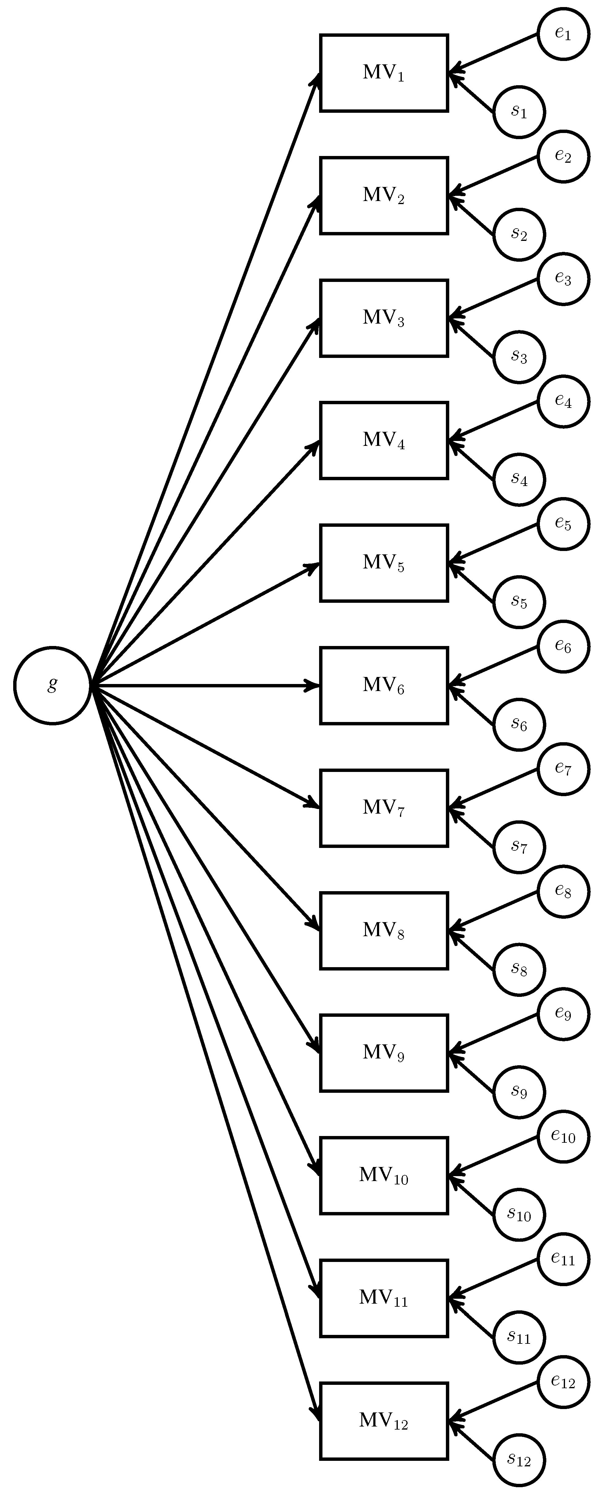
An example of a two-factor model is in Figure 1. The name of the model is a bit of a misnomer, as it contains more than two factors.1 Specifically, the model consists of: (a) g, which represents what is common to all of the measured variables (MVs); (b) specific factors (s), one for each MV, which represent systematic variance in a given MV that is unexplained by g and; (c) error (e), which represents the unsystematic (i.e., unexplained) variability in each MV [14].

Figure 1. Example of a two-factor model. MV: measured variable; s: specific factors; e: error.

Figure 1. Example of a two-factor model. MV: measured variable; s: specific factors; e: error.

There are a few things to note about this model. First, Spearman [16] distinguished s from e by applying a correction formula to the MVs’ correlations. He believed that through this correction, he could remove error from his model. This is why he called it a two-factor theory, the two factors being g and s. There are problems in using this correction [17], so typically, e and s are not separable in a factor analysis. Instead, they are combined together in a single residual factor for each MV. For didactic purposes, I keep them separate.

Second, all of the factors have a direct influence on the MVs. This direct influence of all of the factors on the MVs is an important aspect of the model that often gets overlooked. What this means is that changes in the levels of g or s directly result in changes in the values of the MVs. The factor loading is the amount of change in the MV expected from a change in a factor.

Third, all of the factors are independent of each other. Thus, changes in levels g should have no influence on any of the s factors and vice versa. Consequently, one could theoretically increase the level on any of the s factors and, subsequently, increase the values of the MVs, without affecting g.

Fourth, the model does not contain group factors, which are factors that influence a subset of the MVs. This is by design. Spearman did not deny the existence of group factors. In fact, he directed some of his students’ dissertations to focus on these factors (e.g., [18,19]), and he wrote about them extensively in some of his last publications [20,21]. Spearman just viewed most group factors as being arbitrary and resulting from including redundant MVs. Thus, he typically either used datasets where the MVs had little in common (outside of g) or pooled together scores from tests that he thought were too similar.

Not long after Spearman published his two-factor model, scholars began criticizing it (e.g., [22,23,24,25]). Criticisms tended to cluster along one of two lines: either group factors existed in addition to g and s or g was just an artifact of Spearman’s approach to collecting and analyzing data.2 Eventually, most scholars who did not deny the existence of g came to agree that Spearman’s model needed to be extended to account for group factors [5,26]. The manner in which the model should be extended, however, differed in what Carroll and Schweiker [27] called British and American approaches. The British approach is “top-down” [28]; thus, it prioritizes g and tends to treat group factors as residuals (i.e., aspects of the MVs that g cannot explain). The American approach is “bottom-up”; thus, it prioritizes group factors and either excludes g or relegates it to being the result of some datasets producing multiple correlated group factors.

2.2. Bi-Factor Model

Karl Holzinger developed the bi-factor model as an extension of the two-factor model that allows for the presence of group factors [29]. The bi in the bi-factor model refers to the two levels of common factors: general and group. Holzinger and colleagues developed the bi-factor model as part of the Unitary Trait Study at the University of Chicago [30].

Although Spearman’s name does not appear as an author on the seminal bi-factor model publications, his influence is still there. Holzinger did post-doctoral work with Spearman, from which they published on some technical aspects of the two-factor model [31,32,33]. They continued working together as part of the Unitary Trait Study, which culminated in Spearman coming to the University of Chicago as a visiting professor in order to work with Holzinger on developing the bi-factor model [35,36].

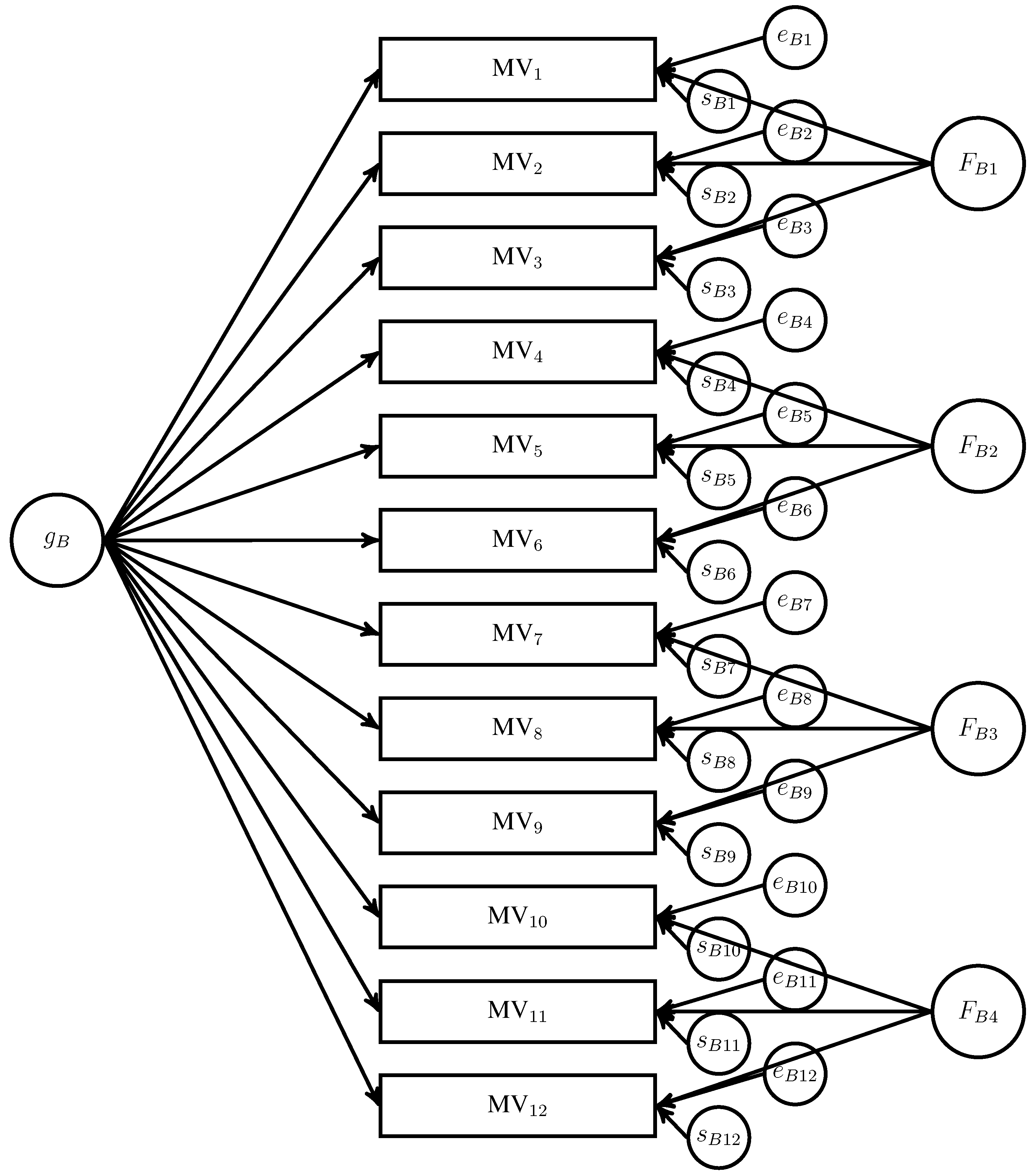
An example of a bi-factor model is in Figure 2. It has four essential parts: (a) $g_B$; (b) $s_B$; (c) $e_B$; and (d) group factors ($F_B$), with the B subscript indicating that the factor comes from a bi-factor model. Like $s_B$, $F_B$ are residual factors, because the bi-factor model requires estimating them from the covariance remaining among the MVs after accounting for $g_B$. As with the two-factor model, the bi-factor model specifies that all of the factors have a direct influence on the MVs. Thus, changes in levels of $g_B$, $F_B$ or $s_B$ directly result in changes in the expected value of the MVs. In addition, all of the factors are independent of each other.3 Thus, the influence of a change in the level of $g_B$ on the MVs is independent of any changes in levels of any other factor, and vice versa.

Originally, bi-factor models were estimated through a series of purposeful factor “extractions” that bear little resemblance to modern methods of factor analysis [29,37]. Currently, they are estimated through confirmatory factor models (sometimes called nested-factors models [28]) or analytic rotations in exploratory factor analysis [38]. Regardless of the method, however, the goal of prioritizing g over group factors has always been paramount. Thus, it is part of the British “top-down” approach to modeling intelligence.

2.3. Higher-Order Model

The higher-order model has its origins in L.L. Thurstone’s multiple factor models. Thurstone’s [39] approach to factor analysis was to focus on extracting and interpreting group factors. Interestingly, both Spearman and Thurstone thought that the factorial description of a measured variable should remain the same if the variable were moved to another battery of tests (i.e., invariance). Spearman [40] thought this was not possible at the group factor level, so he focused on g. Conversely, Thurstone did not think g was invariant, so he focused most of his work on group factors, what he called primary mental abilities [14,41].4

To find invariant group factors, Thurstone rotated any extracted factors until they met a set of criteria, what he called simple structure, that he believed optimized their generalizability across datasets [42]. Initially, the factor rotations that Thurstone used to achieve the simple structure were orthogonal [14,23], which precluded the factors from being correlated. Eventually, he came to realize that when the data come from cognitive ability measures, which tend to produce a set of correlations that are all positive and non-negligible in size, that the extracted factors should be able to correlate [43]. When he subsequently began using oblique rotations, he found that the factors were often strongly correlated with each other. Moreover, if enough group factors were present, then their correlations could be factor analyzed to find higher-order factors [45]. For cognitive ability data, the apex of this higher-order factor model often contained a single factor that he thought was equivalent to Spearman’s g [42].

Figure 2. Example of a bi-factor model. MV: measured variable; F: group factors; s: specific factors; e: error.

Figure 2. Example of a bi-factor model. MV: measured variable; F: group factors; s: specific factors; e: error.

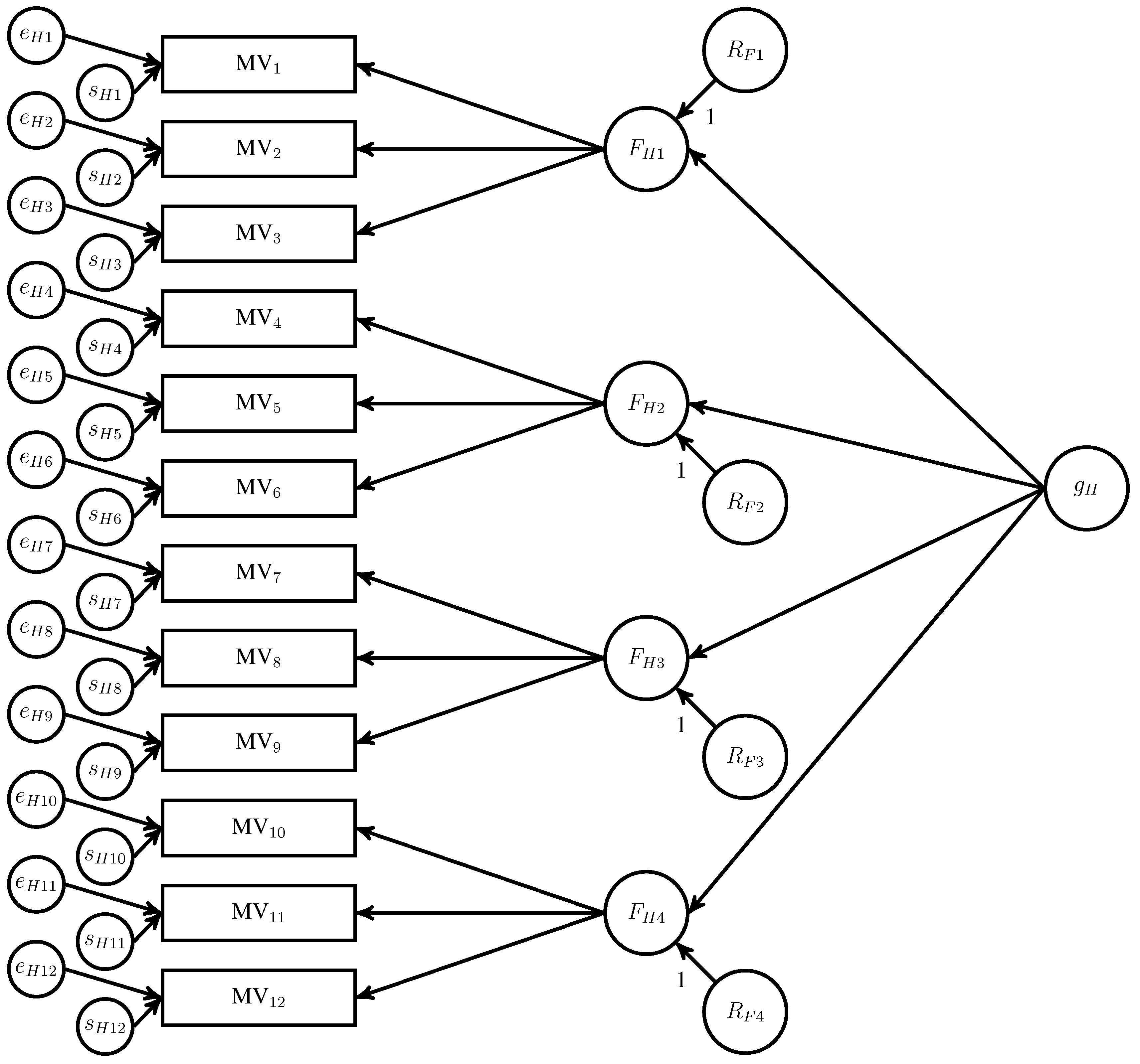
An example of a higher-order model is in Figure 3. There are five parts to the model: (a) $g_H$; (b) $s_H$; (c) $e_H$; (d) $F_H$; and (e) group residuals (R), with the H subscript indicating the factor comes from a higher-order model.5 The group residuals are present because of the way $g_H$ is formed. In the higher-order model, the shared variance among the MVs is only used to form $F_H$; it does not contribute to the formation of $g_H$. Consequently, $F_H$ are formed first and have the highest priority. This is why higher-order models align with the American “bottom-up” approach of prioritizing group factors over g [46].

Figure 3. Example of a higher-order factor model. MV: measured variable; F: group factors; s: specific factors; e: error; R: group factor residuals.

Figure 3. Example of a higher-order factor model. MV: measured variable; F: group factors; s: specific factors; e: error; R: group factor residuals.

In higher-order models, $F_H$ are expected to account for all of the MVs’ common variance. Any systematic variance in the MVs not explained by $F_H$ is captured by $s_H$. If there are enough $F_H$ and they share enough variance, $g_H$ can be formed from $F_H$.6 Thus, $g_H$ is only expected to account for the common variance among the $F_H$. Any variance in $F_H$ not explained by $g_H$ is captured by R. Because R are residual terms, they are all uncorrelated with each other, as well as $g_H$, $s_H$ and $e_H$.

2.4. Implications from the Models about the Nature of Cognitive Ability

Higher-order models of cognitive ability were Thurstone’s [42] way of reconciling his initial primary factor model and Spearman’s two-factor model. While both models contain g, F and s factors, the models, as well as the factors formed from them, are not interchangeable.

First, and perhaps the most substantive difference, is how the models represent g’s relation to the MVs [48]. In the bi-factor model, g has a direct influence on the MVs; so, a change in $g_B$ results in an expected change in the MVs of the magnitude and size of MV’s factor loading on $g_B$. In higher-order models, g does not have a direct influence on the MVs. Instead, $g_H$’s influence on the MV is indirect, working through $F_H$. In other words, $g_H$’s relation to the MVs is fully mediated by $F_H$. Thus, a change in the level of $g_H$ only results in a change in $F_H$; it is the change in $F_H$ that produces any changes in the levels of the MVs. MacKinnon, Fairchild and Fritz [49] described additional implications of having a mediation model.

Second, the very nature of g differs between the models. In bi-factor models, the major difference between g and F is the breadth of MVs that they influence [50]. By its nature, $g_B$ influences a substantially larger breadth of MVs than $F_B$. In contrast, higher-order models differentiate g and F through their order. $g_H$ is a super-ordinate factor, so it is of a higher order than $F_H$. Consequently, $g_H$ subsumes $F_H$.

Third, the composition of F differs between the models. In bi-factor models, $F_B$ reflect what is common among a group of MVs after accounting for $g_B$. Thus, $F_B$ are independent of $g_B$. In higher-order models, $F_H$ reflect what is common among a subset of MVs. Only if there are enough $F_H$ that share a sufficient amount of common variance can $g_H$ be formed. If $g_F$ is formed, then $F_H$ can be partitioned into what they all have in common (i.e., $g_H$) and what is unique (i.e., R).

As $F_B$ and R are both residuals, it is easy to conclude that they are essentially interchangeable. This is not necessarily the case. $g_B$ is formed directly from the MVs, and then, $F_B$ are extracted from whatever residual covariance remains among the MVs. In contrast, $F_H$ are formed directly from the MVs, and $g_H$ is formed from $F_H$. As $g_H$ is estimated only from what is common among $F_H$, R represents what is unique to a given group factor from all of the other group factors. Unless the $F_H$ can perfectly reproduce the MVs’ correlations, $g_B$ and $g_H$ are formed from different sets of variable relationships, so they will be different; this then makes the group-level residuals—R and $F_B$—different. The extent of the difference between $g_B$ and $g_H$, and subsequently $F_B$ and R, will depend on the dataset used for the analysis.

Fourth, related to the differences in F between the models is the difference in how g and F relate to each other. In a bi-factor model, $F_B$ are formed from any covariance among the MVs that remains after forming $g_B$. Consequently, $g_B$ and $F_B$ are independent of each other. A change in $g_B$ does not produce any changes in $F_B$, and vice versa. In higher-order models, $g_H$ and $F_H$ are not independent. Thurstone [42] noted as much, saying that $g_H$ is a “participant in the definition of” $F_H$ (p. 418). The reasons for this dependence are a little complex [51,52]. Conceptually, the dependence of $F_H$ and $g_H$ can be seen by noting that the loadings of $F_H$ on $g_H$ are just a re-expression of the correlations among $F_H$ [53].

While the difference among the F–g relations between the bi-factor and higher-order models may be important in developing theories of cognitive ability, the implications of these differences really come to bear when other variables are included in the model that relate to both F and g. This is often done in the study of academic achievement [54] or aging [52]. Using external variables with $g_B$ and $F_B$ does not pose a problem, because the factors are all independent of each other. Using external variables with $g_H$ and $F_H$, however, can produce a situation where the predictor variables are linearly dependent on each other, or at least related enough to cause problems with multicollinearity (e.g., [55]).

2.5. Schmid–Leiman Transformation

In 1957, John Schmid and John Leiman [56] published a way to transform loadings from a higher-order factor model to emphasize the relations among the MVs and factors—specifically $g_H$ and R—to aid in factor interpretation. There was nothing exceptionally novel about Schmid and Leiman’s method, as the relationships could be calculated individually using what is now called tracing rules [57]. The major contribution of Schmid and Leiman’s transformation (SLT) of higher-order factor loadings is that it does the calculations for all MVs simultaneously.

At the time of this article, there are almost 700 references to Schmid and Leiman’s article [56] on Google Scholar. Some historical context is needed to understand the popularity of the SLT. Like Spearman’s original method, Holzinger’s method for estimating bi-factor loadings looks almost nothing like what is currently thought of as factor analysis. It does not require any iteration process or factor rotation; in fact, it can be done through hand calculations [34]. While Spearman thought highly of Holzinger’s method as a way to account for g and group factors concurrently [20], it largely fell out of favor in the middle of the twentieth century. Factor analysts, especially in America, largely ignored British models [58] and focused their attention on developing more robust ways to extract and rotate group factors. Psychologists largely turned their attention away from factor analysis, per se, towards trying to understand the underlying processes involved in the different aspects of cognitive ability. Jensen [4] wrote:

By the mid-1940s, the factor analysis of abilities had about run its course in its potential conceptual contribution to the study of human intelligence. From the viewpoint of theoretical development, the whole field went into the doldrums for nearly a quarter of a century. Strictly methodological and statistical developments and refinements in factor analysis and test theory came to occupy the center stage, whereas the substantive issues of differential psychology remained virtually at an impasse.

(p. 81)

Those interested in studying g typically did so using the first unrotated factor from an exploratory factor analysis (or the simpler principal components analysis) or used a higher-order factor analysis. Those who still wished to use a bi-factor model to conceptualize cognitive ability were primarily relegated to either using confirmatory factor analysis or approximating a bi-factor model using the SLT of a higher-order model [59].

Until the recent development of analytic bi-factor rotations [38,60], it made sense to substitute the SLT of a higher-order model for a bi-factor model when conducting an exploratory factor analysis [61]. Traditional estimation of bi-factor loadings does not make use of all of the methodological advances made in factor analysis, and the SLT produces results that often appear to mimic a bi-factor model since R and g are uncorrelated. As I described in Section 2.4, however, bi-factor and higher-order models are not equivalent. As the SLT just re-expresses the factor loadings from a higher-order factor model in a form that highlights the relation of the MVs to g and R, the resulting loadings from the SLT are still estimates derived from a higher-order model [53].

3. John Carroll’s Model of Human Cognitive Abilities

Having described higher-order and bi-factor models, it is now possible to describe John Carroll’s views on intelligence, or at least the factor model that should represent it. Carroll’s study of human intelligence coincided with his study of factor-analysis, all of which started while he was a graduate student and was able to visit the University of Chicago to study with Thurstone. After he graduated in 1940, he had a distinguished career producing many publications that contributed to the literature in a variety of fields. It was largely after he started his work on Human Cognitive Abilities, however, when he began to write about his theory of cognitive ability and the factor model he thought best represented it.

Carroll’s [7] most well-known work in intelligence is his seminal book in which he reanalyzed over 460 datasets containing measures of cognitive ability published from 1930 to 1985. From his meta-analytic work, Carroll developed a three-stratum theory of intelligence. This theory postulates that all factors resulting from the analysis of cognitive ability measures can be classified as being at one of three strata, which refer to the levels of the factors’ abstractness [62].

Factors at Stratum I are the least abstract and can often be determined from the test content. Some examples are induction, numerical facility and visualization. Factors at Stratum II are more general, and thus more abstract, than those at Stratum I, so typically, they cannot be determined by test content alone. Stratum II factors are equivalent to the group factors that I discussed throughout this article. Some examples are fluid intelligence and crystallized intelligence. At Stratum III, there is only one factor: g. It is the most abstract and most general factor in Carroll’s theory.

Many have interpreted Carroll’s work as supporting a higher-order model (e.g., [63,64]). For example, Murray and Johnson [65] wrote “there are no explicitly or implicitly bi-factor theories of intelligence” (p. 419). Likewise, Reynolds and Keith [66] wrote “we believe that higher-order models are theoretically more defensible, more consistent with relevant intelligence theory …, than are less constrained (bi-factor) models” (p. 66). While there may be support favoring a higher-order model over a bi-factor model, it is not correct to attribute Carroll’s work as supporting this notion. Although sometimes his writing is not easy to understand, Carroll was explicit in noting that a bi-factor model best represents his theory.

First, Carroll [47] considered Spearman’s work to be an “honorable first approximation” to his three stratum theory. Spearman’s [67] conceptualization of g was that:

Every performance depends partly on some common fund of energy. This, then, is the required General Factor. …Every performance depends, not only on this General Factor, but also in varying degree on a factor specific to itself and all very similar performances …Every intellectual act appears to involve, both the specific activity of a particular system of cortical neurons, and also the general energy of the whole cortex.

(p. 79)

In other words, Spearman believed that g was directly involved in all cognitive “performances”, not indirectly involved through, or mediated by, other factors. This stands in dire contrast to Thurstone’s conceptualization [42] of g as a super-ordinate factor whose primary purpose was to help define group factors.

Spearman did not write about group factors much except to note that most of them were substantively unimportant. When he did examine group factors (e.g., [68]), he conceptualized them as resulting from variance in common between two or more s factors:

…all such large multiplication of [group] factors in an ability does not arise from renouncing its primary and fundamental bisection into the original two factors, universal [g] and the non-universal [s]; it only comes from submitting the non-universal factor to further and secondary sub-division.

([40], p. 599)

Note Spearman’s conceptual equating of specific and group factors. Thus, as specific factors stem from variance in the MVs that g could not explain and are independent of g, so, too, are group factors.

While he disagreed with Spearman’s idea that g represents a “common fund of energy”, Carroll largely agreed with Spearman’s conceptualization [67] of g as having a direct, not indirect, influence on MVs and being independent of any group factors.

A general factor of intelligence is one that would exhibit significantly positive loadings on all, or nearly all, the individual difference variables that could be selected or devised in the total domain of cognitive abilities, whether or not the loadings are accompanied by loadings on lower-order factors in this domain. Further, it is required that the general factor is independent of any factors and constitutes a “true ability”, as could be defined by relevant operations … it would be desirable to show also that a general factor so identified constitutes a true ability, independent of lower-order factors, rather than being merely a measure of associations among those lower-order factors that might be due, for example, to the effects of common learnings.

([69], pp. 143–144)

To my mind, (orthogonal) factors represent latent causal elements in test scores. For example,…a variable with a loading of 0.6 on a general factor, 0.5 on a fluid intelligence factor at Stratum II, a loading of 0.4 on a Stratum I verbal factor and a loading of 0.3 on a Stratum I induction factor, could be assumed to be independently influenced by each of those factors, to the extent indicated by the loadings.

([47], p. 4)

The idea that g and group factors operate directly and separately is echoed in Carroll’s [70,71] model of learning. He postulated that there were two kinds of cognitive factors that govern how much time an individual would need to learn something. The first is the ability to understand instruction, which is g or some amalgam of g and verbal ability. The second is aptitude, which consists of one or more specific abilities (i.e., group factors) that are required for a given task. He considered these two aspects to work relatively independently of each other, as the ability to understand instruction could directly overcome some environmental problems, such as poor instruction.

Second, at the time he did the analysis for Human Cognitive Abilities, Carroll wanted to use a bi-factor model. Due to the number of datasets he had to analyze and the lack of computational power available on most computers when he was doing his analyses (mid-1980s), he decided to only use exploratory factor analyses (EFA) [7]. At that time, an analytic bi-factor rotation was not available, so he chose to conduct a higher-order EFA and then to transform all of the loadings using the SLT. He did this because he thought the procedure would form “an orthogonal factor pattern very similar to the Spearman–Holzinger bi-factor pattern” ([7], p. 90). Nonetheless, Carroll was aware of the drawbacks stemming from this approach. He [72] wrote:

To a degree, I believe that the Schmid–Leiman procedure … constitutes a straitjacket because it assumes that factors at a given order subsume factors at a lower order, as indicated by the correlations among those lower-order factors. This assumption may not be correct; the true situation may merely be that factors differ in generality of application, without subsumptions such that a loading on a second-order factor implies a loading on some one of a particular set of first-order factors.

(p. 47)

Later, Carroll lamented only using EFA for his book’s analyses, as confirmatory factor analysis (CFA) was better able to model a bi-factor structure than EFA. In the 1980s, however, CFA procedures were just too difficult and computationally expensive to perform for all of the many datasets he had accumulated. After his book was published, in at least three separate publications [69,73,74], he used CFA to model his three-stratum theory. In all of the CFA models, he represented his theory using a bi-factor model.

Third, one could argue that in most of the figures he made to represent his three-stratum theory, Carroll used a higher-order model. Carroll [47] cautions that these figures “should not be taken too literally or precisely” (p. 4). Instead, underlying these figures:

…at another level of presentation, so to speak, one can assume a structure of orthogonal …factors that differ principally in their generality over the domain of cognitive abilities. The g factor is most general, second-stratum factors are less general, and first-stratum factors are least general. Actually one can envisage a structure in which all factors are orthogonal, differing only in their degree of generality.

(p. 4)

4. Discussion

John Carroll’s contributions to psychology are manifold [9]. The importance of his Human Cognitive Abilities book [7] probably cannot be overstated. It is arguably one of the most influential works in the history of intelligence research [75] and “will be found on the bookshelves of scholars of the subject for decades” ([9], p. 44). Thus, it is important to understand Carroll’s views on intelligence accurately, or at least the model that he believed best represents his view.

Throughout his writings, John Carroll described his view of cognitive ability as: (a) comprising multiple influences (factors), each of which are independent of each other; (b) the influences differing in their level of generality over the entire domain of cognitive ability; (c) the most general influence, g, having an direct relation to all, or nearly all, possible measures of cognitive ability and; (d) g existing independently of group factors. All desiderata map directly onto a bi-factor model, not a higher-order model.

This is not to say that a bi-factor model accurately represents the structure of cognitive ability or that Carroll’s work is without flaw [76]. Like all models, Carroll’s is likely wrong in certain aspects. The veracity of the model aside, it will likely continue to serve as a foundation for the study of cognitive ability in the foreseeable future. Consequently, his model should be represented accurately, which is best done through a bi-factor model.

References

1. Thorndike, R.L.; Lohman, D. A Century of Ability Testing; Riverside Publishing: Chicago, IL, USA, 1990. [Google Scholar]
2. Galton, F. Introduction Into Human Faculty and Its Development; AMS Press: New York, NY, USA, 1883. [Google Scholar]
3. Spearman, C.E. “General intelligence”, objectively determined and measured. Am. J. Psychol. 1904, 15, 201–293. [Google Scholar] [CrossRef]
4. Jensen, A.R. Individual differences in mental ability. In Historical Foundations of Educational Psychology; Glover, J.A., Ronning, R.R., Eds.; Plenum Press: New York, NY, USA, 1987; pp. 61–88. [Google Scholar]
5. Carroll, J.B. The measurement of intelligence. In Handbook of Human Intelligence; Sternberg, R.J., Ed.; Cambridge University Press: New York, NY, USA, 1982; pp. 29–120. [Google Scholar]
6. Thorndike, R.M. History of factor analysis: A psychological perspective. In Encyclopedia of Statistics in Behavioral Science; Everitt, B.S., Howell, D.C., Eds.; John Wiley: Hoboken, NJ, USA, 2005; Volume 2, pp. 842–851. [Google Scholar]
7. Carroll, J.B. Human Cognitive Abilities: A Survey of Factor-Analytic Studies; Cambridge University Press: New York, NY, USA, 1993. [Google Scholar]
8. Jensen, A.R. Obituary: John Bissell Carroll. Intelligence 2004, 32, 1–5. [Google Scholar] [CrossRef]
9. Lubinski, D. John Bissell Carroll (1916–2003). Am. Psychol. 2004, 59, 43–44. [Google Scholar] [CrossRef] [PubMed]
10. Brunner, M. No g in education? Learn. Individ. Differ. 2008, 18, 152–165. [Google Scholar] [CrossRef]
11. Yung, Y.F.; Thissen, D.; McLeod, L.D. On the relationship between the higher-order factor model and the hierarchical factor model. Psychometrika 1999, 64, 113–128. [Google Scholar] [CrossRef]
12. Spearman, C.E. A History of Psychology in Autobiography; Murchison, C., Ed.; Clark University Press: Worcester, MA, USA, 1930; Volume 1, pp. 229–333. [Google Scholar]
13. Bartholomew, D.J. Spearman and the origin and development of factor analysis. Br. J. Math. Stat. Psychol. 1995, 48, 211–220. [Google Scholar] [CrossRef]
14. Thurstone, L.L. The vectors of mind. Psychol. Rev. 1934, 41, 1–32. [Google Scholar] [CrossRef]
15. Bollen, K.A. Latent variables in psychology and the social sciences. Ann. Rev. Psychol. 2002, 53, 605–634. [Google Scholar] [CrossRef] [PubMed]
16. Spearman, C.E. The proof and measurement of association between two things. Am. J. Psychol. 1904, 15, 72–101. [Google Scholar] [CrossRef]
17. Muchinsky, P.M. The correction for attenuation. Educ. Psychol. Meas. 1996, 56, 63–75. [Google Scholar] [CrossRef]
18. McFarlane, M.M. A Study of Practical Ability; The Cambridge University Press: Cambridge, UK, 1925; Volume 8. [Google Scholar]
19. El Koussy, A.A.H. An Investigation Into the Factors in Tests Involving the Visual Perception of Space; The Cambridge University Press: Cambridge, UK, 1935; Volume 20. [Google Scholar]
20. Spearman, C.E.; Wynn Jones, L. Human Ability: A Continuation of “The Abilities of Man”; Macmillan: London, UK, 1950; p. 198. [Google Scholar]
21. Spearman, C.E. Theory of general factor. Br. J. Psychol. 1946, 36, 117–131. [Google Scholar]
22. Thorndike, E.L.; Lay, W.; Dean, P.R. The relation of accuracy in sensory discrimination to general intelligence. Am. J. Psychol. 1909, 20, 364–369. [Google Scholar] [CrossRef]
23. Thurstone, L.L. Multiple factor analysis. Psychol. Rev. 1931, 38, 406–427. [Google Scholar] [CrossRef]
24. Thomson, G.H. General versus group factors in mental activities. Psychol. Rev. 1920, 27, 173–190. [Google Scholar] [CrossRef]
25. Garnett, J.C.M. On certain independent factors in mental measurements. Proc. R. Soc. Lond. Ser. A 1919, 96, 91–111. [Google Scholar] [CrossRef]
26. Wolfle, D. Factor analysis to 1940. Psychom. Monogr. 1940, 3, 69. [Google Scholar]
27. Carroll, J.B.; Schweiker, R.F. Factor analysis in educational research. Rev. Educ. Res. 1951, 21, 368–388. [Google Scholar] [CrossRef]
28. Gustafsson, J.E.; Balke, G. General and specific abilities as predictors of school achievement. Multivar. Behav. Res. 1993, 28, 407–434. [Google Scholar] [CrossRef]
29. Holzinger, K.J.; Swineford, F. The bi-factor method. Psychometrika 1937, 2, 41–54. [Google Scholar] [CrossRef]
30. Holzinger, K.J. Recent research on unitary mental traits. J. Personal. 1936, 4, 335–343. [Google Scholar] [CrossRef]
31. Spearman, C.E.; Holzinger, K. The average value for the probable error of tetrad differences. Br. J. Psychol. Gen. Sec. 1930, 20, 368–370. [Google Scholar] [CrossRef]
32. Spearman, C.E.; Holzinger, K. Note on the sampling error of tetrad differences. Br. J. Psychol. Gen. Sec. 1925, 16, 86–88. [Google Scholar] [CrossRef]
33. Spearman, C.E.; Holzinger, K.J. The sampling error in the theory of two factors. Br. J. Psychol. 1924, 15, 17–19. [Google Scholar] [CrossRef]
34. Wherry, R.J. Contributions to Correlational Analysis; Academic Press: Orlando, FL, USA, 1984. [Google Scholar]
35. Harman, H.H. Karl John Holzinger. Psychometrika 1954, 19, 95–96. [Google Scholar] [CrossRef]
36. Holzinger, K.J. Spearman as I knew him. Psychometrika 1945, 10, 231–235. [Google Scholar] [CrossRef] [PubMed]
37. Holzinger, K.J.; Harman, H.H. Comparison of two factorial analyses. Psychometrika 1938, 3, 45–60. [Google Scholar] [CrossRef]
38. Jennrich, R.I.; Bentler, P. Exploratory bi-factor analysis. Psychometrika 2011, 76, 537–549. [Google Scholar] [CrossRef] [PubMed]
39. Thurstone, L.L. Current issues in factor analysis. Psychol. Bull. 1940, 37, 189–236. [Google Scholar] [CrossRef]
40. Spearman, C.E. The factor theory and its troubles. III. Misrepresentation of the theory. J. Educ. Psychol. 1933, 24, 591–601. [Google Scholar] [CrossRef]
41. Thurstone, L.L. Primary mental abilities. Psychom. Monogr. 1938, 1, 121. [Google Scholar]
42. Thurstone, L.L. Multiple Factor Analysis; University of Chicago Press: Chicago, IL, USA, 1947. [Google Scholar]
43. Thurstone, L.L. A new rotational method in factor analysis. Psychometrika 1938, 3, 199–218. [Google Scholar] [CrossRef]
44. Rindskopf, D.; Rose, T. Some theory and applications of confirmatory second-order factor analysis. Multivar. Behav. Res. 1988, 23, 51–67. [Google Scholar] [CrossRef]
45. Thurstone, L.L. Second-order factors. Psychometrika 1944, 9, 71–100. [Google Scholar] [CrossRef]
46. Gustafsson, J.E. On the hierarchical structure of ability and personality. In Intelligence and Personality: Bridging the Gap in Theory And Measurement; Collis, J.M., Messick, S., Eds.; Lawrence Erlbaum: Mahwah, NJ, USA, 2001; pp. 25–42. [Google Scholar]
47. Carroll, J.B. A three-stratum theory of intelligence: Spearman’s contribution. In Human Abilities: Their Nature and Measurement; Dennis, I., Tapsfield, P., Eds.; Lawrence Erlbaum: Mahwah, NJ, USA, 1996; pp. 1–17. [Google Scholar]
48. Tucker, L.R. The role of correlated factors in factor analysis. Psychometrika 1940, 5, 141–152. [Google Scholar] [CrossRef]
49. MacKinnon, D.P.; Fairchild, A.J.; Fritz, M.S. Mediation analysis. Ann. Rev. Psychol. 2007, 58, 593–614. [Google Scholar] [CrossRef] [PubMed]
50. Gignac, G.E. Higher-order models versus direct hierarchical models: g as superordinate or breadth factor? Psychol. Sci. Q. 2008, 50, 21–43. [Google Scholar]
51. Rijmen, F. Formal relations and an empirical comparison among the bi-factor, the testlet, and a second-order multidimensional IRT model. J. Educ. Meas. 2010, 47, 361–372. [Google Scholar] [CrossRef]
52. Schmiedek, F.; Li, S.C. Toward an alternative representation for disentangling age-associated differences in general and specific cognitive abilities. Psychol. Aging 2004, 19, 40–56. [Google Scholar] [CrossRef] [PubMed]
53. Reise, S.P. The rediscovery of bifactor measurement models. Multivar. Behav. Res. 2012, 47, 667–696. [Google Scholar] [CrossRef] [PubMed]
54. McGrew, K.S.; Wendling, B.J. Cattell-Horn-Carroll cognitive-achievement relations: What we have learned from the past 20 years of research. Psychol. Sch. 2010, 47, 651–675. [Google Scholar] [CrossRef]
55. Beaujean, A.A.; Parkin, J.; Parker, S. Comparing Cattell-Horn-Carroll models for predicting language achievement: Differences between bi-factor and higher-order factor models. Psychol. Assess. 2014, 26, 789–805. [Google Scholar] [CrossRef] [PubMed]
56. Schmid, J.; Leiman, J. The development of hierarchical factor solutions. Psychometrika 1957, 22, 53–61. [Google Scholar] [CrossRef]
57. Boker, S.M.; McArdle, J.J.; Neale, M. An Algorithm for the Hierarchical Organization of Path Diagrams And Calculation of Components of Expected Covariance. Struct. Equ. Modeling 2002, 9, 174–194. [Google Scholar] [CrossRef]
58. Mulaik, S.A. Factor analysis and Psychometrika: Major developments. Psychometrika 1986, 51, 23–33. [Google Scholar] [CrossRef]
59. Jensen, A.R.; Weng, L.J. What is a good g? Intelligence 1994, 18, 231–258. [Google Scholar] [CrossRef]
60. Reise, S.P.; Moore, T.M.; Haviland, M.G. Bifactor models and rotations: Exploring the extent to which multidimensional data yield univocal scale scores. J. Personal. Assess. 2010, 92, 544–559. [Google Scholar] [CrossRef] [PubMed]
61. Carroll, J.B. Exploratory factor analysis: A tutorial. In Current Topics in Human Intelligence; Detterman, D., Ed.; Ablex Publishing Corp.: Norwood, NJ, USA, 1985; Volume 1, pp. 25–58. [Google Scholar]
62. Carroll, J.B. The three-stratum theory of cognitive abilities. In Contemporary Intellectual Assessment, 3rd ed.; Flanagan, D.P., Harrison, P.L., Eds.; Guilford: New York, NY, USA, 2012; pp. 883–890. [Google Scholar]
63. Schneider, W.J.; McGrew, K.S. The Cattell-Horn-Carroll model of intelligence. In Contemporary Intellectual Assessment, 3rd ed.; Flanagan, D.P., Harrison, P.L., Eds.; Guilford: New York, NY, USA, 2012; pp. 99–144. [Google Scholar]
64. Kaufman, S.B.; Reynolds, M.R.; Liu, X.; Kaufman, A.S.; McGrew, K.S. Are cognitive g and academic achievement g one and the same g? An exploration on the Woodcock–Johnson and Kaufman tests. Intelligence 2012, 40, 123–138. [Google Scholar] [CrossRef]
65. Murray, A.L.; Johnson, W. The limitations of model fit in comparing the bi-factor versus higher-order models of human cognitive ability structure. Intelligence 2013, 41, 407–422. [Google Scholar] [CrossRef]
66. Reynolds, M.R.; Keith, T.Z. Measurement and statistical issues in child assessment research. In The Oxford Handbook of Child Psychological Assessment; Saklofske, D.H., Schwean, V.L., Reynolds, C.R., Eds.; Oxford University Press: New York, NY, USA, 2013; pp. 48–83. [Google Scholar]
67. Hart, B.; Spearman, C. General ability, its existance and nature. Br. J. Psychol. 1912, 5, 51–84. [Google Scholar]
68. Spearman, C.E. Thurstone’s work re-worked. J. Educ. Psychol. 1939, 30, 1–16. [Google Scholar] [CrossRef]
69. Carroll, J.B. Theoretical and technical issues in identifying a factor of general intelligence. In Intelligence, Genes, and Success: Scientists Respond to The Bell Curve; Devlin, B., Fienberg, S.E., Resnick, D.P., Roeder, K., Eds.; Springer-Verlag: New York, NY, USA, 1997; pp. 125–156. [Google Scholar]
70. Carroll, J.B. A model of school learning. Teach. Coll. Rec. 1963, 64, 723–733. [Google Scholar]
71. Carroll, J.B. The prediction of success in intensive foreign language training. In Training Research and Education; Glaser, R., Ed.; University of Pitsburgh Press: Pittsburgh, PA, USA, 1962; pp. 87–136. [Google Scholar]
72. Carroll, J.B. Factor analysis since Spearman: Where do we stand? What do we know. In Abilities, Motivation, and Methodology: The Minnesota Symposium on Learning and Individual Differences; Kanfer, R., Ackerman, P.L., Cudeck, R., Eds.; Routledge: New York, NY, USA, 1989; Volume 10, pp. 43–70. [Google Scholar]
73. Carroll, J.B. On methodology in the study of cognitive abilities. Multivar. Behav. Res. 1995, 30, 429–452. [Google Scholar] [CrossRef]
74. Carroll, J.B. The higher-stratum structure of cognitive abilities: Current evidence supports g and about ten broad factors. In The Scientific Study of General Intelligence: Tribute to Arthur R. Jensen; Nyborg, H., Ed.; Pergamon: New York, NY, USA, 2003; pp. 5–21. [Google Scholar]
75. McGrew, K.S. CHC theory and the human cognitive abilities project: Standing on the shoulders of the giants of psychometric intelligence research. Intelligence 2009, 37, 1–10. [Google Scholar] [CrossRef]
76. Horn, J.L.; McArdle, J.J. Understanding human intelligence since Spearman. In Factor Analysis at 100; Cudeck, R., MacCallum, R.C., Eds.; Lawrence Erlbaum: Mahwah, NJ, USA, 2007; pp. 205–247. [Google Scholar]
• 1.Some would not consider the specific or error components of the model to be factors. In fact, Thurstone [14] called Spearman’s model a single-factor model, as he thought it only represented a single latent variable (i.e., g). Following Bollen [15], I refer to them as factors.
• 2.Spearman’s “test” for the number of factors (i.e., tetrad differences) and method for estimating factor loadings look little like current methods in factor analysis (see Wherry [34] for a didactic example).
• 3.There are bi-factor models that allow the group factors to correlate with each other [44], but they are seldom used, so I do not discuss them.
• 4.Bartholomew [13] and Carroll and Schweiker [27] noted that, mathematically, there really was not much difference between Spearman’s and Thurstone’s approach to factor analysis. The main difference lay in the their interpretations of what was more psychological meaningful: g or group factors; although even here, their two approaches were not inconsistent with each other.
• 5.Technically, the factors from the higher-order model are not equivalent to those in bi-factor models. I use the same name for the factors in each model, however, following John Carroll’s presentations of the models (e.g., [47]).
• 6.Having enough group factors available to estimate higher-order factors is not an inconsequential problem. Carroll [7] (pp. 89–90) noted that many studies of cognitive ability (at least those published before 1985) did not collect enough variables to form a sufficient number of group factors for a robust estimate of g using a higher-order model.