Enhancing Spatial Ability Assessment: Integrating Problem-Solving Strategies in Object Assembly Tasks Using Multimodal Joint-Hierarchical Cognitive Diagnosis Modeling


Abstract
1. Introduction
1.1. Facets of Spatial Ability
1.2. Problem-Solving Strategy
1.3. Traditional and Objective Measures of Problem-Solving
1.4. Multimodal Assessments
1.5. Research Questions
2. Materials and Methods
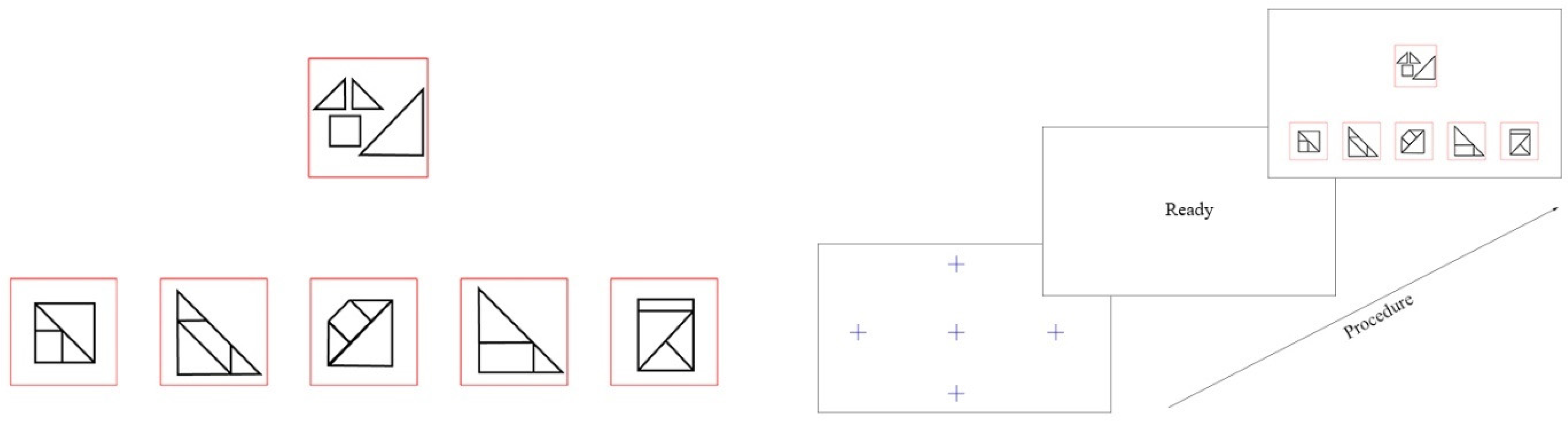
2.1. Instrument
2.2. Sample
2.3. Procedure
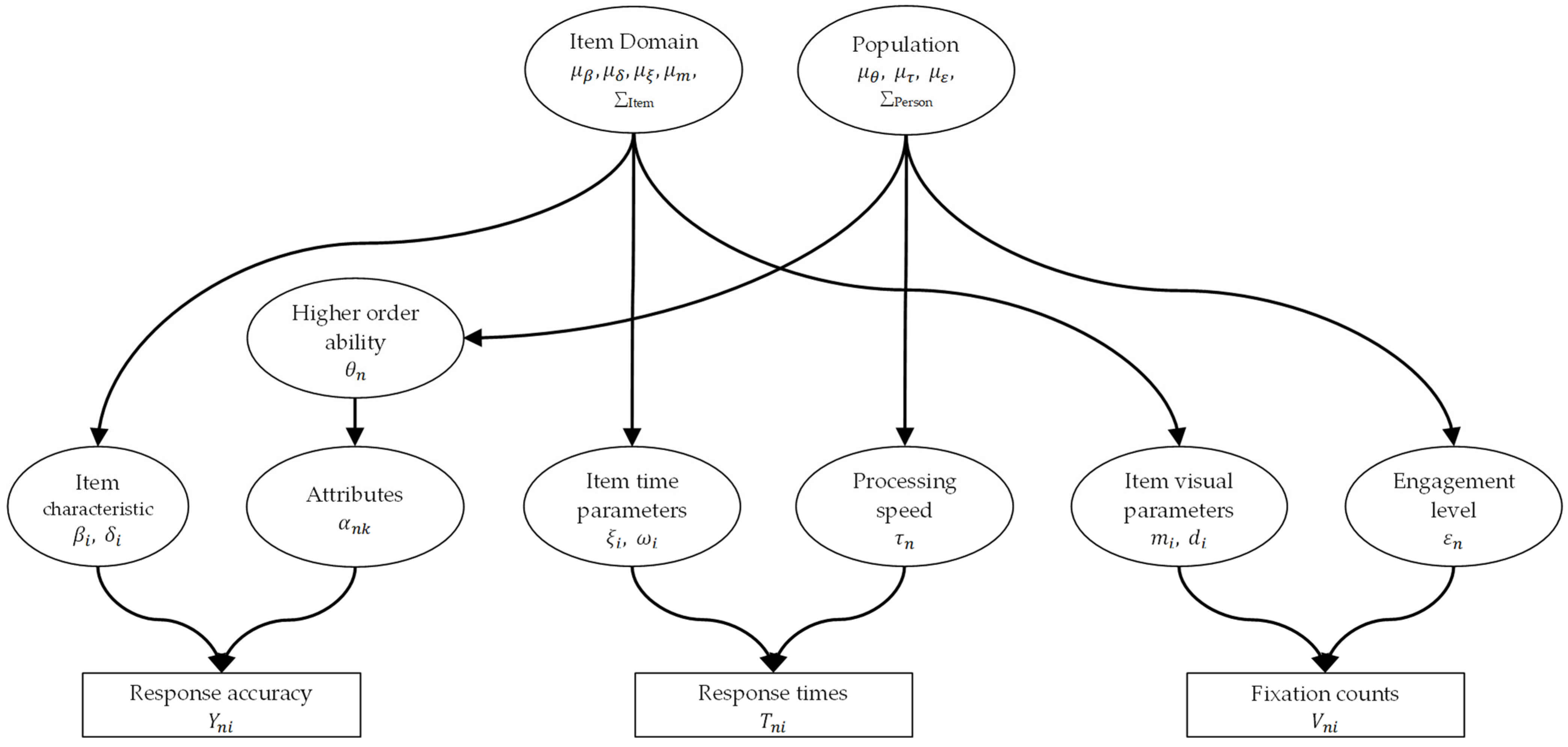
2.4. Model
2.4.1. The Higher-Order DINA Model
2.4.2. The Lognormal RT Model
2.4.3. The Negative Binomial Fixation (NBF) Model
2.4.4. Assumptions
2.4.5. Bayesian Estimation
2.4.6. Coding
3. Results
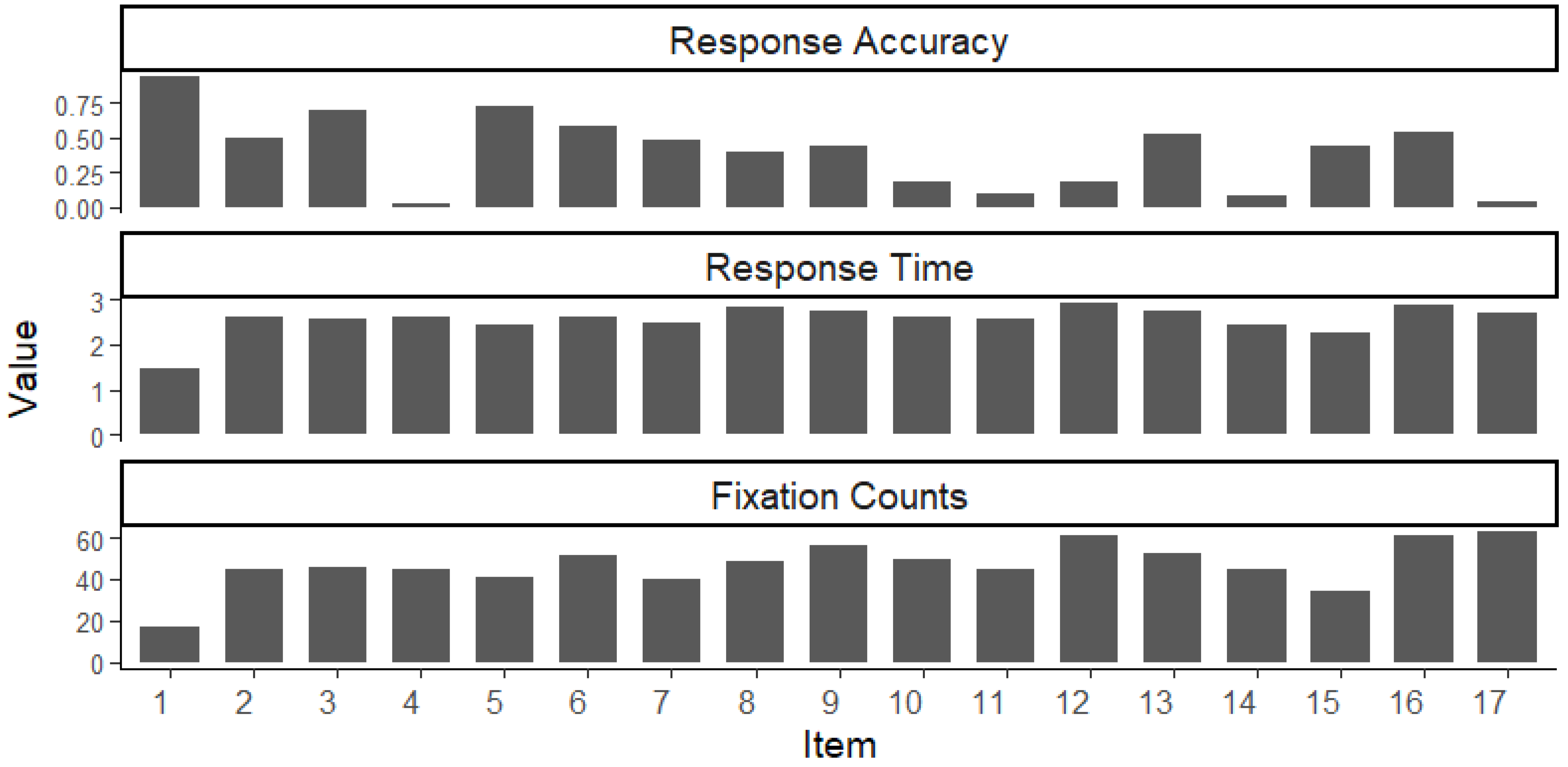
3.1. Data Description and Analysis
3.2. Result of MJ-DINA Model
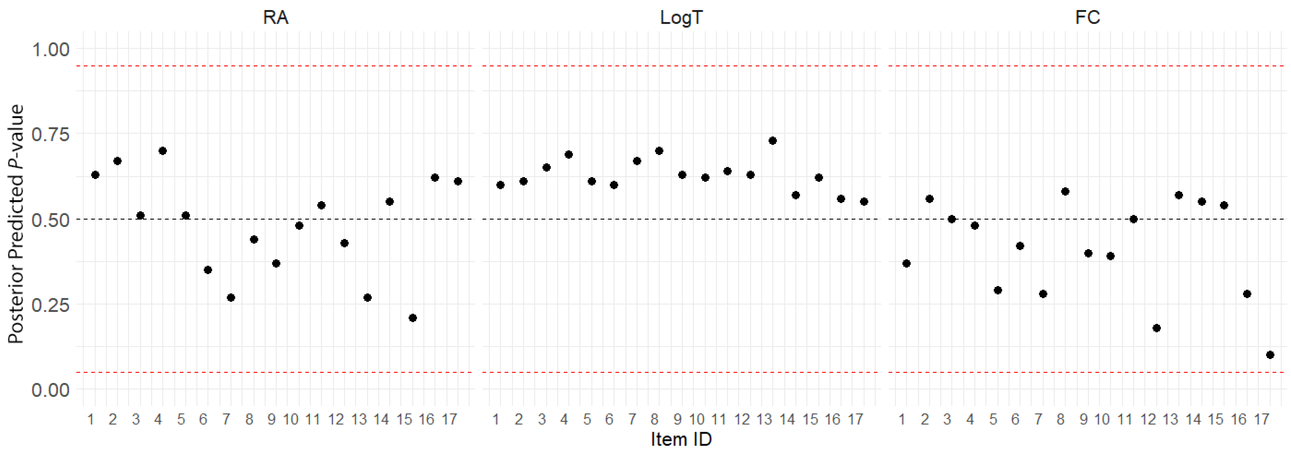
3.2.1. Convergence Diagnostics and Model Fit
3.2.2. Relationship Between MJ-DINA Parameters
3.2.3. Item Parameter Estimation
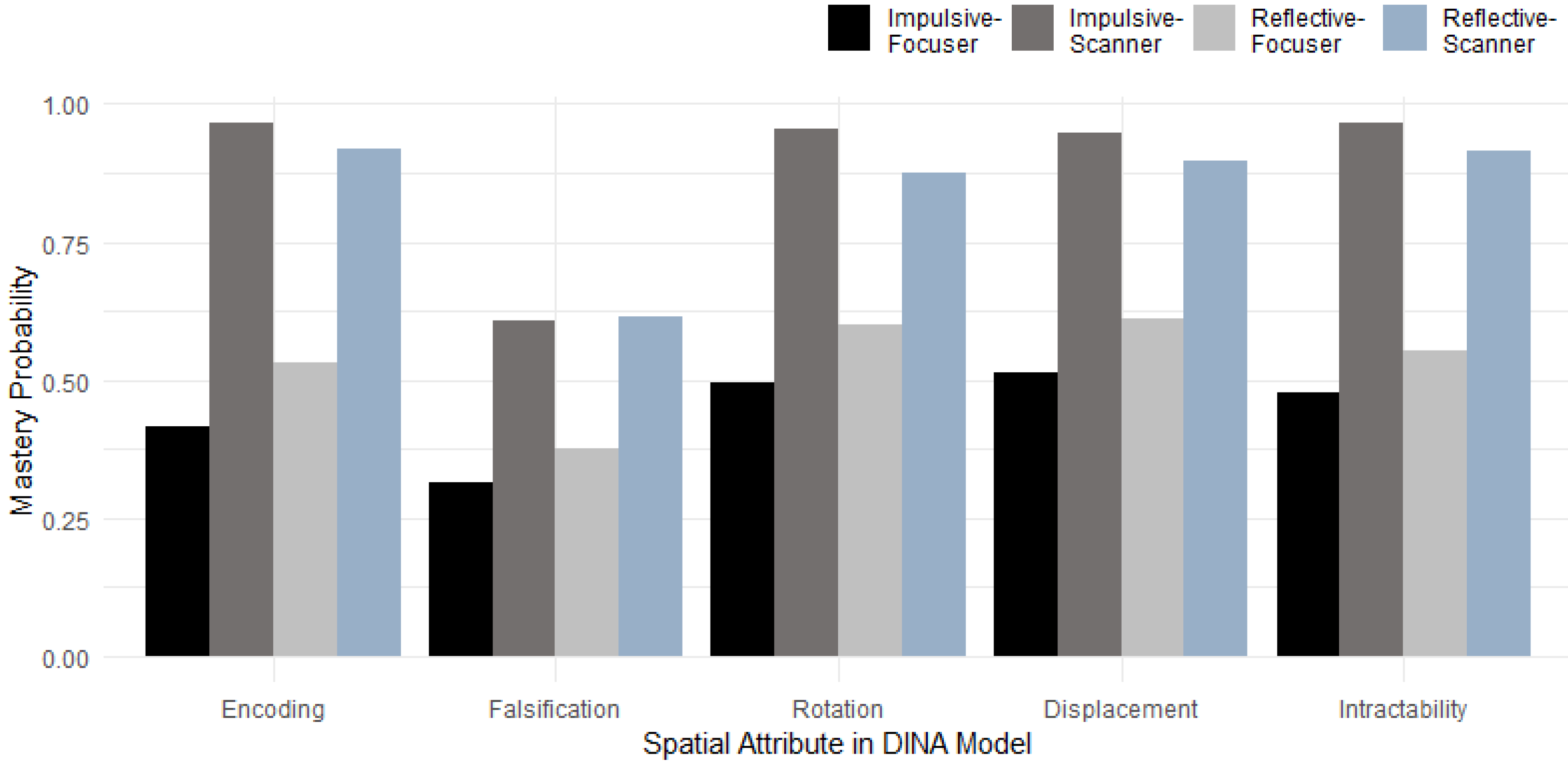
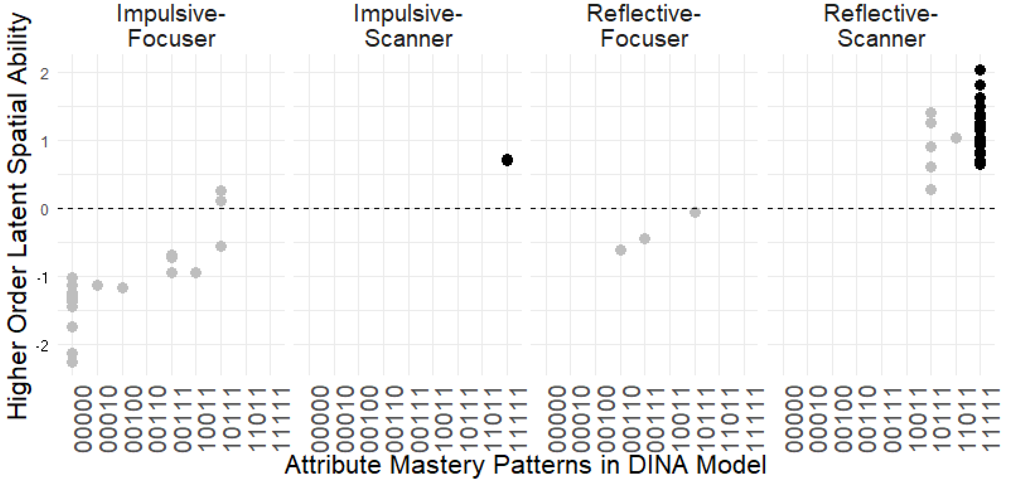
3.3. Inferring Spatial Strategies from DINA Estimates
4. Discussion
4.1. Research Question 1
4.2. Research Question 2
4.3. Research Question 3
5. Conclusions
5.1. Implications
5.2. Limitations
5.3. Future Research
Author Contributions
Funding
Institutional Review Board Statement
Informed Consent Statement
Data Availability Statement
Conflicts of Interest
References
- Ackerman, Phillip L., and Ruth Kanfer. 2009. Test length and cognitive fatigue: An empirical examination of effects on performance and test-taker reactions. Journal of Experimental Psychology: Applied 15: 163–81. [Google Scholar] [CrossRef] [PubMed]
- Anderson, Charles H., David C. Van Essen, and Bruno A. Olshausen. 2005. Directed visual attention and the dynamic control of information flow. In Neurobiology of Attention. Cambridge: Academic Press, pp. 11–17. [Google Scholar] [CrossRef]
- Bornstein, Robert F. 2011. Toward a process-focused model of test score validity: Improving psychological assessment in science and practice. Psychological Assessment 23: 532. [Google Scholar] [CrossRef]
- Brooks, Stephen P., and Andrew Gelman. 1998. General methods for monitoring convergence of iterative simulations. Journal of Computational and Graphical Statistics 7: 434–55. [Google Scholar] [CrossRef]
- Carroll, John Bissell. 1993. Human Cognitive Abilities: A Survey of Factor-Analytic Studies. Cambridge: Cambridge University Press. [Google Scholar] [CrossRef]
- Cooper, Lynn A., and Roger N. Shepard. 1973. Chronometric studies of the rotation of mental images. In Visual Information Processing. Cambridge: Academic Press, pp. 75–176. [Google Scholar] [CrossRef]
- Curtis, S. McKay, Ilya Goldin, and Evangelos Evangelou. 2015. mcmcplots: Create Plots from MCMC Output. Available online: https://CRAN.R-project.org/package=mcmcplots (accessed on 2 March 2024).
- De La Torre, Jimmy. 2011. The Generalized DINA Model Framework. Psychometrika 76: 179–99. [Google Scholar] [CrossRef]
- De La Torre, Jimmy, and Jeffrey A. Douglas. 2004. Higher-order latent trait models for cognitive diagnosis. Psychometrika 69: 333–53. [Google Scholar] [CrossRef]
- Embretson, Susan, and Joanna Gorin. 2001. Improving construct validity with cognitive psychology principles. Journal of Educational Measurement 38: 343–68. [Google Scholar] [CrossRef]
- Gardner, Riley W., Philip S. Holzman, George S. Klein, Harriet P. Linton, and Donald P. Spence. 1959. Cognitive control: A study of individual consistencies in cognitive behavior. Psychological Issues 1: 1–186. [Google Scholar]
- Gelman, Andrew, Xiao-Li Meng, and Hal Stern. 1996. Posterior predictive assessment of model fitness via realized discrepancies. Statistica Sinica 6: 733–60. [Google Scholar]
- Gorin, Joanna S. 2006. Test design with cognition in mind. Educational Measurement: Issues and Practice 25: 21–35. [Google Scholar] [CrossRef]
- Haertel, Edward H. 1989. Using restricted latent class models to map the skill structure of achievement items. Journal of Educational Measurement 26: 301–21. [Google Scholar] [CrossRef]
- Halpern, Diane F. 2000. Sex Differences in Cognitive Abilities. London: Psychology Press. [Google Scholar] [CrossRef]
- Hawes, Zachary, and Daniel Ansari. 2020. What explains the relationship between spatial and mathematical skills? A review of evidence from brain and behavior. Psychonomic Bulletin & Review 27: 465–82. [Google Scholar] [CrossRef]
- Heil, Martin, and Petra Jansen-Osmann. 2008. Sex differences in mental rotation with polygons of different complexity: Do men utilize holistic processes whereas women prefer piecemeal ones? Quarterly Journal of Experimental Psychology 61: 683–89. [Google Scholar] [CrossRef]
- Holmqvist, Kenneth, Marcus Nyström, Richard Andersson, Richard Dewhurst, Halszka Jarodzka, and Joost Van de Weijer. 2011. Eye Tracking: A Comprehensive Guide to Methods and Measures. Oxford: Oxford University Press. [Google Scholar]
- Höffler, Tim N. 2010. Spatial ability: Its influence on learning with visualizations—A meta-analytic review. Educational Psychology Review 22: 245–69. [Google Scholar] [CrossRef]
- Ihaka, Ross, and Rober Gentleman. 1996. R: A language for data analysis and graphics. Journal of Computational and Graphical Statistics 5: 299–314. [Google Scholar] [CrossRef]
- Jäkel, Frank, Manish Singh, Felix A. Wichmann, and Michael. H. Herzog. 2016. An overview of quantitative approaches in Gestalt perception. Vision Research 126: 3–8. [Google Scholar] [CrossRef]
- Just, Marcel A., and Patricia A. Carpenter. 1976. Eye fixations and cognitive processes. Cognitive Psychology 8: 441–80. [Google Scholar] [CrossRef]
- Kagan, Jerome. 1965. Reflection-impulsivity and reading ability in primary grade children. Child Development 36: 609–28. [Google Scholar] [CrossRef]
- Kail, Rober, Philip Carter, and James Pellegrino. 1979. The locus of sex differences in spatial ability. Perception & Psychophysics 26: 182–86. [Google Scholar] [CrossRef]
- Kanamori, Nobuhiro, and Akihiro Yagi. 2002. The difference between flipping strategy and spinning strategy in mental rotation. Perception 31: 1459–66. [Google Scholar] [CrossRef]
- Kirschner, Paul A. 2017. Stop propagating the learning styles myth. Computers & Education 106: 166–71. [Google Scholar] [CrossRef]
- Kozhevnikov, Maria, Mary Hegarty, and Richard E. Mayer. 2002. Revising the visualizer-verbalizer dimension: Evidence for two types of visualizers. Cognition and Instruction 20: 47–77. [Google Scholar] [CrossRef]
- Kyllonen, Patrick C., and Raymond E. Christal. 1990. Reasoning ability is (little more than) working-memory capacity? Intelligence 14: 389–433. [Google Scholar] [CrossRef]
- Lam, Chi-Ming. 2007. Is Popper’s falsificationist heuristic a helpful resource for developing critical thinking? Educational Philosophy and Theory 39: 432–48. [Google Scholar] [CrossRef]
- Linn, Marcia C., and Anne C. Petersen. 1985. Emergence and Characterization of Sex Differences in Spatial Ability: A Meta-Analysis. Child Development 56: 1479–98. [Google Scholar] [CrossRef] [PubMed]
- Liu, Yaohui, Peida Zhan, Yanbin Fu, Qipeng Chen, Kaiwen Man, and Yikun Luo. 2023. Using a multi-strategy eye-tracking psychometric model to measure intelligence and identify cognitive strategy in Raven’s advanced progressive matrices. Intelligence 100: 101782. [Google Scholar] [CrossRef]
- Lohman, David. F. 1979. Spatial Ability: A Review and Reanalysis of the Correlational Literature. Stanford: School of Education, Stanford University. [Google Scholar]
- Lohman, David. F. 1996. Spatial Ability and g. In Human Abilities. London: Psychology Press. [Google Scholar]
- Man, Kaiwen, and Jeffrey R. Harring. 2019. Negative binomial models for visual fixation counts on test items. Educational and Psychological Measurement 79: 617–35. [Google Scholar] [CrossRef]
- Man, Kaiwen, Jeffrey R. Harring, and Peida Zhan. 2022. Bridging models of biometric and psychometric assessment: A three-way joint modeling approach of item responses, response times, and gaze fixation counts. Applied Psychological Measurement 46: 361–81. [Google Scholar] [CrossRef]
- Maris, Eric. 1999. Estimating multiple classification latent class models. Psychometrika 64: 187–212. [Google Scholar] [CrossRef]
- McGee, Mark G. 1979. Human spatial abilities: Psychometric studies and environmental, genetic, hormonal, and neurological influences. Psychological Bulletin 86: 889. [Google Scholar] [CrossRef]
- Mitchell, Tom M., Paul E. Utgoff, and Ranan Banerji. 1983. Learning by experimentation: Acquiring and refining problem-solving heuristics. Machine Learning: An Artificial Intelligence Approach I: 163–90. [Google Scholar] [CrossRef]
- Miyake, Akira, and Priti Shah. 1999. Models of Working Memory. Cambridge: Cambridge University Press, pp. 422–81. [Google Scholar] [CrossRef]
- Miyake, Akira, Naomi P. Friedman, David A. Rettinger, Priti Shah, and Mary Hegarty. 2001. How are visuospatial working memory, executive functioning, and spatial abilities related? A latent-variable analysis. Journal of Experimental Psychology: General 130: 621. [Google Scholar] [CrossRef]
- Nazareth, Alina, Rebecca Killick, Anthony S. Dick, and Shannon M. Pruden. 2019. Strategy selection versus flexibility: Using eye-trackers to investigate strategy use during mental rotation. Journal of Experimental Psychology: Learning, Memory, and Cognition 45: 232–45. [Google Scholar] [CrossRef] [PubMed]
- Nickerson, Raymond S. 1998. Confirmation bias: A ubiquitous phenomenon in many guises. Review of General Psychology 2: 175–220. [Google Scholar] [CrossRef]
- Nuttall, Ronald L., M. Beth Casey, and Elizabeth Pezaris. 2005. Spatial Ability as a Mediator of Gender Differences on Mathematics Tests: A Biological-Environmental Framework. Cambridge: Cambridge University Press. [Google Scholar] [CrossRef]
- Pellegrino, James W., Randall J. Mumaw, and Valerie J. Shute. 1985. Analyses of spatial aptitude and expertise. In Test Design. Cambridge: Academic Press, pp. 45–76. [Google Scholar] [CrossRef]
- Petrova, Kate, and James J. Gross. 2023. The future of emotion regulation research: Broadening our field of view. Affective Science 4: 609–16. [Google Scholar] [CrossRef] [PubMed]
- Plummer, Martyn. 2017. JAGS Version 4.3. 0 User Manual. Available online: https://sourceforge.net/projects/mcmc-jags/files/Manuals/4.x/ (accessed on 2 March 2024).
- Plummer, Martyn. 2023. JAGS: Just Another Gibbs Sampler. Available online: https://mcmc-jags.sourceforge.io (accessed on 2 March 2024).
- Plummer, Martyn, Nicky Best, Kate Cowles, and Karen Vines. 2006. CODA: Convergence diagnosis and output analysis for MCMC. R News 6: 7–11. [Google Scholar]
- Popper, Karl R. 1963. Science as falsification. Conjectures and Refutations 1: 33–39. [Google Scholar]
- Quasha, William H., and Rensis Likert. 1937. The revised Minnesota paper form board test. Journal of Educational Psychology 28: 197–204. [Google Scholar] [CrossRef]
- Ramful, Ajay, Thomas Lowrie, and Tracy Logan. 2017. Measurement of spatial ability: Construction and validation of the spatial reasoning instrument for middle school students. Journal of Psychoeducational Assessment 35: 709–27. [Google Scholar] [CrossRef]
- Reilly, David, and David L. Neumann. 2013. Gender-role differences in spatial ability: A meta-analytic review. Sex Roles 68: 521–35. [Google Scholar] [CrossRef]
- Salhi, Saïd. 2017. Heuristic Search: The Emerging Science of Problem Solving. Cham: Palgrave Macmillan. [Google Scholar] [CrossRef]
- Serbin, Lisa A., Phyllis Zelkowitz, Anna-Beth Doyle, Dolores Gold, and Blair Wheaton. 1990. The socialization of sex-differentiated skills and academic performance: A mediational model. Sex Roles 23: 613–28. [Google Scholar] [CrossRef]
- Shepard, Roger N. 1978. The mental image. American Psychologist 33: 125. [Google Scholar] [CrossRef]
- Shepard, Roger N., and Jacqueline Metzler. 1971. Mental rotation of three-dimensional objects. Science 171: 701–3. [Google Scholar] [CrossRef]
- Sternberg, Robert J., and Elena L. Grigorenko. 1997. Are cognitive styles still in style? American Psychologist 52: 700. [Google Scholar] [CrossRef]
- Sternberg, Robert J., and Scott Barry Kaufman. 2011. The Cambridge Handbook of Intelligence. Cambridge: Cambridge University Press. [Google Scholar] [CrossRef]
- Thurstone, Louis Leon, and Thelma Gwinn Thurstone. 1941. Factorial studies of intelligence. Psychometric Monographs 2: 94. [Google Scholar]
- Unkelbach, Christian. 2006. The learned interpretation of cognitive fluency. Psychological Science 17: 339–45. [Google Scholar] [CrossRef]
- Uttal, David H., Nathaniel G. Meadow, Elizabeth Tipton, Linda L. Hand, Alison R. Alden, Christopher Warren, and Nora S. Newcombe. 2013. The malleability of spatial skills: A meta-analysis of training studies. Psychological Bulletin 139: 352. [Google Scholar] [CrossRef] [PubMed]
- Van der Linden, Wim J. 2006. A lognormal model for response times on test items. Journal of Educational and Behavioral Statistics 31: 181–204. [Google Scholar] [CrossRef]
- Venables, W. N., and D. M. Smith. 2003. The R development core team. An Introduction to R. Available online: https://cran.r-project.org/doc/manuals/r-devel/R-intro.html (accessed on 2 March 2024).
- Wagemans, Johan, Jacob Feldman, Sergei Gepshtein, Ruth Kimchi, James R. Pomerantz, Peter A. Van der Helm, and Cees Van Leeuwen. 2012. A century of Gestalt psychology in visual perception: II. Conceptual and theoretical foundations. Psychological Bulletin 138: 1218. [Google Scholar] [CrossRef]
- Wai, Jonathan. 2022. Spatial thinkers receive their due. Science 377: 1497. [Google Scholar] [CrossRef]
- Wai, Jonathan, and Frank C. Worrell. 2016. Helping disadvantaged and spatially talented students fulfill their potential: Related and neglected national resources. Policy Insights from the Behavioral and Brain Sciences 3: 122–28. [Google Scholar] [CrossRef]
- Wai, Jonathan, David Lubinski, and Camilla P. Benbow. 2009. Spatial ability for STEM domains: Aligning over 50 years of cumulative psychological knowledge solidifies its importance. Journal of Educational Psychology 101: 817–35. [Google Scholar] [CrossRef]
- Wang, Yingxu, and Vincent Chiew. 2010. On the cognitive process of human problem solving. Cognitive Systems Research 11: 81–92. [Google Scholar] [CrossRef]
- Yilmaz, Işık. 2009. Landslide susceptibility mapping using frequency ratio, logistic regression, artificial neural networks and their comparison: A case study from Kat landslides (Tokat—Turkey). Computers & Geosciences 35: 1125–38. [Google Scholar] [CrossRef]
- Zhan, Peida, Hong Jiao, and Dandan Liao. 2018. Cognitive diagnosis modelling incorporating item response times. British Journal of Mathematical and Statistical Psychology 71: 262–86. [Google Scholar] [CrossRef] [PubMed]
- Zhan, Peida, Hong Jiao, Kaiwen Man, and Lijun Wang. 2019. Using JAGS for Bayesian cognitive diagnosis modeling: A tutorial. Journal of Educational and Behavioral Statistics 44: 473–503. [Google Scholar] [CrossRef]
- Zhan, Peida, Kaiwen Man, Stefanie A. Wind, and Jonathan Malone. 2022. Cognitive diagnosis modeling incorporating response times and fixation counts: Providing comprehensive feedback and accurate diagnosis. Journal of Educational and Behavioral Statistics 47: 736–76. [Google Scholar] [CrossRef]


| Author | Spatial Cognitive Processes | |||
|---|---|---|---|---|
| Cooper and Shepard (1973) | Encoding | Mental Rotation | Confirmation | Motor Response |
| Pellegrino et al. (1985) | Falsification | Mental Rotation | Verification | |
| Embretson and Gorin (2001) | Encoding | Falsification | Confirmation | |
| No. | Stage | Description |
|---|---|---|
| A1 | Encoding | More than three pieces, curved edges, and standard shapes (e.g., circle, triangle). |
| A2 | Falsification | Distractors with obvious mismatches (e.g., wrong number of pieces, sizes, shapes). |
| A3 | Confirmation-Rotation | The confirmation stage for rotation depends on the number of rotated pieces. |
| A4 | Confirmation-Displacement | At least two pieces must be substantially moved into place for the correct answer |
| A5 | Confirmation-Intractability | Distractors only ruled out by subtle mismatches, requiring attention to small angular disparities. |
| Item | EN | FA | C-R | C-D | C-I |
|---|---|---|---|---|---|
| 1 | 1 | 0 | 1 | 0 | 1 |
| 2 | 1 | 0 | 1 | 1 | 1 |
| 3 | 1 | 0 | 1 | 1 | 1 |
| 4 | 0 | 0 | 1 | 0 | 1 |
| 5 | 0 | 1 | 1 | 0 | 1 |
| 6 | 1 | 1 | 1 | 1 | 1 |
| 7 | 0 | 0 | 1 | 1 | 1 |
| 8 | 1 | 0 | 1 | 0 | 1 |
| 9 | 1 | 0 | 0 | 0 | 1 |
| 10 | 0 | 0 | 1 | 1 | 1 |
| 11 | 1 | 1 | 1 | 0 | 1 |
| 12 | 1 | 1 | 1 | 1 | 1 |
| 13 | 1 | 1 | 1 | 0 | 1 |
| 14 | 1 | 0 | 1 | 0 | 1 |
| 15 | 1 | 1 | 1 | 1 | 1 |
| 16 | 1 | 0 | 0 | 1 | 1 |
| 17 | 1 | 0 | 0 | 1 | 1 |
| Item | ||||||
|---|---|---|---|---|---|---|
| 1 | 1.00 | 1.08 | 1.00 | 1.01 | 1.01 | 1.01 |
| 2 | 1.02 | 1.00 | 1.01 | 1.01 | 1.01 | 1.01 |
| 3 | 1.02 | 1.02 | 1.02 | 1.01 | 1.01 | 1.01 |
| 4 | 1.02 | 1.08 | 1.02 | 1.05 | 1.01 | 1.01 |
| 5 | 1.02 | 1.09 | 1.03 | 1.01 | 1.01 | 1.01 |
| 6 | 1.03 | 1.05 | 1.03 | 1.01 | 1.01 | 1.01 |
| 7 | 1.02 | 1.02 | 1.02 | 1.00 | 1.01 | 1.01 |
| 8 | 1.03 | 1.01 | 1.03 | 1.00 | 1.01 | 1.01 |
| 9 | 1.01 | 1.01 | 1.01 | 1.00 | 1.01 | 1.01 |
| 10 | 1.06 | 1.04 | 1.03 | 1.00 | 1.01 | 1.01 |
| 11 | 1.03 | 1.17 | 1.03 | 1.03 | 1.01 | 1.01 |
| 12 | 1.03 | 1.02 | 1.03 | 1.00 | 1.01 | 1.01 |
| 13 | 1.04 | 1.04 | 1.04 | 1.03 | 1.01 | 1.01 |
| 14 | 1.04 | 1.06 | 1.02 | 1.01 | 1.00 | 1.01 |
| 15 | 1.02 | 1.02 | 1.01 | 1.02 | 1.01 | 1.01 |
| 16 | 1.02 | 1.01 | 1.01 | 1.01 | 1.00 | 1.01 |
| 17 | 1.04 | 1.09 | 1.03 | 1.02 | 1.00 | 1.00 |
| Item | Variance–Covariance Parameter | Person | Variance–Covariance Parameter | ||
|---|---|---|---|---|---|
| Mean | CI | Mean | CI | ||
| 1.699 | (0.482, 3.313) | 2.387 | (1.004, 4.498) | ||
| 2.983 | (0.143, 9.759) | 0.253 | (0.148, 0.365) | ||
| 0.181 | (0.072, 0.318) | 0.194 | (0.114, 0.282) | ||
| 0.145 | (0.060, 0.261) | −0.532 | (−1.030, −0.116) | ||
| 1.582 | (−0.001, 4.001) | 0.467 | (0.102, 0.896) | ||
| −0.243 | (−0.607, 0.036) | −0.195 | (−0.288, −0.115) | ||
| −0.207 | (−0.518, 0.056) | ||||
| −0.209 | (−0.773, 0.191) | ||||
| −0.184 | (−0648, 0.186) | ||||
| 0.087 | (0.005, 0.192) | ||||
| Model | DINA (RA) | Log RT | NBF (FC) | |||
|---|---|---|---|---|---|---|
| Item | ||||||
| 1 | 1.82 (0.57) | 3.77 (1.61) | 0.85 (0.07) | 0.01 (0.02) | 1.46 (0.12) | 2.83 (0.10) |
| 2 | −0.77 (0.38) | 1.94 (0.59) | 0.32 (0.08) | 0.25 (0.10) | 2.55 (0.11) | 3.63 (0.09) |
| 3 | 0.02 (0.38) | 2.29 (0.75) | 0.51 (0.09) | 0.11 (0.06) | 2.52 (0.11) | 3.71 (0.09) |
| 4 | −2.92 (0.70) | −1.16 (1.13) | 0.06 (0.04) | 0.97 (0.03) | 2.58 (0.10) | 3.69 (0.10) |
| 5 | 0.34 (0.44) | 2.55 (1.15) | 0.58 (0.10) | 0.09 (0.07) | 2.38 (0.11) | 3.60 (0.10) |
| 6 | −0.16 (0.37) | 1.85 (0.94) | 0.46 (0.09) | 0.20 (0.12) | 2.59 (0.11) | 3.75 (0.10) |
| 7 | −0.70 (0.37) | 1.11 (0.55) | 0.34 (0.08) | 0.40 (0.11) | 2.44 (0.10) | 3.56 (0.09) |
| 8 | −1.07 (0.35) | 1.23 (0.49) | 0.26 (0.07) | 0.46 (0.10) | 2.77 (0.10) | 3.82 (0.09) |
| 9 | −0.97 (0.37) | 1.17 (0.49) | 0.28 (0.07) | 0.45 (0.09) | 2.71 (0.11) | 3.87 (0.10) |
| 10 | −1.68 (0.44) | 0.30 (0.61) | 0.17 (0.05) | 0.79 (0.08) | 2.58 (0.11) | 3.76 (0.10) |
| 11 | −2.11 (0.44) | −0.39 (1.13) | 0.11 (0.04) | 0.89 (0.08) | 2.52 (0.11) | 3.70 (0.09) |
| 12 | −1.64 (0.36) | 0.29 (0.70) | 0.17 (0.05) | 0.77 (0.12) | 2.85 (0.11) | 3.96 (0.10) |
| 13 | −0.41 (0.37) | 1.67 (0.93) | 0.40 (0.09) | 0.26 (0.15) | 2.71 (0.10) | 3.85 (0.08) |
| 14 | −2.18 (0.51) | −0.57 (0.92) | 0.11 (0.04) | 0.92 (0.05) | 2.41 (0.12) | 3.71 (0.11) |
| 15 | −0.56 (0.33) | 0.86 (0.76) | 0.37 (0.07) | 0.44 (0.16) | 2.24 (0.11) | 3.43 (0.10) |
| 16 | −0.76 (0.39) | 1.94 (0.60) | 0.32 (0.08) | 0.25 (0.10) | 2.80 (0.12) | 3.95 (0.11) |
| 17 | −2.66 (0.57) | −0.79 (1.04) | 0.07 (0.04) | 0.95 (0.04) | 2.69 (0.13) | 3.88 (0.12) |
| Category | N | |||
|---|---|---|---|---|
| Impulsive-Focuser (I-F) | 19 | −1.09 (0.63) | 0.46 (0.23) | −0.41 (0.22) |
| Impulsive-Scanner (I-S) | 2 | 0.72 (0.01) | 0.03 (0.03) | 0.02 (0.00) |
| Reflective-Focuser (R-F) | 3 | −0.37 (0.28) | −0.04 (0.06) | −0.05 (0.03) |
| Reflective-Scanner (R-S) | 26 | 1.11 (0.39) | −0.41 (0.24) | 0.37 (0.21) |
Disclaimer/Publisher’s Note: The statements, opinions and data contained in all publications are solely those of the individual author(s) and contributor(s) and not of MDPI and/or the editor(s). MDPI and/or the editor(s) disclaim responsibility for any injury to people or property resulting from any ideas, methods, instructions or products referred to in the content. |
© 2025 by the authors. Licensee MDPI, Basel, Switzerland. This article is an open access article distributed under the terms and conditions of the Creative Commons Attribution (CC BY) license (https://creativecommons.org/licenses/by/4.0/).
Share and Cite
Li, J.; Man, K.; Lakin, J.M. Enhancing Spatial Ability Assessment: Integrating Problem-Solving Strategies in Object Assembly Tasks Using Multimodal Joint-Hierarchical Cognitive Diagnosis Modeling. J. Intell. 2025, 13, 30. https://doi.org/10.3390/jintelligence13030030
Li J, Man K, Lakin JM. Enhancing Spatial Ability Assessment: Integrating Problem-Solving Strategies in Object Assembly Tasks Using Multimodal Joint-Hierarchical Cognitive Diagnosis Modeling. Journal of Intelligence. 2025; 13(3):30. https://doi.org/10.3390/jintelligence13030030
Chicago/Turabian StyleLi, Jujia, Kaiwen Man, and Joni M. Lakin. 2025. "Enhancing Spatial Ability Assessment: Integrating Problem-Solving Strategies in Object Assembly Tasks Using Multimodal Joint-Hierarchical Cognitive Diagnosis Modeling" Journal of Intelligence 13, no. 3: 30. https://doi.org/10.3390/jintelligence13030030
APA StyleLi, J., Man, K., & Lakin, J. M. (2025). Enhancing Spatial Ability Assessment: Integrating Problem-Solving Strategies in Object Assembly Tasks Using Multimodal Joint-Hierarchical Cognitive Diagnosis Modeling. Journal of Intelligence, 13(3), 30. https://doi.org/10.3390/jintelligence13030030