1. Introduction
Since the early 20th century, measures of spatial intelligence have been used in selection for technically demanding jobs, such as mechanic and pilot (
Smith 1964). More recently, studies have shown that spatial intelligence is predictive of success in science, technology, engineering, and mathematics (STEM) education, even after controlling for individual differences in verbal and mathematical ability (
Shea et al. 2001;
Wai et al. 2009), and that spatial skills can be improved with various types of training (
Uttal et al. 2013). As a result of these developments, there has been a groundswell of interest among educators and psychologists in the possibility of improving STEM outcomes by fostering the development of spatial skills. To study this prospect, we need valid and reliable assessments of STEM-relevant spatial abilities and skills, which are normed for the relevant student and professional populations. However, many existing tests of spatial ability were not informed by STEM education and have not been adequately validated or normed. Here, we describe an approach to developing valid, reliable, and efficient computer-based tests of spatial skills and norming them on representative samples of the population using modern psychometric techniques, including Item Response Theory (IRT). We illustrate this approach by developing an efficient test of the STEM-relevant ability to visualize a cross-section of a three-dimensional (3D) object, examining possible sub-components of this ability and assessing how demographic variables affect performance on this measure.
There is no shortage of spatial ability tests. In their International Directory of Spatial Tests,
Eliot and Smith (
1983) listed 392 different spatial tests. Unfortunately, no agreement has been reached on the classification of these tests. Historically, approaches to classifying spatial tests relied on exploratory factor analysis (e.g.,
Michael et al. 1957;
McGee 1979;
Lohman 1988;
Carroll 1993) or on task analysis (
Linn and Petersen 1985). However, the factor analysis results differed, depending on the specific tests included in the battery and the statistical techniques used, and the field never arrived at a consensus based on these studies. In fact, only a handful of the many tests, notably tests of mental rotation, spatial visualization, and perspective taking, are in common use (
Hegarty 2018;
Malanchini et al. 2020), likely because they are more openly available for research use.
Existing tests of spatial ability were developed in the early-to-mid 20th century to select personnel for technical occupations (
Smith 1964;
Hegarty and Waller 2005). However, as they were not developed in the context of STEM education, it is not clear that they measure the most relevant spatial skills for STEM learning. For example, recent studies have identified the importance of spatial cognitive tasks that are important for success in STEM, such as imagining non-rigid transformations (
Atit et al. 2013) and cross-sections of three-dimensional structures (
Kali and Orion 1996), but were not measured using existing tests or included in classic factor analytic studies. Researchers have developed their own tests of these abilities but, in most cases, have not subjected them to full psychometric analyses.
There are a number of methodological limitations to the current state of spatial ability testing. First, even the classic tests of spatial ability that are commonly in use have not been normed on recent cohorts, while more recently developed tests have typically been normed on small convenience samples of college students, if at all. Second, most spatial tests have not been subjected to modern psychometric analyses such as Item Response Theory (IRT), which allows for examining the reliability and validity of individual test items, enabling the identification of the most informative items for measuring the relevant ability. Third, researchers have adapted existing tests by shortening them for efficient measurement or converting them to online measures without any examination of the psychometric properties of the adapted tests. As a result, we currently have many tests that purportedly measure the same cognitive process (e.g., mental rotation, cross-sectioning, perspective taking) but may actually tap different capabilities, whereas tests with different names may tap the same ability (
Brucato et al. 2022). For all of these reasons, we do not know enough about what current tests measure to make effective recommendations regarding which students might need educational interventions to succeed in STEM education or technical careers or to evaluate the effects of interventions that aim to improve spatial thinking.
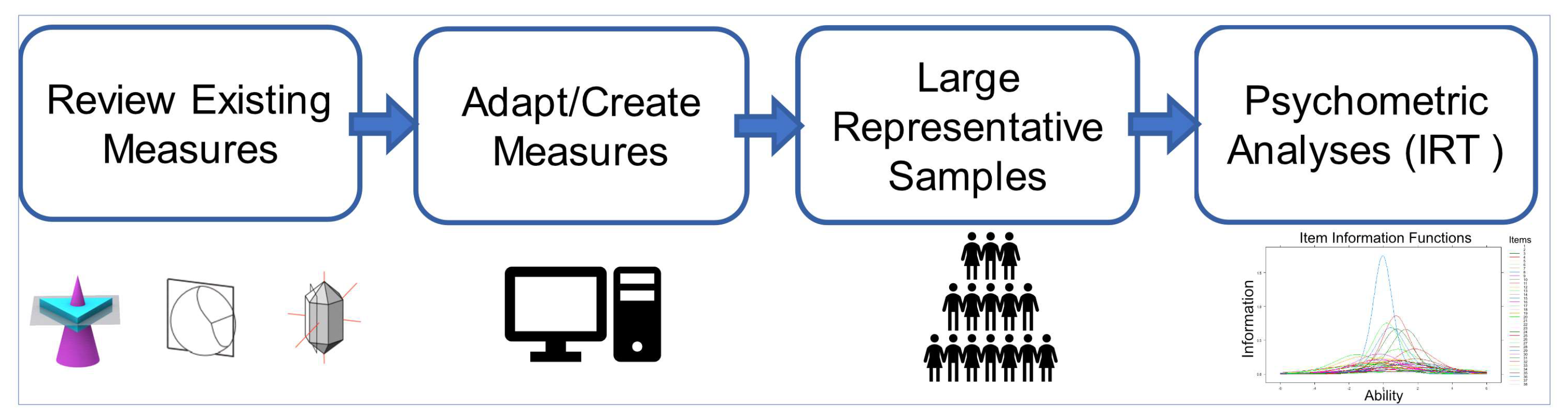
Here, we propose and demonstrate an approach to address these problems (see
Figure 1) by developing robust and efficient measures of STEM-relevant spatial abilities. The first step is to identify spatial skills that we know are related to STEM success and to review existing measures of each skill.
The second step is to adapt these measures for online testing, which, in turn, enables the collection of large samples of data representing the population at large. Most current tests exist only in paper-and-pencil forms. Because many of these tests have a time limit, individuals with lower spatial abilities typically do not complete all of the items on these tests, which has hampered the application of modern psychometric analyses, such as IRT, to these tests. Applying these techniques requires large data sets (typically of 500 or more participants), in addition to requiring responses to all test items for all participants. Adapting these tests for computer-based administration facilitates the collection of large data sets and can enable us to impose a time limit per item rather than for a whole test or subtest so that we collect data on all items from all participants.
The third step is to collect data on these tests from large samples that are representative of the general population. As noted, existing tests of spatial abilities have not been normed, or if they have, it has typically been on convenience samples of college students. Many technical careers require more practical experience or technical training rather than a college education, so it is important to examine skills across the whole adult population, and not just those who go to college. It is also important to ensure that our samples reflect the ethnic and socio-economic diversity of the population.
The fourth and final step is to subject the data to statistical analyses. First, we need to examine the internal consistency and correlations between the tests, as measures of reliability and validity. As some measures were developed for specific populations, it is also important to examine the relative difficulty of their items for the general population. Item Response Theory (IRT,
Hambleton et al. 1991) can be valuable in accomplishing these goals. IRT analysis involves fitting a model to observed responses on each item of a test based on the probability of a test taker at a given ability level getting that item correct. It offers several advantages over the classical test theory (
Hambleton and Jones 1993). First, estimated item parameters are sample independent so that the results of an IRT analysis are more accurate when generalizing to larger populations. Second, IRT provides a measure of precision, which allows the researcher to examine how precisely a test can measure the construct at different levels of ability. For example, a test item may offer a precise measure at a high level of ability but be less precise at lower ability levels. Using IRT, we can identify the most discriminating and precise items from different tests, enabling the development of efficient tests.
Our approach was informed by a recent study on the spatial perspective-taking ability.
Brucato et al. (
2022) conducted an analysis of four measures in common use to measure this ability. Correlational and IRT analyses revealed that although the four measures ostensibly measure the same ability, one test was not significantly correlated with the other three, suggesting that it measured a somewhat different ability. The other tests differed in characteristics, such as whether the display included a human figure or three-dimensional cues, but the tests measured a common ability. Item Response Theory analysis was used to identify the most discriminating items on these tests and also indicated that they differed in discriminability across the range of ability. This analysis was used to recommend a set of items that could be used to create efficient and reliable measures of perspective-taking ability. This study shows the promise of aspects of our approach but used existing paper-and-pencil measures and was limited by a relatively small sample and a college student sample. Here, we use the same approach to examine cross-sectioning tests, first adapting them for online administration. This enabled us to recruit a national sample of 18–20-year-olds, including high school students, college students, and individuals not currently in an educational institution.
1.1. Cross-Sectioning
We focus on the spatial task of inferring the cross-sections of a 3D object. While this task was not included in classic factor analyses of spatial ability measures (e.g.,
Michael et al. 1957;
McGee 1979;
Lohman 1988;
Carroll 1993), it has been identified as a spatial skill that is central to spatial thinking in science, technology, engineering, and mathematics. A cross-section is the resulting plane or flat surface after a three-dimensional object is cut using a two-dimensional plane, that is, a 2D slice of a 3D object. Cross-sections are often used in science and technology to show the internal structure of a three-dimensional object, such as a complex mechanical system or a part of the human anatomy. They are also observed in everyday activities such as cooking (slicing fruits and vegetables), and as a result, the development of cross-sectioning skills might not be dependent on formal education.
Tests of cross-sectioning have been related to achievement in biology, medicine, geology, engineering, and geometry. In biology, they are commonly used to mentally represent cross-sections of anatomical structures, and this skill is also important in interpreting medical images, such as X-rays, ultrasounds, and magnetic resonance imaging (
Hegarty et al. 2007).
Rochford (
1985) found that medical students who performed poorly on sectioning geometric solids also performed poorly (compared to high-spatial students) on practical anatomy exams.
Russell-Gebbett (
1985) found a similar pattern with younger students (age 11 to 14); specifically, students’ science ability (as rated by their teachers) correlated positively with their performance on Biology test items that required them to imagine a cross-section of a three-dimensional structure. In geology, students need to be able to visualize the internal structure of a geological formation (
Kali and Orion 1996). Engineering also draws heavily on this skill, specifically when working with blueprints and making orthographic projections (
Duesbury and O’Neil 1996;
Gerson et al. 2001;
Hsi et al. 1997). Finally,
Pittalis and Christou (
2010) identified skills such as the understanding of 2D representations of 3D objects as being a predictive factor of 3D geometric reasoning abilities. Overall, the ability to visualize cross-sections is important for success in a range of STEM fields.
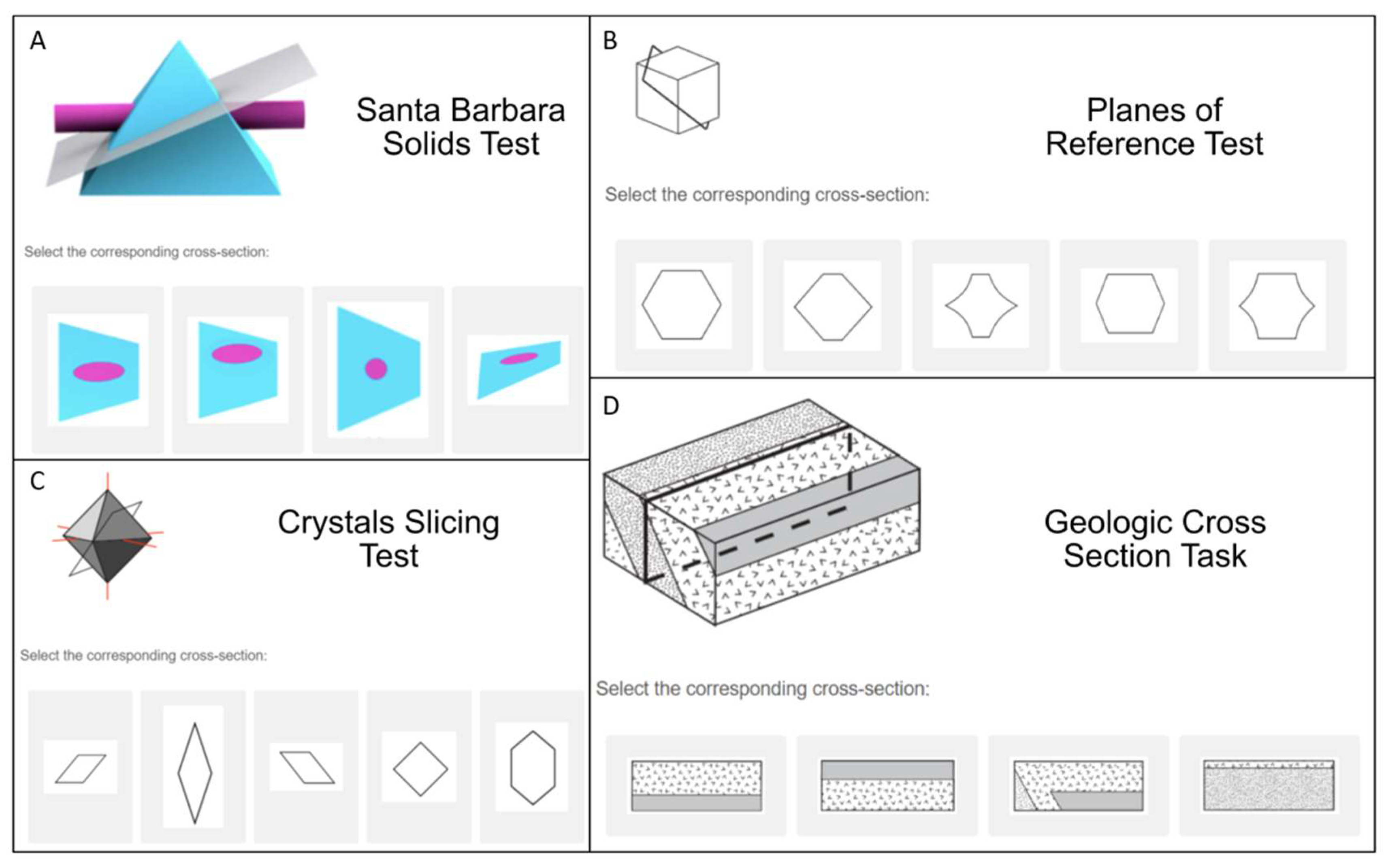
Several tests are currently in use to measure cross-sectioning ability with no agreed-upon standard. The earliest test of this ability is the Mental Cutting Test (MCT,
College Entrance Examination Board 1939), which has 25 items that show a representation of a 3D shape with a plane cutting through it and requires test takers to choose the answer that shows the shape of the cutting plane (see
Figure 2B for an example). This test is very similar to another commonly used cross-section test called the Planes of Reference test (PRT,
Titus and Horsman 2009), a 15-item test with the same instructions as the MCT but with distinct items. In both of these, the figures are shown as line drawings with limited depth cues. Another test, also referred to as the Mental Cutting Test or “Schnitte” (
Quaiser-Pohl 2003), shows similar figures to the MCT but uses a different method of responding (“select all that apply” rather than choosing one correct answer out of five choices). These tests likely involve similar spatial visualization processes but afford different analytic strategies due to the response formats.
Cohen and Hegarty (
2007) developed the Santa Barbara Solids Test (SBST), with the same multiple-choice format as the original Mental Cutting Test and Planes of Reference test but different stimuli that were rendered with 3D imaging software and included shading to provide depth cues (see
Figure 2A). The items were designed to vary in difficulty based on two aspects: the geometric complexity of the solid and the orientation of the cutting plane. Finally, a number of tests of cross-sectioning ability were designed for studies of specific STEM disciplines. Some examples include the Crystal Slicing Test (CST,
Ormand et al. 2017), the Geologic Block Cross-Sectioning test (GBCST,
Ormand et al. 2014) designed for testing Geology students, and the tooth cross-section test (
Hegarty et al. 2009) designed for testing dental students. The Crystal Slicing Test (see
Figure 2C) shows 3D crystals found in mineralogy, while the Geologic Block Cross-Sectioning Test (See
Figure 2D) shows sections via geological structures. The tooth cross-section task uses 3D figures of a tooth with roots inside and, like the Geologic Block Cross-Sectioning test, involves visualizing internal structure, so these tests are often referred to as tests of penetrative thinking (
Kali and Orion 1996).
1.2. This Present Study
This present study began by comparing performance on four of the existing cross-section tests: the Santa Barbara Solids Test (
Cohen and Hegarty 2007), the Planes of Reference Test (
Titus and Horsman 2009), the Crystal Slicing Test (
Ormand et al. 2017), and the Geologic Block Cross-Sectioning test (
Ormand et al. 2014; see examples of test items in
Figure 1)
1. First, these tests were adapted for online administration via Qualtrics. After piloting the online tests with a college sample, we removed the Geologic Block Cross-Sectioning test from further analysis due to its difficulty and time constraints and administered the remaining three tests in an online study. This enabled us to collect a large data set necessary to conduct Item Response Theory analyses from a sample that is more representative of the US population.
One goal of the research was to examine the psychometric properties of existing tests. We first examined the internal consistency of these tests and their inter-correlations to assess their reliability and validity and whether they measure a common ability despite the differences between the tests (e.g., 3D depth cues, type of structure to be sectioned, etc.). Next, we applied IRT analysis to establish whether items on each test measure a common ability or capture unique variance and to assess the difficulty and discriminability of the items on each test. This enabled us to construct an efficient measure of cross-sectioning, made up of the most discriminating items on the existing tests, a second goal of this research.
Using this refined test, we then considered different models of the cognitive processes underlying the cross-sectioning ability by examining possible subcomponents of this ability and aspects of items that affect their relative difficulty. First, we considered the orientation of the cutting plane. Previous research with the Santa Barbara Solids Test indicated that people scored lower on items with cutting planes that are oblique to the reference frame of the object than for orthogonal cutting planes (
Cohen and Hegarty 2007,
2012), possibly because people have more experience with near-orthogonal cuts in everyday life (e.g., when slicing vegetables). Although it is unlikely that these everyday cross-sections are perfectly orthogonal, they are generally close to shapes created by an exact 90° cut. Oblique cuts might also be more difficult to identify correctly because of a tendency to infer that a 2D shape would extend orthogonally into 3D space, not obliquely, and so we might tend to visualize a rectangle as an orthogonal cut of a rectangular prism instead of an oblique cut of a cube (
Gagnier and Shipley 2016). Similarly, using the Mental Cutting Test,
Tsutsumi (
2004, p. 117) identified two types of items: “pattern” problems, which only require recognizing the shape of the cut to solve it (e.g., a rectangle), and “quantity” problems, which also require identifying metric properties of the shape (e.g., the aspect ratio of the correct shape). Second, we considered the complexity of the solid, including the number of parts making up the solid, which has also been found to affect difficulty (
Cohen and Hegarty 2007,
2012). Therefore, we also considered models that took complexity into account.
Finally, we examined how demographic variables (including sex, age, ethnicity, and mathematics education) are related to cross-sectioning performance. Sex differences are found in some but not all spatial ability measures (
Linn and Petersen 1985;
Voyer et al. 1995), so it is important to establish whether these differences exist (and the size of any differences) for different spatial measures. To our knowledge, this is the first study to examine sex differences in cross-section tests with a large sample. In contrast to sex differences, there has been relatively little research on the relationship between ethnicity and spatial performance. Here, we compared the performance of Hispanic and non-Hispanic participants. Because cross-sections are studied to some extent in geometry and cross-section diagrams are prevalent in scientific textbooks, it is also possible that this spatial skill is affected by education, so we compared the performance of individuals with different levels of education (e.g., high school vs. college) and explored the effects of parental education and taking math courses.
1.3. Study 1: Pilot with University Students
A pilot study was conducted with university students to assess the feasibility of administering cross-section tests online, to measure the average time taken to respond to items in the cross-section tests, and to establish basic levels of performance for a general college population on the four tests.
3. Results
Descriptive statistics and measures of reliability for the four tests are presented in
Table 1. McDonald’s Omega measures general factor saturation. Internal consistency was calculated using Spearman–Brown (
Spearman 1904) corrected split-half reliability using the ‘splithalf’ package in R (
Parsons et al. 2019) and Cronbach’s Alpha. Mean performance on the Santa Barbara Solids Test was well above chance (95% CI [17.26, 21.39], chance = 7.5), and this test also showed good reliability. The performance of the Planes of Reference (95% CI [6.38, 8.23], chance = 3) and Crystal Slicing (95% CI [7.39, 9.12], chance = 3) tests were also well above chance, but these tests showed only moderate reliability. The mean performance of the Geologic Block Cross-Sectioning Test was significantly above but close to chance (95% CI [4.87, 6.66], chance = 4), and this test also showed moderate reliability.
Response times per item were similar for the SBST, PRT, and CST (see
Table 1). The median response times for these tests were 10.46, 10.78, and 11.43, respectively, and only five participants had median response times of more than 20 s per item on any of these tests. In contrast, the mean (see
Table 1) and median (16.88) response times for the GBCST were substantially longer, and 31.1% of response times were more than 20 s. As shown in
Table 2, correlations between the tests were high, especially after correcting for the reliability of the measures, suggesting that they share considerable variance.
6. Results
6.1. Scoring
Correct answers were coded as 1, and incorrect answers were coded as 0. If a participant reached the time limit of 20 s for a problem without selecting an answer choice, they were assigned a score of 0 for that problem. The time limit was reached with no answer selected on a mean of 3.2% of items.
6.2. Descriptive Statistics
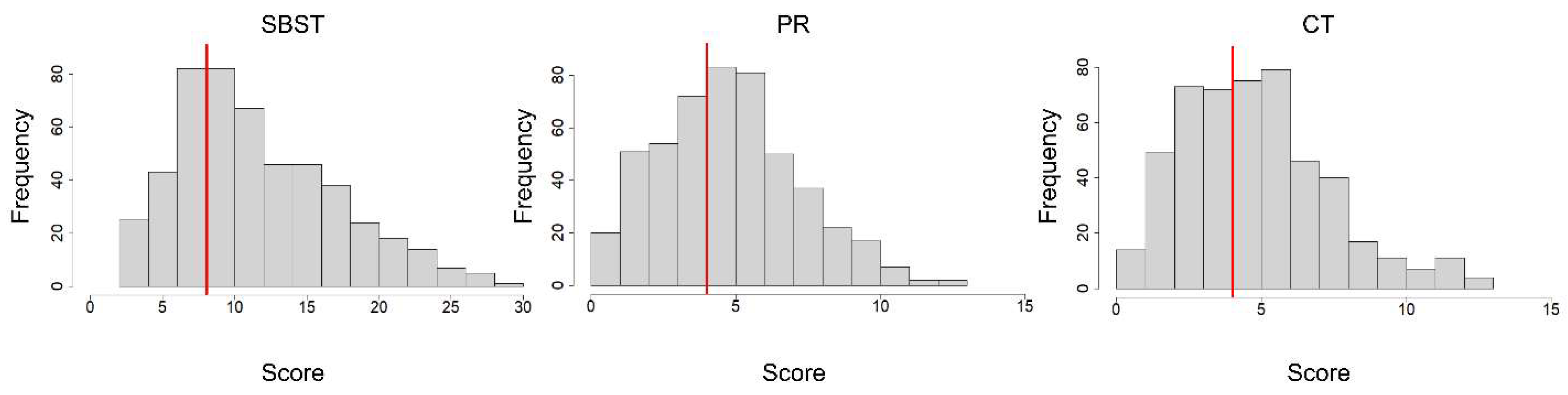
Descriptive statistics for the measures are shown in
Table 4, and histograms showing their distributions are in
Figure 4. The average scores on the three cross-section tests were above chance levels (chance was 7.5 for the SBST and 3.0 for both the PRT and CST). However, they were closer to chance than for the college student sample in Study 1. The average scores were 12.10 on the SBST, 5.24 on the PRT, and 5.28 on the CST. The average response times for the cross-section tests (see
Table 4) were well within the imposed time limit of 20 s. The performance of the Word Sum test was also above the chance level (2.8) and was not timed in this administration.
6.3. Reliability and Correlations
Internal consistency and general factor saturation (McDonald’s Omega) for the four measures are shown in
Table 4. Internal consistency was calculated using Spearman–Brown (
Spearman 1904) corrected split-half reliability using the ‘splithalf’ package in R (
Parsons et al. 2019) and Cronbach’s Alpha. Like in Study 1, the Santa Barbara Solids Test showed good reliability, while the reliability of the Planes of Reference and Crystal Slicing Tests was moderate. As shown in
Table 5, correlations between the tests were moderate and remained significant after controlling for verbal ability (Word Sum test), indicating that, as expected, the cross-section tests shared common variance related to spatial processing and not just motivation or general intelligence (providing evidence for divergent validity). The disattenuated correlations between the measures were also calculated, taking their reliabilities (i.e., permutation-based split-half estimation) into account (
Parsons et al. 2019). The disattenuated correlations between the cross-section measures were high (0.90 or greater), indicating considerable common variance. Disattenuated correlations are reported above the diagonal in
Table 5.
6.4. Unidimensionality and Local Independence
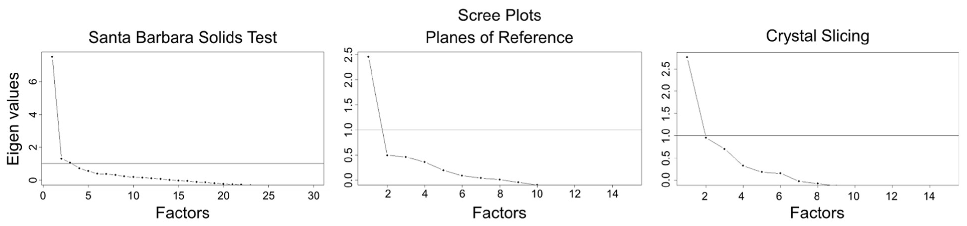
We conducted an exploratory factor analysis from the tetrachoric correlation matrices to assess whether each of the cross-section tests measured a unidimensional ability, using two criteria to assess the number of factors (dimensions) underlying performance, the number of factors with Eigenvalues greater than 1, and the Scree test (
Cattell 1966). The first factor in the SBST had an Eigenvalue of 7.52, while the second and third Eigenvalues were just over 1 (1.29 and 1.05, respectively). The first factor was clearly dominant, and the scree plot suggested one factor (see
Figure 5). The PRT also showed a dominant first factor (first Eigenvalue = 2.45, second Eigenvalue = 0.49), as did the CST (first Eigenvalue = 2.76, second Eigenvalue = 0.95), and for these tests, only Eigenvalues of the first factor exceeded 1, again suggesting unidimensionality.
The tests were also assessed for local independence of items. If a person’s score on one item predicts their score on another item after accounting for the main factor of cross-section ability, the pair of items is said to be locally dependent and likely share a common feature separate from cross-sectioning. To test for local dependence, the G
2 statistic (
Chen and Thissen 1997) and the Jackknife Slope Index (JSI;
Edwards et al. 2018) were calculated for each possible combination of items in each individual test using the
residuals function in the R package
mirt (
Chalmers 2012). In order to examine each model for possible locally dependent item pairs, the distribution of the standardized values of G
2 and JSI for all item pairs was inspected (see the range for each diagnostic in
Table 6). There was no evidence of local dependent item pairs.
6.5. Within Task Item Response Theory Analyses
We tested the fit of the data for each test to the single-factor, two-parameter logistic model (2PL), which includes estimated parameters for discriminability and difficulty for the test items. All models were fit using the “mirt” package in R (
Chalmers 2012) using the Expectation Maximization (EM) algorithm (
Bock and Aitkin 1981).
Table 7 presents the model fit for each test. The overall model fit for each test was assessed using the M
2 statistic, which has been demonstrated to be less influenced by the sparsity of the contingency table of response patterns than chi-square (
Maydeu-Olivares 2014), as well as Root Mean Square Error of Approximation (RMSEA), Comparative Fit Index (CFI), Tucker–Lewis Index (TLI), and Standardized Root Mean Squared Residual (SRMR). Acceptable fit was determined based on the following criteria: Root Mean Square Error of Approximation (RMSEA) below 0.05 (
Maydeu-Olivares 2013), Comparative Fit Index (CFI) above 0.95, Tucker–Lewis Index (TLI) above 0.95
3, and SRMR less than 0.05 (
Maydeu-Olivares 2013). While a significant M
2 indicates that we should reject the null hypothesis of the fitted model being true, this statistic was small relative to the degrees of freedom (
< 3), indicating an acceptable model fit.
6.6. Santa Barbara Solids Test
For the SBST, the unidimensional 2PL model is not a good fit based on all model fit diagnostics, but most were close to the cutoffs. The individual items of SBST were also examined to check for sources of model misfit. A well-fitting item will have a non-significant p-value in a test of chi-square, indicating that the model’s generated data were not significantly different from the observed data. Item 8 showed marginally significant misfit (p = .025). However, the RMSEA of this item is 0.038, which is still well within the acceptable range (<0.05). Removing item 8 and re-running the model results in another item being significantly misfit, and this repeats if the next item is also removed. As such, the overall model fit does not improve by removing item 8, and it was maintained.
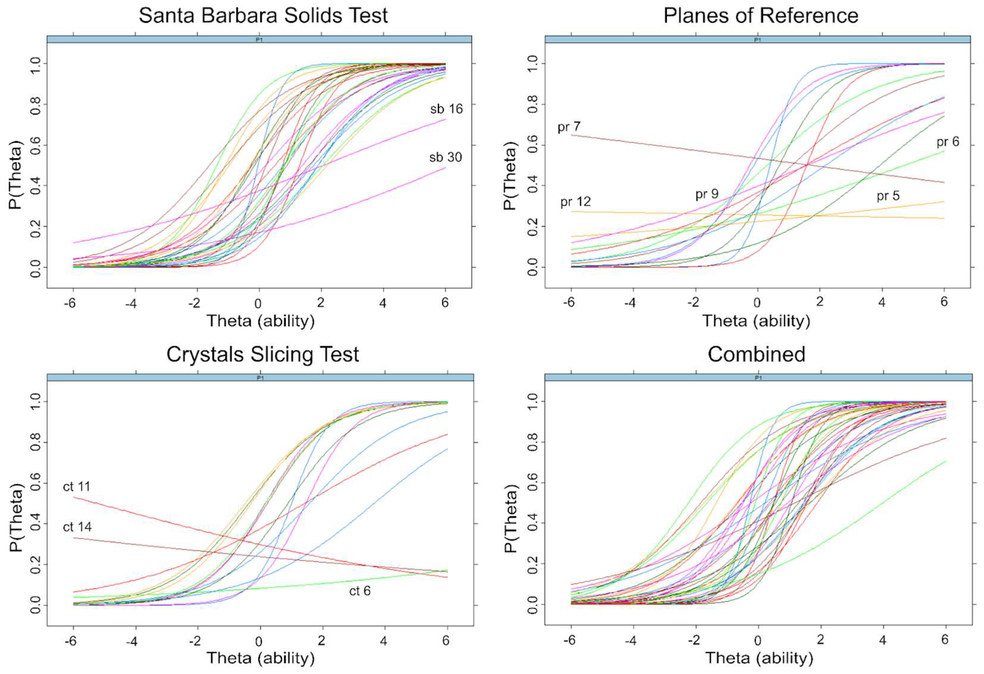
Item characteristic curves (ICC) shown in
Figure 6 visualize the estimated parameters of discriminability and difficulty for each item of the tests (See
Supplementary Table S1 for all SBST item parameters). The slope of each ICC represents the discriminability of one item. If an ICC for a given item is flat (i.e., has a low slope), this indicates low discriminability such that at low levels of ability (x-axis), the probability of getting the item correct (y-axis) is not much lower than at high levels of ability. The location of an ICC on the x-axis indicates its difficulty, with items to the right indicating more difficulty.
The mean discriminability coefficient for all 30 SBST items was 0.98 (moderate), and they ranged from 0.25 (very low) to 2.58 (very high). As seen in
Figure 4, items 16 and 30 do not discriminate well between high and low levels of ability. The discriminability coefficients of these items were less than or equal to 0.26. In both of these items, there were two answer choices that were very similar. These items were removed to improve the efficiency of the test. The mean discriminability coefficient for the remaining 28 items was 1.04 and ranged from 0.67 to 2.59.
The mean of the difficulty coefficients for the SBST was −0.49, meaning the items were somewhat difficult (a test-taker with average ability would have a less than 50% chance of getting an item correct on average). The item difficulties ranged from −2.12 (very difficult) to 1.73 (very easy). After removing items 16 and 30, the average difficulty coefficient was −0.46, and the range did not change.
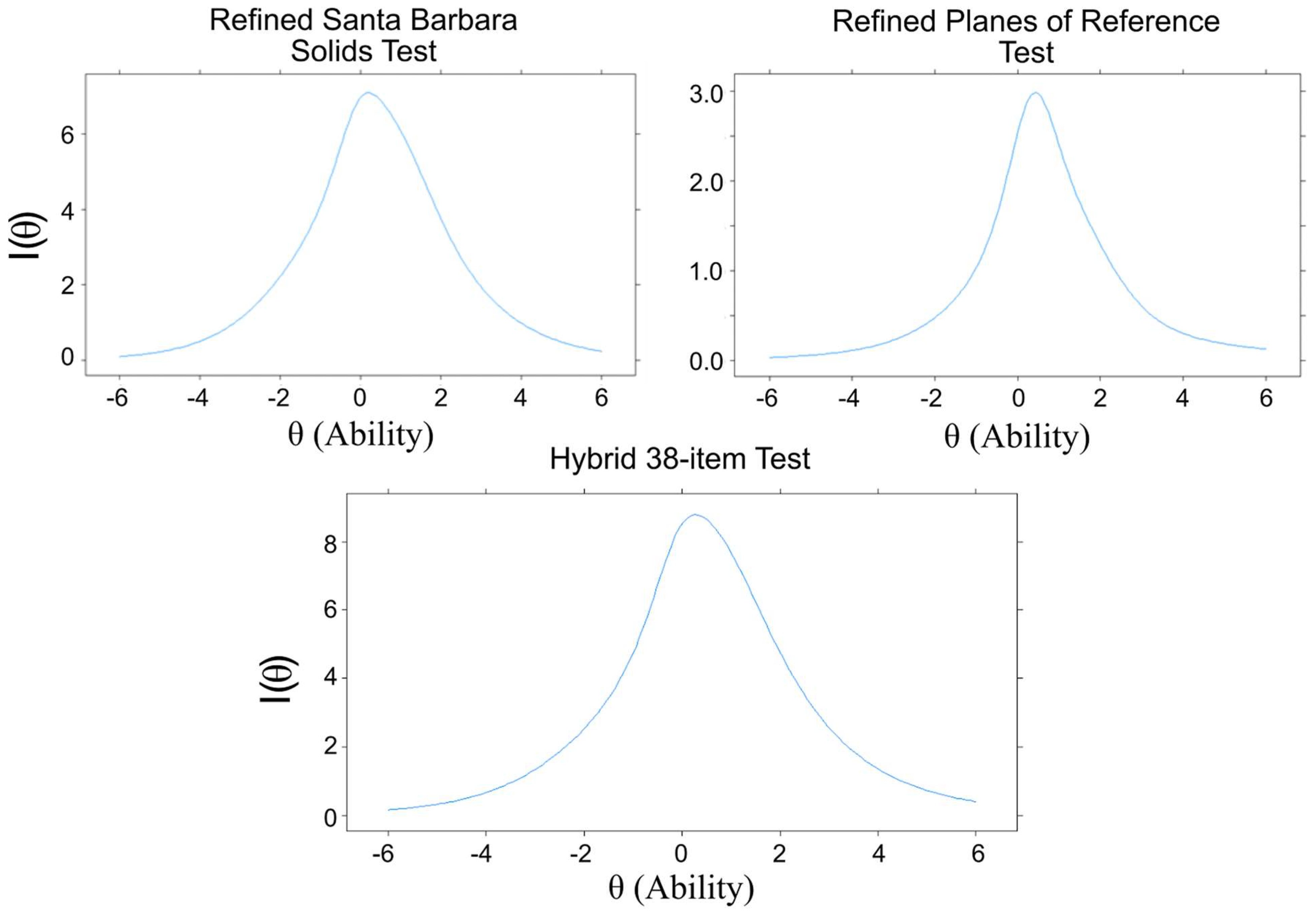
The Test Information Function (TIF,
Figure 7) shows how much information the overall tests capture at a given level of ability. For SBST, the curve of the TIF was highest around average to slightly above-average ability (theta = 0 to 0.5), meaning the test is more precise when measuring test takers in this ability range. Overall, the test should perform well on test takers between moderately low (theta = −1) and high (theta = 1.5) ability levels, with the most precision around average (theta = 0) ability.
6.7. Planes of Reference Test
For the Planes of Reference Test, the unidimensional 2PL model fits acceptably by all criteria (see
Table 7). The fit of individual items was assessed using a signed chi-square, and there were two marginally misfit items (item 2,
p = 0.022, and item 9,
p = 0.039). As with the SBST, these items had acceptable RMSEAs at 0.05 or less. The model fit did not improve with the removal of these items, and they were maintained in the refined version of the test.
The average discriminability for all PRT items was 0.68, and it ranged from −0.08 (very low) to 2.45 (very high). The average difficulty was −0.78 (moderately difficult) and ranged from −2.45 (very difficult) to 0.29 (average). All items with a discriminability coefficient less than 0.26 (items 5, 6, 7, 9, and 12) were removed in order to improve test efficiency, leaving 10 items. The discriminability coefficients of these 10 items ranged from 0.35 to 2.45. The TIF of the overall PRT test (
Figure 4) shows the most precision for test takers of average to above-average ability (thetas from 0 to 1). See
Supplementary Table S2 for all PRT item parameters.
6.8. Crystal Slicing
Overall, the Crystal Slicing Test did not show an acceptable model fit. The RMSEA of the model was acceptable, but the CFI, TLI, and M
2 significance tests indicated a poor fit (see
Table 7). The consideration of individual items indicated that items 2, 10, and 14 showed significant misfits (
p < .05). Item 10 had the highest RMSEA (0.081), while the other two were within acceptable bounds (≤0.05). While there were not any obvious problems with these items upon inspection, one possible source of error for non-geology students might have misinterpreted the symmetry of the shapes as they are unlikely to be familiar with these shapes.
After removing items 2, 10, and 14 and fitting a new 2PL model, the model fit improved but still did not fit acceptably (p < .001, RMSEA = 0.049, CFI 0.85, TLI 0.82). The removal of three more items (1, 6, 9) that have significant misfits in the new model (p < .05) indicated a poorer fit of the overall model. The remaining nine items did not show any individual misfits. Thus, removing any more items would not improve fit. In sum, the 2PL model does not fit the observed data for the Crystal Slicing Test, and as a result, it was not included in the analysis of the combined tests.
6.9. Combined Task Item Response Theory Analysis: Model Comparisons
A refined 38-item cross-section test was created comprising the 28 SBST and 10 PRT items that showed good discriminability. The SBST images of the solids to be sliced had depth cues, including shading, while the PRT items showed line drawings with limited depth cues (see
Figure 2) and, therefore, may have depended more on familiarity with graphical conventions (
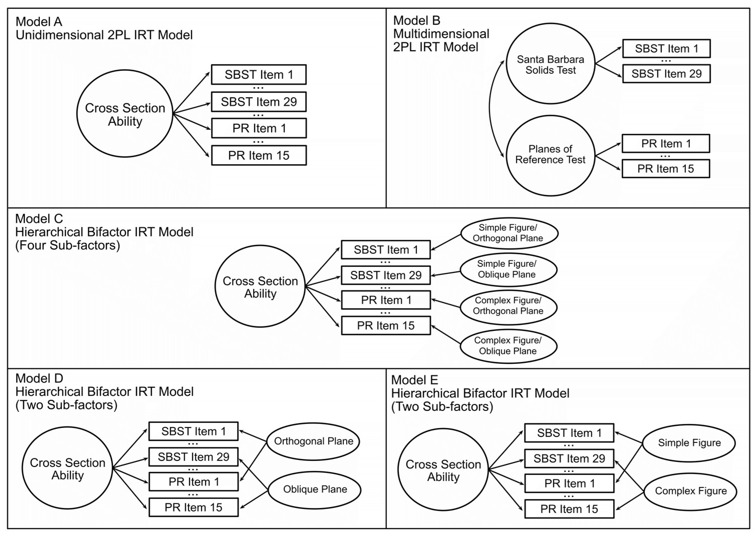
Bartlett and Camba 2023b). To examine whether the items from these two tests measured distinct abilities, we compared a unidimensional 2PL model (Model A,
Figure 3), indicating that all 38 items measure a common dimension of ability, to a non-hierarchical multidimensional 2PL model (Model B,
Figure 3), indicating that the two tests measure distinct but correlated constructs. In the non-hierarchical multidimensional (two-factor) 2PL model (Model B) items from the SBST were constrained to load on one factor, and items from the PRT were constrained to load on a second factor. The unidimensional 2PL model (Model A) showed an acceptable fit to the observed responses (see
Table 8). The overall fit of the two-factor model (Model B) was poorer than for Model A (see
Table 8), supporting the idea that the tests were measuring the same, rather than distinct abilities, despite the differences in depth cues provided. In the unidimensional model, all items showed a good fit (
p > .06). The least discriminable items were PRT 11 (discriminability = 0.298) and PRT 10 (discriminability = 0.410). Items functioned well over a wide range of abilities (thetas = −2 to 2). The overall test captured the most information around average to just above average ability but also captured a good amount from moderately low ability (theta = −1) to high ability (theta = 2) levels (see
Figure 5). This test showed high factor saturation (McDonald’s Omega = 0.86) and high reliability (split-half reliability = 0.83; Cronbach’s Alpha = 0.85).
Previous research indicated that both the orientation of the cutting plane and the complexity of the solid to be sliced affect the difficulty of items on the SBST (
Cohen and Hegarty 2007). To examine whether these item characteristics defined sub-factors, we evaluated a hierarchical bifactor model (Model C, see
Figure 2). Sometimes referred to as a two-tier model, ‘bifactor’ refers to the general factor
g that all items are assumed to load on (i.e., the second tier) and the first tier, which can contain any number of sub-factors, up to the number of items on the test (
Gibbons and Hedeker 1992;
Chalmers 2012). Model C assumed each item to load on a general factor (cross-section ability) but was also constrained to load on one of four sub-factors, identified based on
Cohen and Hegarty’s (
2007) classification. Figures were classified as either
simple or
complex, and the orientation of the intersecting plane was classified as either
orthogonal or
oblique (relative to the x, y, or z-axis of the figure), resulting in four possible sub-factors (7
simple orthogonal;
11 complex orthogonal;
8 simple oblique; and
12 complex oblique). The bifactor model showed a very good fit to the observed data (see
Table 8), with a better fit than Model A or B, indicating that the 38-item hybrid test is measuring one general factor of cross-section ability, but responses are also influenced by sub-factors of each item.
Finally, we considered more parsimonious bifactor models that specified only the orientation of the intersecting plane (Model D) and only the complexity of the figure (Model E) as sub-factors. As shown in
Table 8, Model D fit the observed data significantly better than Model C (AIC and BIC decreased by 80.37, chi-square = 80.37,
p < .001). In contrast, Model E was a poorer fit than Model C (AIC and BIC increased by 25.28, chi-square = 25.28,
p < .001) and Model D (
p < .001, Vuong’s test of non-nested models). Model D fits significantly better than Model A,
p < .001, using Vuong’s test of non-nested models. These analyses and the principle of parsimony indicate that the best-fitting model was one with a general factor for cross-sectioning reflecting items from both the SBST and the PR, with sub-factors for items with oblique and orthogonal cutting planes. See
Supplementary Table S3 for all Model D item parameters
4.
6.10. Individual Differences
The 38-item refined test was used to examine the effect of demographic variables on cross-sectioning ability (see
Figure 7). We examined this using both the summed score of the 38 items and Theta estimates (ability scores) from Model D. As shown in
Table 9, correlations with the demographic variables were almost identical for the two measures, so we used summed scores for these analyses (the significance of the correlations with sex were marginal, reaching significance in one case). There was no significant sex difference in the score (males’ mean score = 15.73,
SD = 7.14, females’ mean score = 14.53,
SD = 6.47;
p = .05, Cohen’s
d = 0.18). There was no significant ethnicity difference (Hispanics’ mean score = 14.96, non-Hispanics’ mean score = 15.17;
p = .76). A one-way ANOVA tested for differences between educational status groups (in high school, graduated from high school, in college), but no difference was found (
F (1,496) = 0.31,
p = .58). Participants whose parents’ education was higher (college degree or above) had significantly higher scores (
M = 16.52,
SD = 7.31) than those whose parents’ education was lower (
M = 14.17,
SD = 6.31;
p < .001,
d = 0.35), and there was a significant, positive correlation between score and reported number of math courses taken (
r = 0.24,
p < .001) and Word Sum score (
r = 0.39,
p < .001). Age (18–20) was not significantly correlated with score but was correlated with educational level (
r = 0.11,
p < 0.01), probably because older participants were more likely to have more education.
As the demographic variables were somewhat correlated (see
Table 9), we conducted a regression analysis with performance (total score) as the outcome variable and the following predictors: sex (male = 0, female = 1), age (18–20), number of math courses taken (1–10), parents’ education (1–5, 1 = did not finish high school, 5 = graduate or professional degree), current education status (1–3, 1 = in high school, 2 = graduated from high school, 3 = in college), and verbal ability (Word Sum score). All predictors except sex were standardized. The results of the regression model using summed scores as the measure of ability are shown in
Table 10 (results of the model using theta as the ability measure are in
supplementary materials). When accounting for all demographic variables, only the number of math courses and Word Sum score significantly explain variance in performance. The total variance explained using the model is R
2 = 0.19,
F(6, 491) = 18.79,
p < 0.01.
6.11. Creating A Refined, Efficient Test
In order to create an efficient test of cross-section ability, 20 items were selected from the combined 38-item based on item discrimination and difficulty coefficients in Model D. Of the 20 items, 15 were from SBST, and 5 were from PRT, with 14 orthogonal-plane items and 6 obliques. Since test information on the 38-item test was more precise for higher-ability than lower-ability participants, items with the lowest discrimination (range: 0.392–0.909) that also had average to high difficulty (range: −1.748 to 0.190) were removed. There were four items that had lower discriminability (range: 0.630–0.807) but were not removed in order to balance the number of lower difficulty items (range: 0.325–1.305). The average discriminability of the items in the 20-item test was 1.39 (moderately high), and the average difficulty was 0.04 (average). The range of discriminability of the 20 items was 0.538 (low) to 2.802 (very high), and the difficulty ranged from −2.183 (very difficult) to 3.110 (very easy). The internal reliability of the 20 items was high (split-half reliability = 0.78, McDonald’s Omega = 0.84). The Bifactor model with just the refined 20 items using two factors (orthogonal plane or oblique plane, referred to as model 20-D in the table) showed a very good fit to the observed data (see
Table 8).
7. Discussion
The goals of this study were to evaluate current tests of crossing section ability using modern psychometric techniques, create an efficient test of this ability that is usable across the ability range of the general population, examine possible subcomponents of this ability, and conduct preliminary analyses of how it is related to demographic variables, including sex, ethnicity, and education.
First, in order to collect data from a large sample, several commonly used paper-and-pencil tests of cross-section ability were adapted for online administration. This involved adapting the tests so that one item was shown at a time and time limits were per item (based on piloting in Study 1) rather than for the whole test. This also ensured that we collected data on all (or most) items from all participants, as is necessary for Item Response Theory analyses. Online administration (via Qualtrics Panels) also allowed us to collect a sample that is more representative of the broader population than typical convenience samples of college students. Participants were 18-to−20-year-olds, recruited to match the demographics of Naval recruits, and included participants still in high school, enrolled in college, and graduated from high school without being enrolled in further education. This enabled us to develop a test that can be used to identify individuals who have the potential to excel in both technical careers and STEM education.
One goal of our analyses was to provide information on the psychometric properties of existing tests. Our analyses indicated that while the tests were correlated, the Santa Barbara Solids Test (SBST) and the Planes of Reference Test (PRT) had good psychometric properties, while the Crystal Slicing Test (CST) did not. Moreover, the CST test was difficult, and another test, the Geological Block Cross-Section Test (GBCST), was eliminated from consideration after Study 1 as it was deemed too difficult for college students. Both the CST and the GBST were developed for studies involving Geology students (
Ormand et al. 2014,
2017), so it is likely that they measure geology knowledge in addition to cross-sectioning ability (analogous to other domain-specific tests such as the Tooth Cross-Section test,
Hegarty et al. 2009). However, their correlations with the SBST and PRT indicate that they also measure a more general ability to imagine cross-sections of three-dimensional structures in addition to domain knowledge. The domain-general cross-section test developed here can be used to identify students who are likely to benefit from specific training on cross-sectioning before taking advanced classes in STEM-related disciplines such as geology and anatomy that depend on this skill. More domain-specific cross-section tests might then be used to evaluate their performance in the relevant classes.
The Planes of Reference and Santa Barbara Solids Tests differed in the provision of depth cues to depict the structure of three-dimensional solids in the two dimensions of the printed page. Our analyses indicated that they appeared to measure the same construct, such that a model indicating a single ability underlying these two tests (Model A) was a better fit to the data than a model (Model B), assuming that they measured distinct abilities. Although it has recently been argued that the interpretation of impoverished graphics (with limited depth cues) may be a source of difficulty in spatial ability measures (
Bartlett and Camba 2023b), it appears that the difference in depth cues provided by these two tests is not a major source of variance. That is, although these two tests differ in the depth cues provided, they measure a common ability.
Cohen and Hegarty (
2007) proposed two characteristics of cross-section items that might affect their difficulty: the orientation of the cutting plane and the complexity of the figure. But, they found that only the orientation of the cutting plane had an effect. Here, we examined whether these characteristics defined different sub-factors of the cross-sectioning ability and found that the data were best fit by a hierarchical model (Model D) that assumes a general factor and sub-factors reflecting the orientation of the cutting plane (orthogonal or oblique). Consistent with previous research (
Cohen and Hegarty 2007) participants made fewer errors on items on orthogonal sections (mean correct = 0.46,
SD = 0.20) than oblique (mean correct = 0.32,
SD = 0.19;
t = 19.37,
p < 0.001). We speculate that these items were easier because people have more experience viewing near-orthogonal cross-sections in everyday life (e.g., when slicing vegetables) because they tend to assume that a 2D shape extends orthogonally into 3D space, even for oblique sections (
Gagnier and Shipley 2016) or because orthogonal sections often require just recognizing the shape of the resulting cross-section (e.g., a square) rather than identifying metric properties of a shape (e.g., a more or less eccentric rectangle), as suggested by
Tsutsumi (
2004). Interventions to train cross-sectioning ability might use orthogonal cross-sections to scaffold the ability to imagine more difficult oblique cross-sections.
Sex differences are found in some spatial tests (e.g., mental rotation) but not others (
Linn and Petersen 1985;
Voyer et al. 1995). Because mental rotation is the most commonly used measure of spatial ability (
Hegarty 2018;
Bartlett and Camba 2023a), this may overemphasize the existence and size of sex differences in spatial ability, and it is important to document the size of any sex differences when validating measures. Although close to significance, there was no sex difference in ability found in this study, and the effect size was small (
d = 0.18) compared to the effects commonly found in tests of mental rotation (
d = 0.67,
Voyer et al. 1995). More generally, a moderate effect of parental education level (
d = 0.35) and a small correlation (
r = 0.24) with the number of math courses taken suggest that cross-section ability is somewhat influenced by educational opportunities and other socioeconomic-related experiences. In contrast, ethnicity and current educational status (high school, graduated from high school, or in college) had no effects on performance. When all demographic variables were entered in the same linear model, only math courses and verbal ability predicted performance in the refined measure of cross-sectioning. Importantly, there was no significant effect of sex in this model, indicating no appreciable sex differences in this spatial thinking task.
We set out to create an efficient cross-section measure that provides accurate and precise measurement across a wide range of abilities. Using the discriminability and difficulty estimates of each item in the best-fitting IRT model (see Model D above), we eliminated items that contributed less information, resulting in a 20-item hybrid test containing items from Santa Barbara Solids and Planes of Reference. Based on the response times in this study, participants should be able to complete the shortened test in under 10 min, including instructions. The test was most accurate for assessing participants close to average ability and within two standard deviations above or below average. As such, this test should be useful for assessing the cross-section ability of most of the population.
Limitations and Future Directions
Online data collection presents a series of challenges for maintaining a high level of data quality. Several steps were taken to ensure that participants were making a good effort on the tests; however, as they were administered online, there is no way to know if less well-performing participants understood the instructions or made their best effort. With paid survey-takers, there was concern that some participants would quickly skip through the tests, indicating a lack of effort. It is a known problem that online panels include “superworkers” who make up a very small percentage of all workers but complete a large percentage of available tasks (
Robinson et al. 2019), and Qualtrics Panels does not make it possible to select only naïve participants. We identified a subset of participants who responded very quickly on most tests and had close-to-chance performance, but rerunning the analyses without these participants did not change the models appreciably. These issues might be mitigated in future studies by including more manipulation checks to detect unmotivated participants, by giving participants feedback on their performance, which may motivate them to try their best (
Condon and Revelle 2014), or by gamifying the tests (
Malanchini et al. 2020). Time limits were determined using pilot data. However, response times were not analyzed for each item. Likely, more difficult items would require more time, and an item-level analysis of response times could serve to further refine these tests, but that is beyond the scope of this study. In future research, it will also be important to validate this measure against success in both technical occupations and STEM disciplines.


