Article

Effects of Fractional Derivatives with Different Orders in SIS Epidemic Models

1
Istituto per le Applicazioni del Calcolo, Consiglio Nazionale delle Ricerche, 00185 Rome, Italy
2
Dipartimento di Scienze di Base e Applicate per l’Ingegneria, Sapienza Università di Roma, 00161 Rome, Italy
*
Author to whom correspondence should be addressed.
These authors contributed equally to this work.
Computation 2021, 9(8), 89; https://doi.org/10.3390/computation9080089
Submission received: 15 July 2021 / Revised: 3 August 2021 / Accepted: 4 August 2021 / Published: 8 August 2021
(This article belongs to the Section Computational Biology)

Abstract

:
We study epidemic Susceptible–Infected–Susceptible (SIS) models in the fractional setting. The novelty is to consider models in which the susceptible and infected populations evolve according to different fractional orders. We study a model based on the Caputo derivative, for which we establish existence results of the solutions. Furthermore, we investigate a model based on the Caputo–Fabrizio operator, for which we provide existence of solutions and a study of the equilibria. Both models can be framed in the context of SIS models with time-varying total population, in which the competition between birth and death rates is macroscopically described by the fractional orders of the derivatives. Numerical simulations for both models and a direct numerical comparison are also provided.

1. Introduction

The interest of the scientific community in mathematical modeling for epidemiology has grown considerably in recent years. The study of epidemic models began in the early 1900s with the pioneering work of Kermack and McKendrick [1]. Their idea was to divide the population into groups that distinguish individuals based on their status with respect to the infection, giving rise to the compartmental modeling for epidemics. The evolution in time of the disease is then described by a system of ordinary differential equations for each considered class.
In this work we focus on the SIS (Susceptible–Infected–Susceptible) model [2], describing infections that do not confer immunity to recovery from illnesses such as influenza and common cold. This theory describes compartmental models, where the population is divided into groups depending on the state of individuals, that is, with respect to disease, distinguishing between infected and susceptible. The use of mathematical models for epidemiology is useful to predict the behavior of an infection and make strategic decisions in emergency situations to limit the spread of the disease, which is microscopically modeled by the fractional order of the derivative. In recent years, the use of fractional derivatives for epidemic models has grown widely. The main advantage of fractional calculus is that it can incorporate memory effects into the model. Moreover, fractional models have an extra degree of freedom compared to classical models, which is particularly useful for fitting real data when available. We refer to [3] for a recent review of fractional epidemic models.
In this paper, we consider two fractional SIS models. One model is based on the Caputo derivative, for which we establish the existence of results of the solutions and provide numerical simulations. The novelty is to allow the susceptible and infected population to evolve according to different fractional orders: the mathematical setting, in which this type of models has to be considered, needs to be deeply investigated in order to select problems that enjoy existence, uniqueness and closed-form solutions. We refer to [4] for a stability analysis of a Lotka–Volterra predator-prey fractional model with Caputo derivative and different orders of derivative, and to [5] for the case with the same order of derivative. in the framework of epidemic models, we refer to the paper [6], in which an HIV model is analyzed with different orders of fractional derivatives in the Caputo sense.
The other model is based on the Caputo–Fabrizio operator. Here we let the susceptible population evolve according to the Caputo–Fabrizio fractional operator, whereas the infected population dynamics are based on an ordinary differential equation. in this case, we rewrite the system as a system of ordinary differential equations, study the equilibria and present some simulations. We remark that the SIS-type model contains many difficulties that need to be analyzed before generalization to more complicated models: for instance, the closed solutions can be provided in only a few cases. One of them is the class of problems with Caputo–Fabrizio presented in Equation (2) below. Thanks to the explicit form of the solution, we are able to study, without any approximation, related properties of solutions, just looking at their behavior from a mathematical point of view.
More precisely, let α , α 1 , α 2 ( 0 , 1 ] . We consider the initial-value problem for Caputo derivatives with different orders
C D t α 1 S ( t ) = β S ( t ) S ( t ) + I ( t ) I ( t ) + γ I ( t ) C D t α 2 I ( t ) = β S ( t ) S ( t ) + I ( t ) I ( t ) γ I ( t ) S ( 0 ) = S 0 I ( 0 ) = I 0
and the initial-value problem for Caputo–Fabrizio operator
C F D t α S ( t ) = β S ( t ) + I ( t ) S ( t ) γ I ( t ) I ( t ) = β S ( t ) + I ( t ) S ( t ) γ I ( t ) S ( 0 ) = S 0 I ( 0 ) = I 0
where β , γ > 0 , S 0 , I 0 0 . Note that results similar to those presented in this paper can be derived also in the case in which the derivatives of S and I in (2) are reversed. The analysis of general, different fractional orders appears to be much more involved than the particular case being examined, and it will be the object of future investigations.
Here, in the formula (1) above, we denote the Caputo derivative [7] by
C D t α i u ( t ) = 1 Γ ( 1 α i ) 0 t d u d s ( s ) ( t s ) α i d s , i = 1 , 2
where Γ ( · ) is the gamma function defined as
Γ ( z ) = 0 e s s z 1 d s , z > 0 .
The Caputo derivative is well-defined for a function
u C ( 0 , T ) , u ( s ) ( t s ) α i L 1 ( ( 0 , t ) ) , t ( 0 , T ) , i = 1 , 2 .
The Caputo–Fabrizio operator in (2) is defined for u H 1 ( ( a , b ) ) , a < b , by 
C F D t α u ( t ) = M ( α ) 1 α a t u ( τ ) e α 1 α ( t τ ) d τ
where M ( α ) is a non-negative scaling factor satisfying M ( 0 ) = M ( 1 ) = 1 .
The case α 1 = α 2 = 1 in (1) has been extensively studied in the literature. Beginning with the models introduced in [8,9,10] in which the logistic equation is used to model population dynamics, numerous researchers are working in the field. The case α 1 = α 2 ( 0 , 1 ) was earlier discussed, for instance, in [11,12,13] and the references therein. in this case, thanks to the property of the Caputo derivative
C D t α u ( t ) = 0 if   and   only   if u ( t ) = c o n s t t 0 , α ( 0 , 1 )
the total population N ( t ) = S ( t ) + I ( t ) is constant. The problem to find a solution to the fractional logistic equation attracted many authors and many works on this topic have been written only providing approximations for that solution. A contribution to this discussion is given in [14] based on a series representation of the solution, which involves Euler’s numbers. However, this approach is not applicable in this new context since it is based on the property (3) of the Caputo derivative. The present approach, based on choosing α 1 possibly different from α 2 , allows us to study a time-varying total population just adapting the fractional order of derivation. in particular, the offset between α 1 and α 2 may provide a macroscopic description of the competition between the birth and the death rates, which characterizes the classical, ordinary SIS models with time-varying population size; see, for instance, [15], Chapter 2.2. When α 1 α 2 , we deduce from (1) that for α 1 , α 2 ( 0 , 1 ) ,
C D t α 1 S ( t ) + C D t α 1 I ( t ) = 0
and, by the definition of Caputo derivative, that
d d t 1 Γ ( 1 α 1 ) S κ 1 S ( 0 ) 1 α 1 t 1 α 1 + 1 Γ ( 1 α 2 ) I κ 2 I ( 0 ) ( 1 α 2 ) t 1 α 2 = 0
where κ i ( t ) : = t α i , i = 1 , 2 . Although the above identity has a theoretical interest, from a technical point view, its investigation appears to be hard. When considering a non-singular exponential kernel as the Caputo–Fabrizio operator in the system (2), we may look as well for constant quantities associated to the system. As a result, we find the relation
d d t M ( α ) S ( t ) + α I ( t ) + ( 1 α ) β S ( t ) + I ( t ) S ( t ) γ I ( t ) = 0 .
This identity allows a qualitative and asymptotic analysis of the system (2).
Indeed, our effort is to study the fractional indices of derivation in which α 1 may differ from α 2 . We mainly study the existence of a solution, and we propose numerical tests based on the method presented in [16], which we illustrate by several pictures. The numerical tests are in agreement with the theory developed in the present paper, and they offer new perspectives (e.g., symmetries emerging in the evolution of the total population) for future works. In particular, the numerical tests show that, for  β > γ , if  α 1 < α 2 , then the total population decreases for large times, and this behavior may take into account the death of part of the infected population. Conversely, if  α 1 > α 2 , then the total population increases, and this can be explained by the birth of susceptible individuals. The results are symmetrically opposite for β < γ .
Recently, the Caputo–Fabrizio operator [17] has attracted many researchers; we refer to [18] (and the references therein) for a complete study of the inclusion of memory in epidemic models by using the Caputo–Fabrizio operator (of the same order). We refer to [19] for a SIR-type model using the Caputo–Fabrizio fractional operator with assumptions about births and deaths: the paper also contains numerical simulations for a selected set of initial conditions. The peculiarity of this fractional operator is the presence of a non-singular kernel in contrast with the Caputo derivative, in which a singular kernel appears in the definition.
Our work is to consider (2), in which we are able to reduce the problem to an ordinary differential equation. Here we obtain the solution of the differential equation and their equilibria. The analysis is concluded by numerical simulations.
Finally, in order to point out the effects of the Caputo and the Caputo–Fabrizio differential operators, we show a direct comparison between the evolutions of the numerical solutions to system (1) and the system (2).
We conclude with the plan of the paper. In Section 2, we introduce the SIS model with fractional Caputo derivatives with different orders. In Section 2.1, we investigate the existence of solutions. To this end, we adopt a constructive approach whose ideas are borrowed from the Carathéodory existence theorem for ordinary differential equations; see ([20], Chapter 2). In Section 2.2, we complete the study with some numerical simulations. In Section 3, we address a SIS model with the fractional Caputo–Fabrizio operator. In Section 3.1, we establish existence of solutions by rewriting the system as a system of ordinary differential equations, and we characterize the associated equilibria. Section 3.2 is devoted to numerical simulations, also including numerical tests directly comparing the proposed Caputo and Caputo–Fabrizio models. Finally, in Section 4, we draw our conclusions.

2. Caputo Fractional Epidemic Models

In this section, we investigate the properties of the Caputo fractional SIS model with different fractional orders (1), in particular in terms of well-posedness of the equations. We establish existence results for the solutions of (1), and we present some related numerical simulations. To this end, we introduce the notation
f ( x , y ) : = γ β x x + y y
so that the above system (1) can be rewritten as
C D t α 1 S ( t ) = f ( S ( t ) , I ( t ) ) C D t α 2 I ( t ) = f ( S ( t ) , I ( t ) ) S ( 0 ) = S 0 I ( 0 ) = I 0 .

2.1. Solutions

The existence of a solution to (1) in the time interval [ 0 , T ) (with T + ) with (positive) initial data ( S 0 , I 0 ) is implied by the existence of a couple of absolutely continuous functions ( S ( t ) , I ( t ) ) satisfying the Volterra-type fractional integral equation
S ( t ) = S 0 + 1 Γ ( α 1 ) 0 t f ( S ( s ) , I ( s ) ) ( t s ) α 1 1 d s and I ( t ) = I 0 1 Γ ( α 2 ) 0 t f ( S ( s ) , I ( s ) ) ( t s ) α 2 1 d s
for all t ( 0 , T ) . Fix α 1 , α 2 [ 0 , 1 ] . in the following, we make use of the function
G ( t ; α 1 , α 2 ) : = max t α i Γ ( α i + 1 ) | i = 1 , 2
which satisfies
G ( t ; α 1 , α 2 ) t α i Γ ( α i + 1 ) = 0 t ( t s ) α i 1 Γ ( α i ) d s , t > 0 , i = 1 , 2 .
In the next two results we establish some invariance properties for the field f in the cases γ β and γ < β , respectively.
Note that below we often make use of the symbols ( x 0 , y 0 ) to denote couples of positive real numbers and  x ( t ) , y ( t ) to denote continuous real valued functions. This choice is meant to lighten the notation, and we point out that, in the search of solutions of (1), ( x 0 , y 0 ) plays the role of initial data ( S 0 , I 0 ) , whereas x ( t ) and y ( t ) represent the (approximated) evolution of the susceptible population S ( t ) and infected population I ( t ) , respectively.
Lemma 1. 
Let α 1 , α 2 ( 0 , 1 ] and let 0 < β γ and fix ε ( 0 , 1 ) . Let T = T ε , γ be the positive real number such that
G ( T ; α 1 , α 2 ) ( 1 + ε ) γ ε .
Fix x 0 , y 0 > 0 and define
Q x 0 , y 0 : = [ x 0 , x 0 + ε y 0 ] × [ ( 1 ε ) y 0 , ( 1 + ε ) y 0 ] .
Then for any couple of absolutely continuous functions x , y such that ( x ( t ) , y ( t ) ) Q x 0 , y 0 for all t [ 0 , T ] , the associated functions
x ˜ ( t ) : = x 0 + 0 t f ( x ( s ) , y ( s ) ) ( t s ) α 1 1 Γ ( α 1 ) d s
y ˜ ( t ) : = y 0 0 t f ( x ( s ) , y ( s ) ) ( t s ) α 2 1 Γ ( α 2 ) d s
also satisfy ( x ˜ ( t ) , y ˜ ( t ) ) Q x 0 , y 0 for all t [ 0 , T ] .
Proof. 
Let ( x ( t ) , y ( t ) ) Q x 0 , y 0 for all t [ 0 , T ] . in particular, one has x ( t ) > 0 and y ( t ) ( ( 1 ε ) y 0 , ( 1 + ε ) y 0 ) for all t [ 0 , T ] . Then
f ( x ( s ) , y ( s ) ) = γ β x ( s ) x ( s ) + y ( s ) y ( s ) < γ y ( s ) s [ 0 , T ]
and this implies
x ˜ ( t ) = x 0 + 0 t f ( x ( s ) , y ( s ) ) ( t s ) α 1 1 Γ ( α 1 ) d s x 0 + 0 t γ y ( s ) ( t s ) α 1 1 Γ ( α 1 ) d s x 0 + γ ( 1 + ε ) y 0 0 t ( t s ) α 1 1 Γ ( α 1 ) d s x 0 + G ( t ; α 1 , α 2 ) ( 1 + ε ) γ y 0 x 0 + ε y 0 .
Since γ β then f ( x , y ) > 0 for all x , y > 0 ; therefore x ˜ ( t ) > x 0 > 0 for all t [ 0 , T ] and this proves that x ˜ ( t ) ( 0 , x 0 + ε y 0 ) for all t [ 0 , T ] . On the other hand,
| y ˜ ( t ) y 0 | 0 t | f ( x ( s ) , y ( s ) ) | ( t s ) α 2 1 Γ ( α 2 ) d s < 0 t γ y ( s ) ( t s ) α 2 1 Γ ( α 2 ) d s γ ( 1 + ε ) y 0 0 t ( t s ) α 2 1 Γ ( α 2 ) d s G ( t ; α 1 , α 2 ) ( 1 + ε ) γ y 0 ε y 0
and this concludes the proof.    □
The next result deals with the case β > γ and it posits some invariance properties of f, similar to those in Lemma 1, in a time interval [ 0 , T ] . The main difference with Lemma 1 is that in this case the time T depends not only on system parameters ( β γ , α 1 and α 2 ) but also on initial data.
Lemma 2. 
Let α 1 , α 2 ( 0 , 1 ] and β > γ > 0 . Fix x 0 , y 0 > 0 and let ε = ε ( x 0 , y 0 ) : = min { 1 2 , 1 2 x 0 y 0 } so that
1 2 x 0 ε y 0 .
Let T = T β , γ , x 0 , y 0 be such that
G ( T ; α 1 , α 2 ) ( β + γ ) ( 1 + ε ) ε
and define
Q x 0 , y 0 : = [ x 0 ε y 0 , x 0 + ε ] × [ ( 1 ε ) y 0 , ( 1 + ε ) y 0 ] .
Then for any couple of continuous functions x ( t ) , y ( t ) such that ( x ( t ) , y ( t ) ) Q x 0 , y 0 for all t [ 0 , T ] , the associated functions
x ˜ ( t ) : = x 0 + 0 t f ( x ( s ) , y ( s ) ) ( t s ) α 1 1 Γ ( α 1 ) d s
y ˜ ( t ) : = y 0 0 t f ( x ( s ) , y ( s ) ) ( t s ) α 2 1 Γ ( α 2 ) d s
also satisfy ( x ˜ ( t ) , y ˜ ( t ) ) Q x 0 , y 0 for all t [ 0 , T ] .
Proof. 
Fix x 0 , y 0 > 0 . Let x ( t ) , y ( t ) be two continuous functions satisfying ( x ( t ) , y ( t ) ) Q x 0 , y 0 for all t [ 0 , T ] with T = T β , γ , x 0 , y 0 satisfying (5). Since
| f ( x ( s ) , y ( s ) | ( β + γ ) | y ( s ) | s [ 0 , T ] ,
then one has
| x ˜ ( t ) x 0 | = | 0 t f ( x ( s ) , y ( s ) ) ( t s ) α 1 1 Γ ( α 1 ) d s | 0 t ( γ + β ) | y ( s ) | ( t s ) α 1 1 Γ ( α 1 ) d s | G ( T ; α 1 , α 2 ) ( β + γ ) ( 1 + ε ) y 0 ε y 0 .
This implies x ˜ ( t ) ( x 0 ε y 0 , x 0 + ε y 0 ) for all t [ 0 , T ] . Arguing as above, one also deduces
| y ˜ ( t ) y 0 | = | 0 t f ( x ( s ) , y ( s ) ) ( t s ) α 2 1 Γ ( α 2 ) d s | ε y 0
and this implies y ˜ ( t ) [ ( 1 ε ) y 0 , ( 1 + ε ) y 0 ] for all t [ 0 , T ] .    □
We are finally in position to state the main result of the section, namely a global existence for the solutions of (1) in the case γ β and a local existence result in the case  β > γ .
Theorem 1. 
Let α 1 , α 2 ( 0 , 1 ] and let 0 < β γ . Then for every initial data S 0 , I 0 > 0 the system (1) admits a positive solution in ( 0 , + ) .
Otherwise, if  0 < γ < β then for every initial data S 0 , I 0 > 0 the system (1) admits a positive solution in ( 0 , T ] where T = T x 0 , y 0 , β , γ is any positive number satisfying
G ( T ; α 1 , α 2 ) 1 3 ( β + γ ) if S 0 I 0 ; S 0 S 0 + 2 I 0 1 ( β + γ ) if S 0 < I 0 .
Proof. 
In order to have a more light notation, let x 0 : = S 0 > 0 and y 0 : = I 0 > 0 . Furthermore, fix ε : = 1 / 2 . Define
T : = T ε , γ as in Lemma 1 if γ β T x 0 , y 0 , β , γ as in ( 6 ) if γ < β .
Note that, if  γ < β then T meets the hypothesis of Lemma 2.
Consider Q x 0 , y 0 as in Lemma 1 if γ β and Q x 0 , y 0 as in Lemma 2 if γ < β . We first prove that (1) admits a positive solution in [ 0 , T ] – note that T is independent from x 0 , y 0 when γ β . To this end, consider the sequence of functions for n 1
x ˜ n ( t ) : = x 0 if t [ 0 , T / n ] x 0 + 0 t T / n f ( x ˜ n ( s ) , y ˜ n ( s ) ) ( t s ) α 1 1 Γ ( α 1 ) d s if t ( T / n , T ] ;
y ˜ n ( t ) : = y 0 if t [ 0 , T / n ] y 0 0 t T / n f ( x ˜ n ( s ) , y ˜ n ( s ) ) ( t s ) α 2 1 Γ ( α 2 ) d s if t ( T / n , T ] .
Set for brevity z ˜ n ( t ) : = ( x ˜ n ( t ) , y ˜ n ( t ) ) .
Claim 1. The sequence of functions { z ˜ n ( t ) } n 1 is well defined, equicontinuous and equibounded in [ 0 , T ] . in particular z ˜ n ( t ) Q x 0 , y 0 for all t [ 0 , T ] and for all n 1 .
We prove the claim by showing by induction that for all n and for all k = 1 , , n , z ˜ n ( t ) is well defined in t [ 0 , k T / n ] , z ˜ n ( t ) Q x 0 , y 0 for all t [ 0 , k T / n ] , and that
| z ˜ n ( t 1 ) z ˜ n ( t 2 ) | 2 f L ( Q x 0 , y 0 ) ω ( | t 1 t 2 | ) t 1 , t 2 [ 0 , k T / n ]
where ω is the modulus of continuity of the function G ( · ; α 1 , α 2 ) . If k = 1 , then by the definitions in (7) and (8) it follows that z n ( t ) = ( x 0 , y 0 ) for all t [ 0 , T / n ] and the base of the induction readily follows. Fix k such that 1 < k < n and assume that z ˜ n ( t ) is well defined on [ 0 , k T / n ] , z ˜ n ( t ) Q x 0 , y 0 for every t [ 0 , k T / n ] , and that (9) holds. Then using the second lines of (7) and (8) we have that the definition of z ˜ n ( t ) continuously extends to [ 0 , ( k + 1 ) T / n ] by setting for t ( k T / n , ( k + 1 ) T / n ]
z ˜ n ( t ) : = x 0 + 0 t T / n f ( z ˜ n ( s ) ) ( t s ) α 1 1 Γ ( α 1 ) d s , y 0 0 t T / n f ( z ˜ n ( s ) ) ( t s ) α 2 1 Γ ( α 2 ) d s .
By applying Lemma 1 or Lemma 2 (according to the cases γ β and γ < β , respectively) to ( x n ( s ) , y n ( s ) ) = z n ( s ) : = z ˜ n ( s + ( k 1 ) T / n ) (which satisfies ( x n ( s ) , y n ( s ) ) Q x 0 , y 0 for all s [ 0 , T / n ] by inductive hypothesis) we have that z ˜ n ( t ) Q x 0 , y 0 for all t [ k T , ( k + 1 ) T / n ] . It is left to show that
| z ˜ n ( t 1 ) z ˜ n ( t 2 ) | 2 f L ( Q x 0 , y 0 ) ω ( | t 1 t 2 | ) t 1 , t 2 [ 0 , ( k + 1 ) T / n ] .
For all t 1 , t 2 [ T / n , ( k + 1 ) T / n ] , since z ˜ n ( s ) Q x 0 , y 0 for all s [ 0 , ( k + 1 ) T / n ] , one has
| z ˜ n ( t 2 ) z ˜ n ( t 1 ) | t 1 T / n t 2 T / n | f ( z ˜ n ( s ) ) | ( t s ) α 1 1 Γ ( α 1 ) d s + t 1 T / n t 2 T / n | f ˜ ( z n ( s ) ) | ( t s ) α 2 1 Γ ( α 2 ) d s f L ( Q x 0 , y 0 ) t 1 T / n t 2 T / n ( t s ) α 1 1 Γ ( α 1 ) + ( t s ) α 2 1 Γ ( α 2 ) d s 2 f L ( Q x 0 , y 0 ) | G ( t 2 T / n ; α 1 , α 2 ) G ( t 1 T / n ; α 1 , α 2 ) | 2 f L ( Q x 0 , y 0 ) ω ( | t 2 t 1 | ) .
The case in which t 1 , t 2 [ 0 , T / n ] is trivial, because  z ˜ n is constant in that interval. It is left to discuss the case in which t 1 [ 0 , T / n ] and t 2 [ T / n , ( k + 1 ) T / n ] . in this case | t 2 t 1 | = t 2 t 1 t 2 T / n = | t 2 T / n | . Then arguing as above one gets
| z ˜ n ( t 2 ) z ˜ n ( t 1 ) | = | z ˜ n ( t 2 ) ( x 0 , y 0 ) | 0 t 2 T / n | f ( z ˜ n ( s ) ) | ( t s ) α 1 1 Γ ( α 1 ) d s 0 t 2 T / n | f ( z ˜ n ( s ) ) | ( t s ) α 1 1 Γ ( α 1 ) d s 2 f L ( Q x 0 , y 0 ) ω ( | t 2 T / n | ) 2 f L ( Q x 0 , y 0 ) ω ( | t 2 t 1 | ) .
This concludes the proof of the inductive step and, consequently, of the Claim 1.
Now, by Claim 1 and by Ascoli-Arzela’s theorem, there exists a subsequence { z ˜ n k ( t ) } converging uniformly in [ 0 , T ] to a continuous limit function z ( t ) = ( S ( t ) , I ( t ) ) satisfying z ( t ) Q x 0 , y 0 – recall indeed that Q x 0 , y 0 ( 0 , + ) × ( 0 , + ) is a compact set. This implies in particular S ( t ) > 0 and I ( t ) > 0 for all t [ 0 , T ] . Since f is continuous, then
f ( z ˜ n k ( t ) ) f ( z ( t ) ) = f ( S ( t ) , I ( t ) ) as k + , t [ 0 , T ]
moreover,
| f ( z ˜ n k ( t ) ) | f L ( Q x 0 , y 0 ) t [ 0 , T ] .
Then, by Lebesgue’s dominated convergence theorem, for every fixed t ( 0 , T ] and for  i = 1 , 2
lim k 0 t f ( z ˜ n k ( s ) ) ( t s ) α i 1 Γ ( α i ) d s = 0 t f ( z ( s ) ) ( t s ) α i 1 Γ ( α i ) d s = 0 t f ( S ( s ) , I ( s ) ) ( t s ) α i 1 Γ ( α i ) d s .
Therefore, for all t ( 0 , T ] , choosing k sufficiently large to have t > T / n k , one has z ˜ n k ( t ) = ( x ˜ n k ( t ) , y ˜ n k ( t ) ) where x ˜ n k and y ˜ n k satisfy
lim k + x ˜ n k = lim k + x 0 + 0 t f ( z ˜ n k ( s ) ) ( t s ) α 1 Γ ( α 1 + 1 ) d s t T / n k t f ( z ˜ n k ( s ) ) ( t s ) α 1 Γ ( α 1 + 1 ) d s = x 0 + 0 t f ( S ( s ) , I ( s ) ) ( t s ) α 1 1 Γ ( α 1 ) d s
and
lim k + y ˜ n k = lim k + y 0 0 t f ( z ˜ n k ( s ) ) ( t s ) α 2 1 Γ ( α 2 ) d s t T / n k t f ( z ˜ n k ( s ) ) ( t s ) α 2 1 Γ ( α 2 ) d s = y 0 0 t f ( S ( s ) , I ( s ) ) ( t s ) α 2 1 Γ ( α 2 ) d s .
On the other hand ( x ˜ n k ( t ) , y ˜ n k ( t ) ) ( S ( t ) , I ( t ) ) as k for all t ( 0 , T ] , and recalling x 0 = S 0 and y 0 = I 0 one deduces that
S ( t ) = S 0 + 0 t f ( S ( s ) , I ( s ) ) ( t s ) α 1 1 Γ ( α 1 ) d s
and
I ( t ) = I 0 0 t f ( S ( s ) , I ( s ) ) ( t s ) α 2 1 Γ ( α 2 ) d s .
Then ( S ( t ) , I ( t ) ) is the required solution of (1) in ( 0 , T ] . If  β > γ then we are done, because we proved the local existence of a solution of (1). If  β γ , then we can iteratively extend ( S ( t ) , I ( t ) ) to ( 0 , + ) . For instance, by applying the result to the initial datum ( x 0 , y 0 ) : = ( S ( T / 2 ) , I ( T / 2 ) ) we then obtain a solution defined in [ 0 , T / 2 + T ] and so on.
   □

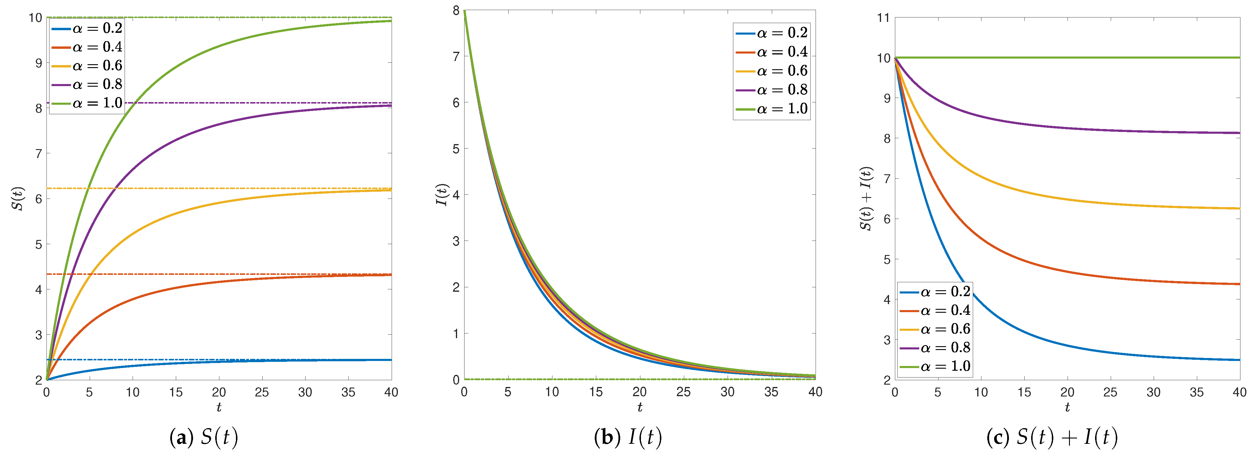
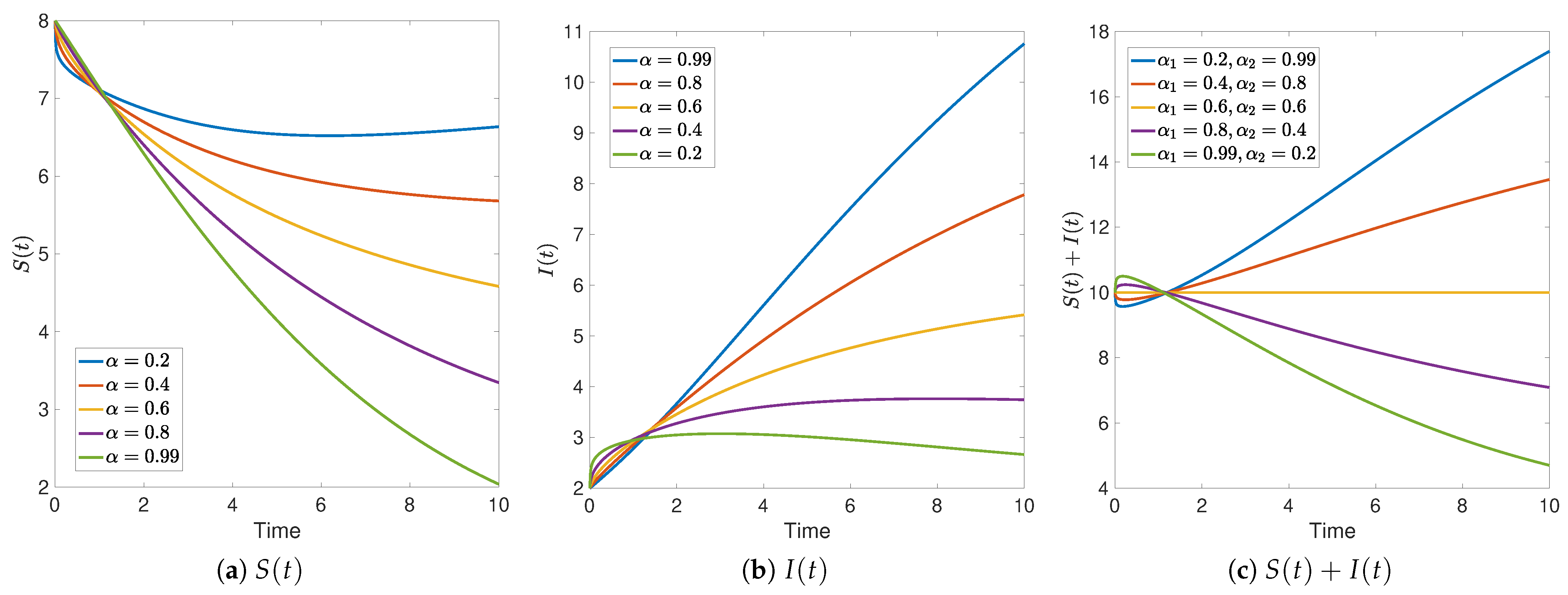
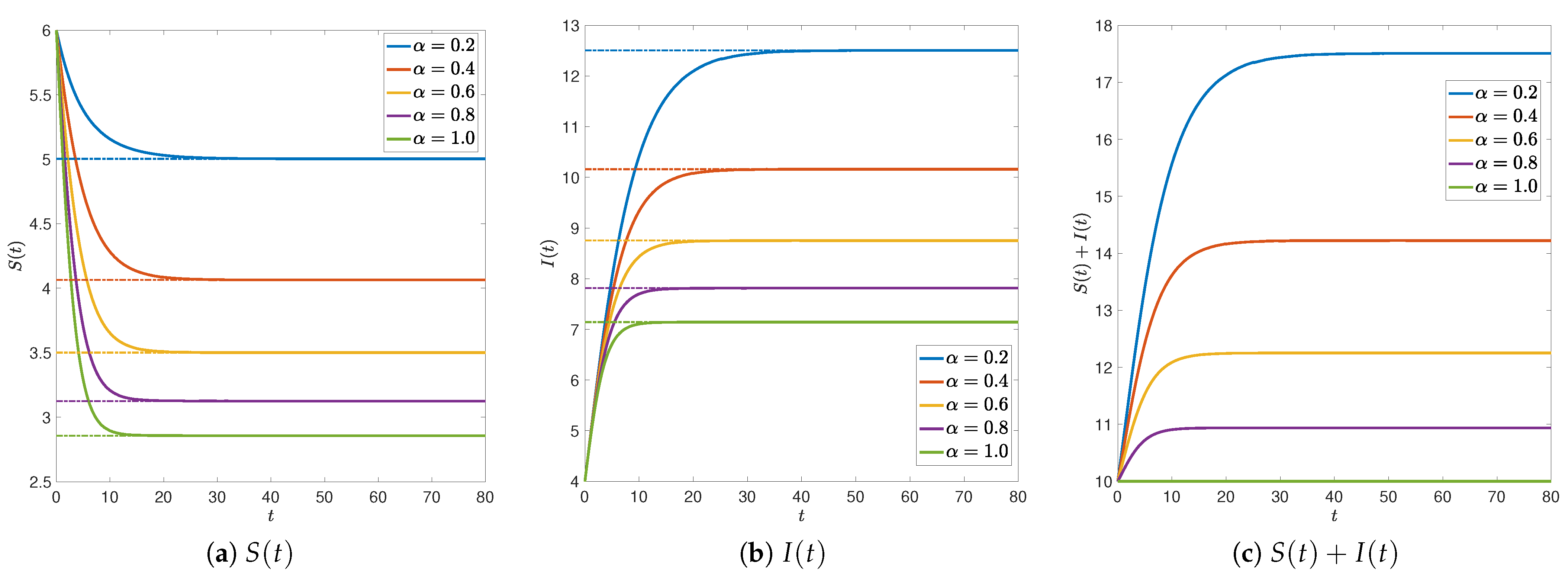
2.2. Numerical Simulations

The numerical discretization of system (1) follows [16]. Let us consider a general equation
C D t α u ( t ) = f ( u ( t ) )
and consider a numerical grid which uniformly divides the time interval [ 0 , T ] into N t steps of length Δ t . We denote by u n = u ( t n ) , with  t n = n Δ t . Let α ( 0 , 1 ) , then the Caputo derivative can be approximated as
C D t α u n = 1 Γ ( 2 α ) Δ t α u n j = 0 n 1 C n , j u j ,
with
C n , 0 = g ( n ) , C n , j = g ( n j ) g ( n ( j 1 ) ) for j = 1 , , n 1
and g ( n ) : = n 1 α ( n 1 ) 1 α for n 1 . The numerical scheme to solve (11) is then given by
u n + 1 = j = 0 n 1 C n , j u j + Γ ( 2 α ) Δ t α f ( u n ) .
Let us denote by S n = S ( t n ) and I n = I ( t n ) . By applying this discretization to system (1) we obtain
S n + 1 = j = 0 n 1 C n , j S j + Γ ( 2 α 1 ) Δ t α 1 f S ( S n , I n ) I n + 1 = j = 0 n 1 C n , j I j + Γ ( 2 α 2 ) Δ t α 2 ( f S ( S n , I n ) ) ,
with
f S ( S , I ) = β S S + I I + γ I .
We show the evolution in time of S ( t ) , I ( t ) and their sum S ( t ) + I ( t ) as α 1 , α 2 changes: in Figure 1 we considered a case with β > γ and in Figure 2 with γ < β . Note in plots (a) and (b) that the steepness of the solutions S ( t ) and I ( t ) in the long run are related to the size of α 1 and α 2 , respectively: this can be interpreted as a memory effect of the Caputo fractional operator [21]. An interesting phenomenon is also the lack of monotonicity of the solutions, in contrast with ordinary SIS models.
The sum of the two classes, see plots (c), shows that S ( t ) + I ( t ) is in general not monotone. For instance, in Figure 1, the total population S ( t ) + I ( t ) first decreases and then increases when α 1 > α 2 , while it first increases and then decreases when α 1 < α 2 (a symmetrical behavior emerges in Figure 2). in case α 1 = α 2 then the sum is constant and we recover the theory developed in [11,13]. A rigorous study of the symmetries emerging in the simulations and, in particular the intersections of all the functions N ( t ) at the same time, is still under investigation.

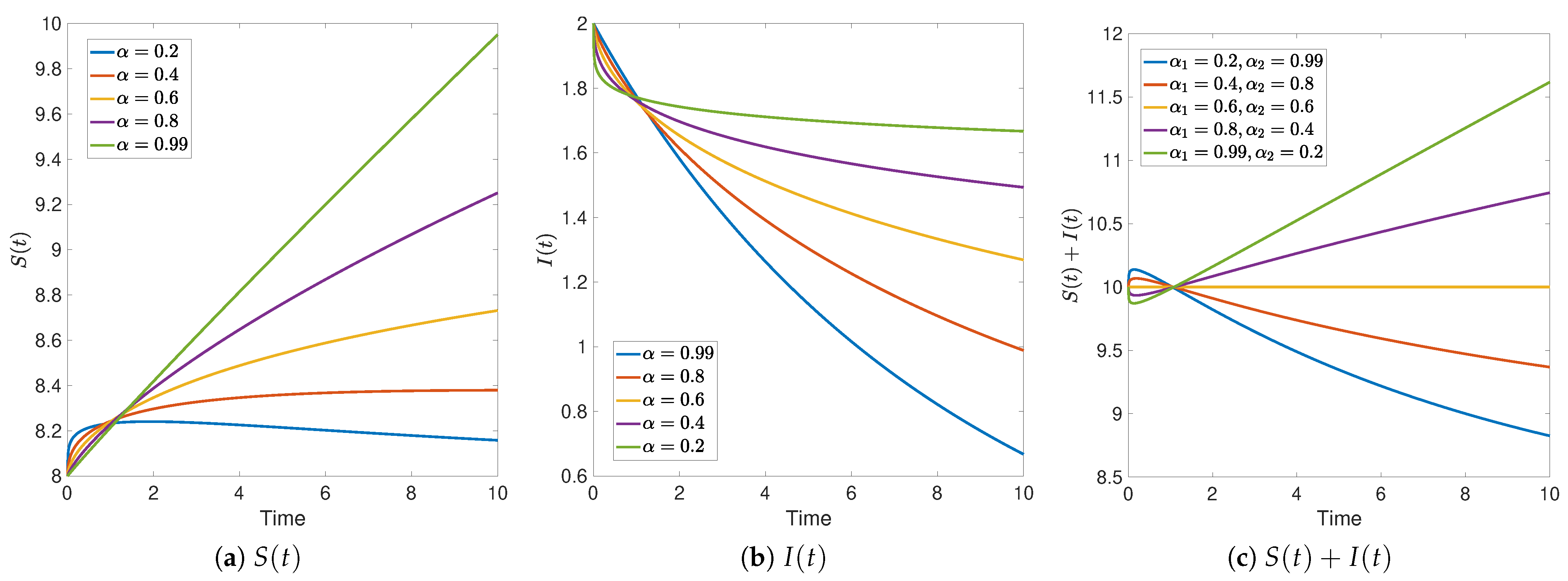
3. Caputo–Fabrizio Fractional Epidemic Models

In this section, we are concerned with the SIS model using Caputo–Fabrizio-type fractional derivatives. We refer to [22,23,24,25] for some examples of epidemic models based on the Caputo–Fabrizio fractional operator.
More precisely, here we study the fractionary SIS system (2). The identity
d d t CF D t α u ( t ) = M ( α ) 1 α u ( t ) α 1 α CF D t α u ( t ) t ( a , b ) , α ( 0 , 1 )
is crucial to reconduct (2) to a system of ordinary differential equations, which is the first step of our investigation.
We make the following key assumption, relating the order of derivation to the system parameters:
γ < α 1 α ,
M ( α ) α α ( 0 , 1 ] .
Note that, for any γ > 0 the condition (13) is satisfied by choosing α sufficiently close to 1 whereas (14) trivially holds by choosing M ( α ) 1 , which is a setting earlier explored and motivated in [26].

3.1. Solutions and Equilibria

As anticipated above, we begin by rewriting (2) as a system of ordinary equations for α [ 0 , 1 ) .
Theorem 2. 
Let α ( 0 , 1 ] , β , γ > 0 , S 0 , I 0 0 , I 0 + S 0 > 0 and assume the conditions (13) and (14). Let
B α : = 1 2 ( α + M ( α ) + ( 1 α ) ( β γ ) ) , C α : = M ( α ) ( α ( 1 α ) γ )
and
P α ( S 0 , I 0 ) : = M ( α ) S 0 + α I 0 + ( 1 α ) β γ β S 0 + I 0 I 0 I 0 .
Furthermore, define the function g α : R R
g α ( x ) : = B α x + P α ( S 0 , I 0 ) / 2 + ( B α x P α ( S 0 , I 0 ) / 2 ) 2 C α x 2 + M ( α ) P α ( S 0 , I 0 ) x ) M ( α ) .
Then any couple of non-negative absolutely functions continuous ( S ( t ) , I ( t ) ) is a solution of fractional system (2) if and only if
S ( t ) = g α ( I ( t ) ) t 0
and I ( t ) solves
I = β γ β I g α ( I ) + I I I ( 0 ) = I 0 .
Proof. 
Preliminarily remark that, by (12) and by the first equation of (2)
d d t D α CF S = M ( α ) 1 α S α 1 α D α C F S = M ( α ) 1 α S + α 1 α β S + I S γ I .
By differentiating both sides of the first equation of (2), we deduce that (2) is equivalent to the ordinary system
M ( α ) 1 α S + α 1 α β S + I S γ I = β S + I S γ I I = β S + I S γ I S ( 0 ) = S 0 I ( 0 ) = I 0 .
Now define
P ( t ) : = M ( α ) S ( t ) + α I ( t ) + ( 1 α ) β S ( t ) + I ( t ) S ( t ) γ I ( t ) = M ( α ) S ( t ) + α I ( t ) + ( 1 α ) β γ β S ( t ) + I ( t ) I ( t ) I ( t ) t 0
and remark that (17) implies P ( t ) = 0 and consequently P ( t ) = P ( 0 ) = P α ( S 0 , I 0 ) for all t 0 . Then, if  I ( t ) and S ( t ) are solutions of (17) (or equivalently, of (2)) then
M ( α ) S ( t ) + α I ( t ) + ( 1 α ) β γ β S ( t ) + I ( t ) I ( t ) I ( t ) = P α ( S 0 , I 0 ) .
By solving above equation with respect to S ( t ) and selecting the only possibly non-negative solution, we obtain for all t 0
S ( t ) = 1 M ( α ) B α I ( t ) + P α ( S 0 , I 0 ) / 2 + ( B α I ( t ) P α ( S 0 , I 0 ) / 2 ) 2 C α I 2 ( t ) + M ( α ) P α ( S 0 , I 0 ) I ( t ) = g α ( I ( t ) ) .
Incidentally notice that if α = 1 then P 1 ( I 0 ) = I 0 + S 0 = : N , B 1 = C 1 = 1 we recover from above relation the classical identity S ( t ) = N I ( t ) . We check that S ( t ) , as a function g α of I ( t ) , is well defined. To this end, note that g α ( x ) is defined in R , because 
( B α x P α ( S 0 , I 0 ) / 2 ) 2 C α x 2 + M ( α ) P α ( S 0 , I 0 ) x = ( B α 2 C α ) x 2 ( B α M α ) P α ( S 0 , I 0 ) x + P α 2 ( S 0 , I 0 ) / 4 0
for all x R . More precisely, above inequality holds because the discriminant of above polynomial reads
( B α M α ) 2 P α 2 ( S 0 , I 0 ) ( B α 2 C α ) P α 2 ( S 0 , I 0 ) = ( 1 α ) β M ( α ) P α 2 ( S 0 , I 0 ) < 0
for all α ( 0 , 1 ) , whereas we remarked above that if α = 1 then g α ( x ) = N x .
By plugging the identity S ( t ) = g α ( I ( t ) ) in the second equation of (2) we obtain (17).
Finally we check that S ( t ) and I ( t ) are non-negative. By (15), S ( t ) 0 if and only if I ( t ) [ 0 , P α ( S 0 , I 0 ) / ( α ( 1 α ) γ ) ] for all t 0 . Remark that this condition is satisfied for t = 0 , indeed we have
P α ( S 0 , I 0 ) α I 0 + ( 1 α ) ( β γ β S 0 + I 0 I 0 ) I 0 ( α ( 1 α ) γ ) I 0 .
Moreover if I ( t ) = P α ( S 0 , I 0 ) / ( α ( 1 α ) γ ) then I ( t ) = γ I ( t ) < 0 and, consequently I ( t ) P α ( S 0 , I 0 ) / ( α ( 1 α ) γ ) . Finally, remark that 0 is an equilibrium for (17) and that the velocity field f α ( I ) = β γ β I g α ( I ) + I I is locally Lipschitz continuous. Therefore, by the local uniqueness of the solutions of (17) if I 0 > 0 then I ( t ) > 0 for all t.    □

Equilibria

We now characterize the equilibria and we study the asymptotic behavior of (2).
Proposition 1. 
Let α ( 0 , 1 ] and assume conditions (13) and (14) and let S 0 , I 0 0 . The equilibria of the system (16) are 0 and
E α ( S 0 , I 0 ) : = ( β γ ) P α ( S 0 , I 0 ) α ( β γ ) + M ( α ) γ .
Setting R : = β / γ , E α ( I 0 ) > 0 if and only if R > 1 . in this case
I ( t ) E α ( S 0 , I 0 ) , S ( t ) γ β γ E α ( S 0 , I 0 ) = γ P α ( S 0 , I 0 ) α ( β γ ) + M ( α ) γ as t + .
Finally, if E α ( S 0 , I 0 ) 0 , that is if R 1 , then
I ( t ) 0 , S ( t ) P α ( S 0 , I 0 ) as t + .
Proof. 
The first part of the claim follows by a direct computation, using in particular (14) and the fact that β , γ > 0 implies R > 0 . Let x R = E α ( S 0 , I 0 ) if R > 1 and x R = 0 if R 0 . We proved in Theorem 2 that I ( t ) is non-negative, and consequently [ 0 , + ) is an invariant set for the dynamics (17). Moreover, by a direct computation one can check that the function V ( x ) : = ( x x R ) 2 is a Lyapunov function for (17) in [ 0 , + ) and, consequently, x R is a globally asymptotically stable equilibrium for (17) and this concludes the proof.    □
Note that, as in the classical case, the qualitative properties of the system strongly depend on the reproduction number R = β / γ . The value E α ( S 0 , I 0 ) can be seen as a fractional generalization of the endemic equilibrium of classical SIS models, which is a stable equilibrium when R > 1 .
The next result deals with the monotonicity and the asymptotic behavior of the function N ( t ) : = S ( t ) + I ( t ) , which is not constant unless we are in the ordinary case α = 1 . As we show below, the asymptotic behavior of N ( t ) can be used for inverse problems, i.e., to reconstruct the fractional order α of (2) from the observed data in the long range.
Proposition 2. 
Assume S 0 , I 0 > 0 and α ( 0 , 1 ) . If  R > 1 and if I 0 ( 0 , E ( S 0 , I 0 ) ) , then N ( t ) : = I ( t ) + S ( t ) is a strictly increasing function converging to
N α ( S 0 , I 0 ) : = β β γ E α ( S 0 , I 0 ) = β P α ( S 0 , I 0 ) α ( β γ ) + M ( α ) γ
as t + . Otherwise, if either R > 1 and I 0 > E α ( S 0 , I 0 ) or R 1 , then N ( t ) is strictly decreasing and tends to P α ( S 0 , I 0 ) / M ( α ) as t + .
Proof. 
We preliminary remark that g α ( x ) is a convex function; indeed
g α ( x ) = P α 2 ( S 0 , I 0 ) ( 1 α ) β 4 M ( α ) ( B α x P α ( S 0 , I 0 ) / 2 ) 2 C α x 2 + M ( α ) P α ( S 0 , I 0 ) 0 x R .
Moreover, by a direct computation,
1 + g α ( I 0 ) = 1 + 2 ( 1 α ) β M ( α ) ( I 0 + S 0 ) 3 P α ( S 0 , I 0 ) 2 I 0 ( I 0 + S 0 ) 2 + ( 1 α ) I 0 2 β 3 > 0
and this, together with the convexity of g α , implies
1 + g α ( x ) > 0 x I 0 .
Furthermore, remark that, using the assumption (14), i.e.,  M ( α ) α , we obtain
1 + g α ( E α ( S 0 , I 0 ) ) = 1 + M ( α ) ( 1 α ) ( β γ ) γ α β ( 1 α ) ( β γ ) 2 + β M ( α ) 1 + M ( α ) ( 1 α ) ( β γ ) γ β ( 1 α ) ( β γ ) 2 + β M ( α ) = ( 1 α ) ( β γ ) ( M ( α ) γ + β γ ) ( 1 α ) ( β γ ) 2 + β M ( α )
therefore
β > γ 1 + g α ( x ) > 0 x E 0 ( S 0 , I 0 ) .
We conclude this preliminary study on g α by noticing that
1 + g α ( 0 ) = ( 1 α ) ( 1 β + γ )
therefore
β γ 1 + g α ( x ) > 0 x 0 .
Now, by Theorem 2
N ( t ) = I ( t ) + S ( t ) = I ( t ) ( 1 + g α ( I ( t ) ) .
Assume R > 1 and I 0 ( 0 , E ( S 0 , I 0 ) ) . Then
I ( t ) = β γ β I ( t ) I ( t ) + g α ( I ( t ) ) I ( t ) > 0 t 0 .
In particular, I ( t ) I 0 for all t 0 , and, in view of (20) and (23), we deduce N ( t ) > 0 for all t > 0 ; hence, N ( t ) is strictly increasing.
Assume now that either R 1 or I 0 E ( S 0 , I 0 ) .
First we discuss the case in which R > 1 and I 0 > E ( S 0 , I 0 ) . Then I ( t ) < 0 , and, since E α ( S 0 , I 0 ) is a (globally asymptotically stable) equilibrium by Proposition 1, then I ( t ) > E α ( S 0 , I 0 ) for all t 0 . Then, in view of (21) and (23), we deduce N ( t ) < 0 for all  t 0 .
Finally, if  R 1 then I ( t ) < 0 . Since I ( t ) > 0 for all t > 0 then, in view of (22) and (23), we deduce N ( t ) < 0 for all t 0 , and this concludes the proof.    □
From the above result, we can estimate the fractional order α from the asymptotic behavior of the total population N ( t ) . Indeed, if  R > 1 and N ( t ) N , then the corresponding fractional order α is the solution of the equation
β P α ( S 0 , I 0 ) α ( β γ ) + M ( α ) γ = N .
By assuming, as in [26], M ( α ) 1 , and setting N 0 : = I 0 + S 0 , the above equation reduces to the explicit formula
α = 1 ( N N 0 ) N 0 β β I 0 S 0 β N 0 ( I 0 + γ I 0 N ) γ N 0 N .
Note in particular that α = 1 if and only if N = N 0 , confirming the fact that, in the proposed mixed fractional model, N ( t ) is constant if and only if α = 1 .

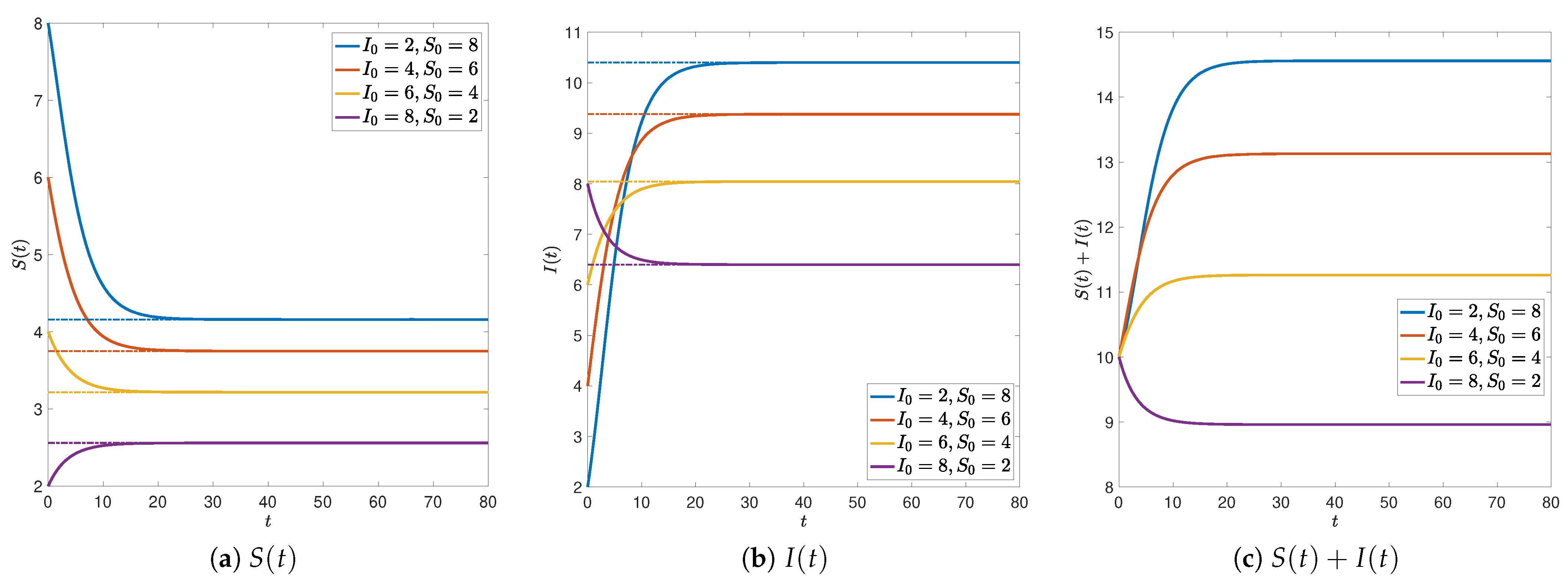
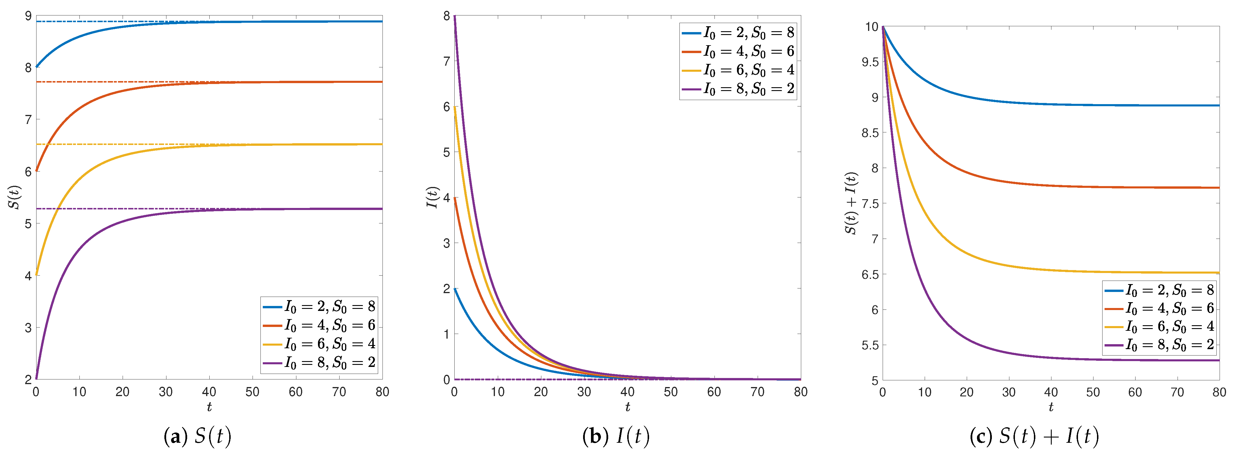
3.2. Numerical Simulations

The numerical discretization of (2) is based on the results of Theorem 2. Let us consider again the numerical grid introduced in Section 2.2. To compute the discrete evolution in time of I and S we first solve system (16) by a proper ODE solver and then we discretize (15). Specifically, we use the MATLAB tool ode23t to compute I n + 1 and then, following (15), we obtain S n + 1 = g α ( I n + 1 ) .
In Figure 3 and Figure 4 we show the results obtained as α changes in { 0.2 , 0.4 , 0.6 , 0.8 , 1 } . The parameters S 0 , I 0 , M ( α ) and γ are the same in all simulations, fixed as S 0 = 6 , I 0 = 4 , M ( α ) 1 and γ = 0.2 . The parameter β , instead, is set to β = 0.7 in Figure 3, which implies R > 1 , while β = 0.1 in Figure 4, and thus R < 1 . The dashed lines represent the equilibria estimated in Proposition 1. Both S and I monotonically converge to their equilibria. Note that the time delay induced by the fractional order emerges in the fact that the smallest is α , the slowest is the convergence of the related solutions to equilibria. Finally, remark that, for α = 1 , the sum N ( t ) = S ( t ) + I ( t ) is constant, since (2) coincides with the classical SIS model, while if α < 1 , then the monotonicity of N ( t ) is in agreement with Theorem 2.
In Figure 5 and Figure 6, we fix α = 0.5 and we set S 0 = 10 I 0 and let the initial data I 0 vary in { 2 , 4 , 6 , 8 } . We note that the qualitative behavior of the solutions is in agreement with the theory developed here, and it is not much affected by initial data.

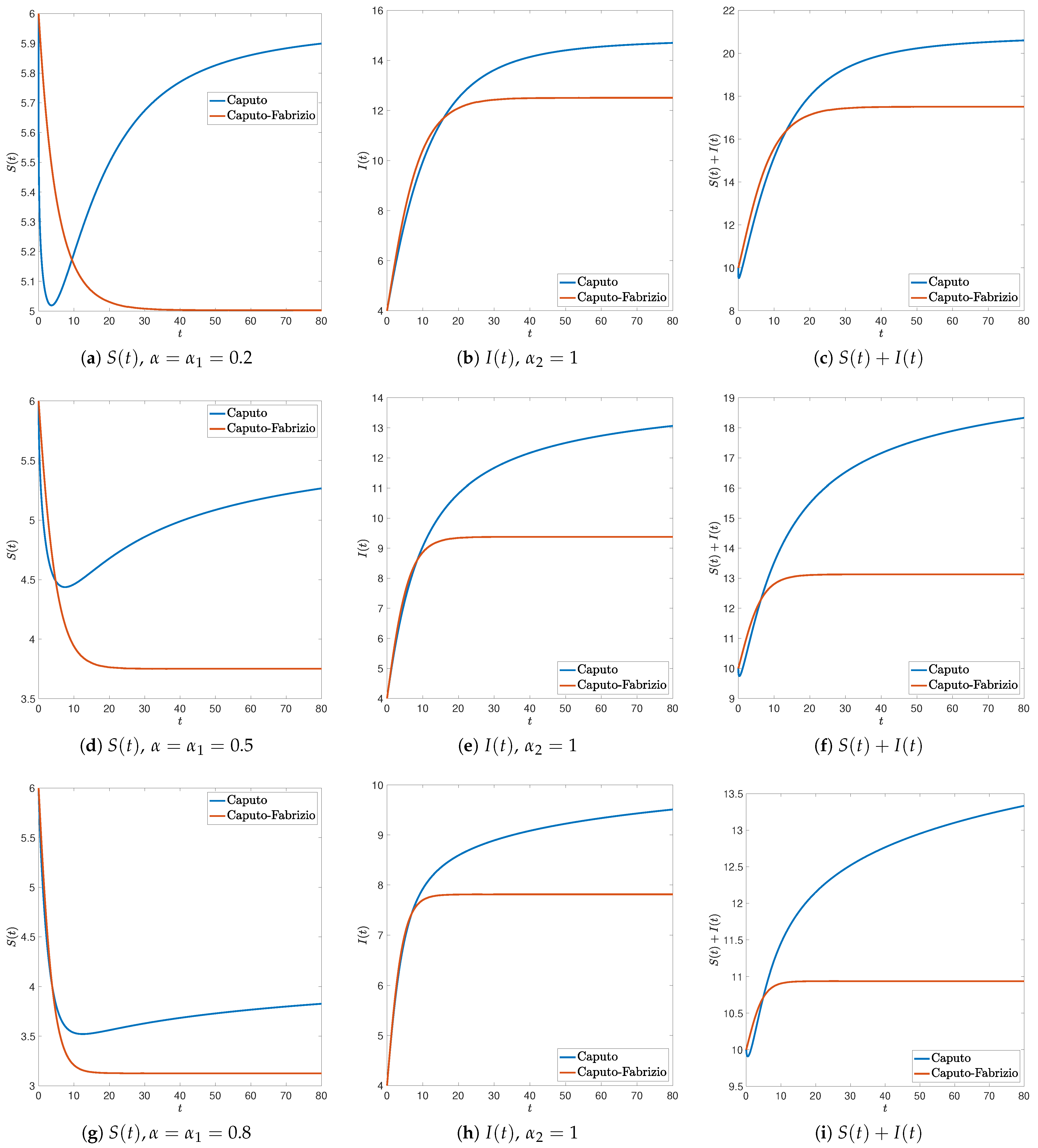
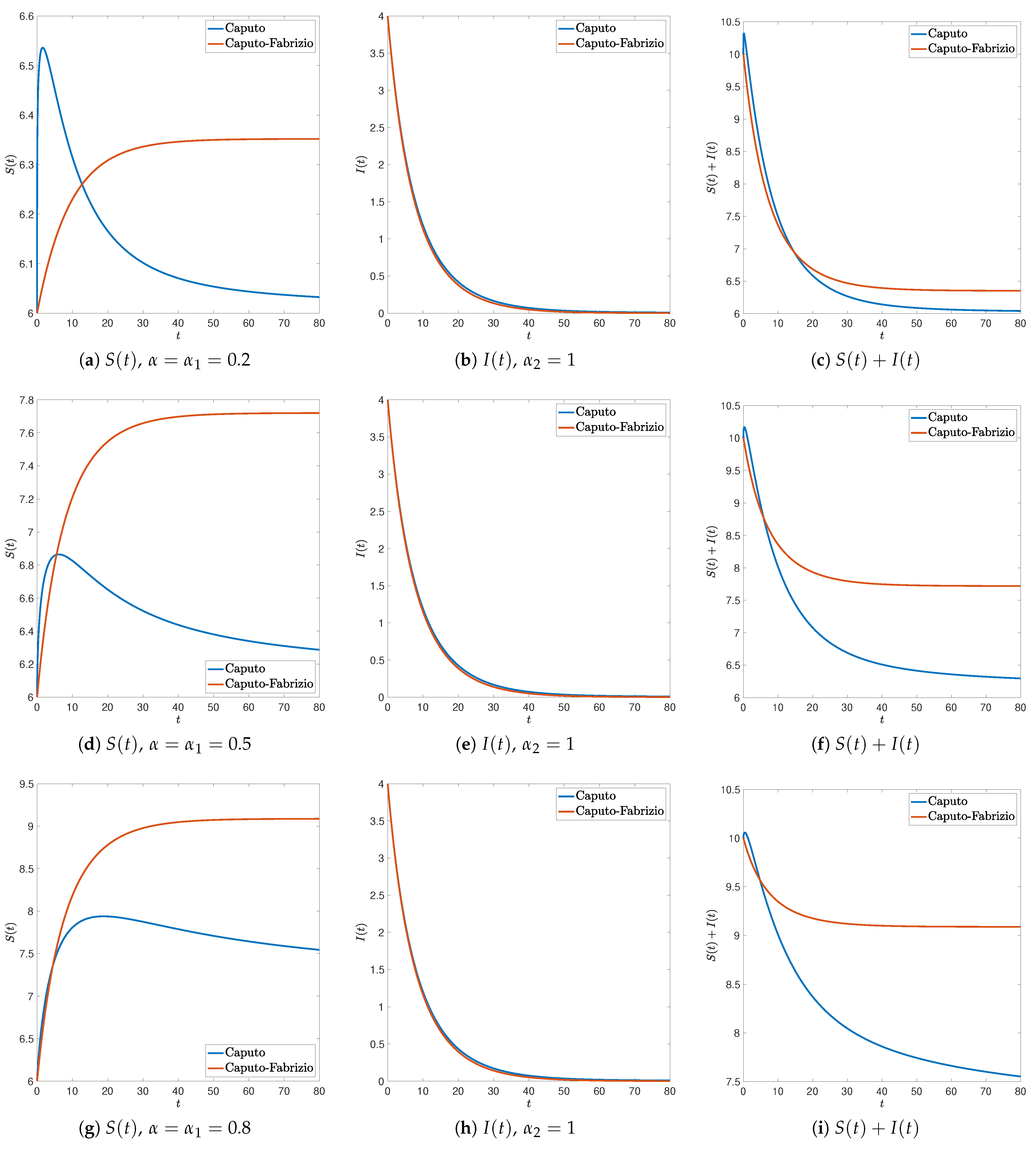
Comparison between Caputo SIS Model and Caputo–Fabrizio SIS Model

We conclude this section with some tests pointing out the effect of the choice of a particular fractional operator on SIS models. We directly compare the numerical solution to the system with Caputo fractional SIS model (1) and Caputo–Fabrizio fractional SIS model (2). To this end, we fix the initial data S 0 = 6 and I 0 = 4 . We consider the set the fractional orders α 1 and α 2 in (1), the fractional order α in (2), and we set α 1 = α , α 2 = 1 , letting α vary in the set { 0.2 , 0.5 , 0.8 } . Figure 7 depicts the results in a case with γ < β , in particular γ = 0.2 and β = 0.7 , whereas in Figure 8, we test a case with β < γ , in particular γ = 0.2 and β = 0.1 . Note that the evolution of susceptible population S ( t ) is mostly affected by the change of differential operator, and this effect is augmented by choosing small fractional orders. Finally, note that the Caputo–Fabrizio operator preserves the monotonicity properties of the ordinary SIS case, while the Caputo operator used in (1) yields a more complex structure.

4. Conclusions

We explored the effects of fractional differential operators on SIS epidemic models. The main novelty of the present paper consists in letting the susceptible and the infected population evolve with different orders of fractional differential operators and the setting in a mathematical framework of these generalized models. Not only is our work based on numerical simulations, but we also tried to give some mathematical answers, and we used the numerical simulations to complete the investigation. We presented two fractional SIS models with mixed fractional orders. One of them involves the Caputo fractional derivative, characterized by a singular, power-law kernel. The other proposed model relies on the recently introduced Caputo–Fabrizio differential operator, which has a non-singular, exponential kernel.
For both models we established existence results for the solutions, and we conducted a qualitative analysis by means of numerical simulations. In the case of the Caputo–Fabrizio operator, under the assumption that the fractional behavior is restricted to the susceptible population whereas the infected population evolves according to an ordinary differential equation, we were able to take some further steps in the analysis of the system. Indeed, we characterized the equilibria, noticed their strong dependence on the reproduction number according to classical theory, and proposed a method for inverse problems. Finally, we numerically, directly compared the proposed Caputo and Caputo–Fabrizio SIS models, in order to let the effects of each particular differential operator on the system emerge. We remark that the numerical simulations of the Caputo-type model showed a non-monotone nature of the solutions for small values of one of the two fractional orders. The sum of infected and susceptible populations is not constant, suggesting that the vital dynamics are hidden in the mixed fractional orders, and this fact deserves further investigations. The tests related to the Caputo–Fabrizio model confirm the theoretical results developed in Section 3. The two types of fractional derivative are finally compared in section, where we observed again the lack of monotonicity of Caputo solutions, in contrast to the monotonicity shown by Caputo–Fabrizio solutions.
We believe that the possibility of tuning the memory effects in a single compartment of the population (susceptible/infected) by means of ad hoc fractional orders may provide finer and effective tools in data fitting and mathematical modeling of epidemic dynamics.
Further possible extensions of the present work include the extension of the proposed methods to other epidemic models, for instance, the SIR model, and to controlled, mixed fractional epidemic dynamics.

Author Contributions

Conceptualization; methodology; software; validation; formal analysis; investigation; writing—original draft preparation; writing—review and editing: C.B., M.D., A.C.L. and P.L. All authors have read and agreed to the published version of the manuscript.

Funding

This research was partially supported by Progetto Ateneo Sapienza Università di Roma "Fractional derivatives in Science and Engineering”, grant number RM118164367E9B16.

Data Availability Statement

Data is contained within this article.

Conflicts of Interest

The authors declare no conflict of interest.

References

  1. Kermack, W.O.; McKendrick, A.G. A contribution to the mathematical theory of epidemics. Proc. R. Soc. Lond. Ser. A 1927, 115, 700–721. [Google Scholar]
  2. Hethcote, H.W. Three basic epidemiological models. In Applied Mathematical Ecology (Trieste, 1986); Biomathematics; Springer: Berlin, Germany, 1989; Volume 18, pp. 119–144. [Google Scholar] [CrossRef]
  3. Chen, Y.; Liu, F.; Yu, Q.; Li, T. Review of fractional epidemic models. Appl. Math. Model. 2021, 97, 281–307. [Google Scholar] [CrossRef] [PubMed]
  4. Deng, W.; Li, C.; Lü, J. Stability analysis of linear fractional differential system with multiple time delays. Nonlinear Dyn. 2007, 48, 409–416. [Google Scholar] [CrossRef]
  5. Yavuz, M.; Sene, N. Stability analysis and numerical computation of the fractional predator–prey model with the harvesting rate. Fractal Fract. 2020, 4, 35. [Google Scholar] [CrossRef]
  6. Daşbaşi, B. Stability analysis of the hiv model through incommensurate fractional-order nonlinear system. Chaos Solitons Fractals 2020, 137, 109870. [Google Scholar] [CrossRef]
  7. Caputo, M. Linear models of dissipation whose Q is almost frequency independent—II. Fract. Calc. Appl. Anal. 2008, 11, 4–14, reprinted in Geophys. J. Int. 1967, 13, 529–539. [Google Scholar] [CrossRef]
  8. Verhulst, P.F. Notice sur la loi que la population suit dans son accroissement. Corresp. Math. Phys. 1838, 10, 113–126. [Google Scholar]
  9. Verhulst, P.F. Recherches mathématiques sur la loi d’accroissement de la population. J. Econ. 1845, 12, 276. [Google Scholar]
  10. Verhulst, P.F. Deuxième mémoire sur la loi d’accroissement de la population. Mémoires De L’académie Royale des Sciences des Lettres et des Beaux-Arts de Belgique 1847, 20, 1–32. [Google Scholar]
  11. Balzotti, C.; D’Ovidio, M.; Loreti, P. Fractional SIS Epidemic Models. Fractal Fract. 2020, 4, 44. [Google Scholar] [CrossRef]
  12. El-Saka, H. The fractional-order SIR and SIRS epidemic models with variable population size. Math. Sci. Lett. 2013, 2, 195. [Google Scholar] [CrossRef]
  13. Hassouna, M.; Ouhadan, A.; El Kinani, E.H. On the solution of fractional order SIS epidemic model. Chaos Solitons Fractals 2018, 117, 168–174. [Google Scholar] [CrossRef] [PubMed]
  14. D’Ovidio, M.; Loreti, P. Solutions of fractional logistic equations by Euler’s numbers. Phys. A 2018, 506, 1081–1092. [Google Scholar] [CrossRef] [Green Version]
  15. Brauer, F.; Castillo-Chavez, C.; Feng, Z. Mathematical Models in Epidemiology; Texts in Applied Mathematics; Springer: New York, NY, USA, 2019; Volume 69. [Google Scholar] [CrossRef]
  16. Giga, Y.; Liu, Q.; Mitake, H. On a discrete scheme for time fractional fully nonlinear evolution equations. Asymptot. Anal. 2020, 120, 151–162. [Google Scholar] [CrossRef] [Green Version]
  17. Caputo, M.; Fabrizio, M. A new definition of fractional derivative without singular kernel. Progr. Fract. Differ. Appl. 2015, 1, 1–13. [Google Scholar]
  18. Kumar, D.; Singh, J.; Al Qurashi, M.; Baleanu, D. A new fractional SIRS-SI malaria disease model with application of vaccines, antimalarial drugs, and spraying. Adv. Differ. Equ. 2019, 2019, 278. [Google Scholar] [CrossRef] [Green Version]
  19. Yavuz, M.; Özdemir, N. Analysis of an epidemic spreading model with exponential decay law. Math. Sci. Appl. E-Notes 2020, 8, 142–154. [Google Scholar] [CrossRef] [Green Version]
  20. Coddington, E.A.; Levinson, N. Theory of Ordinary Differential Equations; Tata McGraw-Hill Education: New Delhi, India, 1955. [Google Scholar]
  21. Mainardi, F.; Gorenflo, R. Time-fractional derivatives in relaxation processes: A tutorial survey. Fract. Calc. Appl. Anal. 2007, 10, 269–308. [Google Scholar]
  22. Higazy, M.; Alyami, M.A. New Caputo-Fabrizio fractional order SEIASqEqHR model for COVID-19 epidemic transmission with genetic algorithm based control strategy. Alex. Eng. J. 2020, 59, 4719–4736. [Google Scholar] [CrossRef]
  23. Khan, S.A.; Shah, K.; Kumam, P.; Seadawy, A.; Zaman, G.; Shah, Z. Study of mathematical model of Hepatitis B under Caputo-Fabrizo derivative. AIMS Math. 2021, 6, 195–209. [Google Scholar] [CrossRef]
  24. Moore, E.J.; Sirisubtawee, S.; Koonprasert, S. A Caputo-Fabrizio fractional differential equation model for HIV/AIDS with treatment compartment. Adv. Differ. Equ. 2019, 200, 20. [Google Scholar] [CrossRef] [Green Version]
  25. Ullah, S.; Khan, M.A.; Farooq, M.; Hammouch, Z.; Baleanu, D. A fractional model for the dynamics of tuberculosis infection using Caputo-Fabrizio derivative. Discret. Contin. Dyn. Syst. Ser. S 2020, 13, 975–993. [Google Scholar] [CrossRef] [Green Version]
  26. Losada, J.; Nieto, J.J. Properties of a new fractional derivative without singular kernel. Progr. Fract. Differ. Appl 2015, 1, 87–92. [Google Scholar]
Figure 1. Numerical solutions to (1) with β = 0.7 , γ = 0.2 , I 0 = 2 and S 0 = 8 .
Computation 09 00089 g001
Figure 2. Numerical solutions to (1) with β = 0.1 , γ = 0.2 , I 0 = 8 and S 0 = 2 .
Computation 09 00089 g002
Figure 3. Numerical solutions to (2) for β = 0.7 , γ = 0.2 , S 0 = 6 , I 0 = 4 , and M ( α ) 1 as α changes.
Computation 09 00089 g003
Figure 4. Numerical solutions to (2) with β = 0.1 , γ = 0.2 , S 0 = 6 , I 0 = 4 , and M ( α ) 1 as α changes.
Computation 09 00089 g004
Figure 5. Numerical solutions to (2) for α = 0.5 , β = 0.7 , γ = 0.2 and M ( α ) 1 as I 0 and S 0 change.
Computation 09 00089 g005
Figure 6. Numerical solutions to (2) for α = 0.5 , β = 0.1 , γ = 0.2 and M ( α ) 1 as I 0 and S 0 change.
Computation 09 00089 g006
Figure 7. Numerical solutions to (1) and (2) for α = α 1 = 0.2 (top), α = α 1 = 0.5 (center), and α = α 1 = 0.8 (bottom) with α 2 = 1 , β = 0.7 , γ = 0.2 , S 0 = 6 , I 0 = 4 and M ( α ) 1 .
Computation 09 00089 g007
Figure 8. Numerical solutions to (1) and (2) for α 1 = 0.2 (top), α 1 = 0.5 (center) and α 1 = 0.8 (bottom) with α 2 = 1 , β = 0.1 , γ = 0.2 , S 0 = 6 , I 0 = 4 and M ( α ) 1 .
Computation 09 00089 g008
Publisher’s Note: MDPI stays neutral with regard to jurisdictional claims in published maps and institutional affiliations.

