Improvement and Assessment of a Blind Image Deblurring Algorithm Based on Independent Component Analysis

Abstract

The aim of the present paper is to improve an existing blind image deblurring algorithm, based on an independent component learning paradigm, by manifold calculus. The original technique is based on an independent component analysis algorithm applied to a set of pseudo-images obtained by Gabor-filtering a blurred image and is based on an adapt-and-project paradigm. A comparison between the original technique and the improved method shows that independent component learning on the unit hypersphere by a Riemannian-gradient algorithm outperforms the adapt-and-project strategy. A comprehensive set of numerical tests evidenced the strengths and weaknesses of the discussed deblurring technique.

1. Introduction

Deblurring a grey-scale image consists in recovering a sharp image on the basis of a single blurred observation (possibly corrupted by disturbances). Blurring artifacts are caused by defocus aberration or motion blur [1]. In the case of uniform defocus blur, the physical process that leads to a defocused image is typically modeled by convolution of the original image with a point-spread function (PSF) plus additive noise [2]. The left-hand side of Figure 1 shows a schematic of such model, where the original image intensity is denoted by f and the blurred image intensity is denoted by g. A closely related problem is blind deblurring from more than a single out-of-focus observation of a sharp image [3]. Motion blur may be modeled as the integration over a light field captured at each time during exposure [4].

Whenever the PSF is known a priori, it is possible to invoke several deblurring algorithms that afford reconstructing the original image; otherwise, it is difficult to estimate the PSF and the original image intensity simultaneously. A class of algorithms, known as blind deblurring methods, afford the simultaneous estimation of the PSF and the original image intensity. Indeed, blind deblurring derives from blind deconvolution, a method capable of undoing convolution with an unknown function [5,6]. Deblurring algorithms are used in astronomy [7], where it is necessary to treat photographic images taken by terrestrial telescopes whose quality is degraded by atmospheric turbulence. Blind deblurring of out-of-focus recorded images is also part of barcode and QR-code processing [8,9].

Over the years, blind deconvolution algorithms have been widely utilized, especially in mono-dimensional voice/sound signal deconvolution (as in communication channels to eliminate intersymbol interference or in sound recording to eliminate reverberation). In [10,11], mono-dimensional deconvolution is extended to bi-dimensional signal deconvolution that affords recovering an image from one of its blurred observations without the need to know the PSF. In fact, the author of [10,11] proposed the application of Gabor filters to a blurred image to decompose a single source image into a number of filtered pseudo-images, as shown in the central part of Figure 1. Such pseudo-images, together with the source image, are utilized as inputs to an independent component analysis (ICA) algorithm. Under appropriate hypotheses, the first independent component, denoted as $f^{\prime }$ in Figure 1, may be proven to represent an estimation of the original image f up to inessential scaling.

Gabor and Gabor-like filters are instrumental in a large number of image processing techniques, as testified by the abundant literature in the field (see, e.g., [12,13]). Likewise, independent component analysis is a statistical information processing method that has found widespread applications in sciences and engineering (see, e.g., [14,15,16,17,18,19,20].

In the contributions [10,11] by Umeyama, the ICA method utilized to separate the original image out from its blurred version is implemented by an adapt-and-project neural-learning algorithm. The present paper aims at modifying the original adapt-and-project neural-learning ICA algorithm by an exponentiated-gradient learning on the unit hypersphere and evaluating the ability of such algorithm in learning the first independent component from a set of pseudo-images so as to recover the original sharp image. In addition, the present paper illustrates comparative results with respect to the original method and discusses its strengths and weaknesses through a comprehensive set of experiments performed on synthetic as well as real-world datasets.

Ultimately, the present paper summarizes a research work carried out by the author out of curiosity to review and evaluate an older—and cleverly designed—blind image deblurring algorithm by Umeyama. As such, the present paper does not claim any superiority to current state-of-the-art methods (such as DeblurGAN or DeblurGAN-2 [21,22]). State-of-the-art algorithms are certainly much more involved and better performing than a two-equation-based algorithm such as Umeyama’s and one may safely take for granted that new algorithms are incomparably better than the one discussed in the present paper. For these reasons, no comparisons with further existing algorithms were carried out in the context of the present paper.

Manifold calculus (an abridgement for ‘calculus on manifold’) is a branch of mathematics that lies at the intersection of mathematical analysis, geometry, topology and algebra [23]. Manifold calculus turned out to represent the natural language of curved spaces, such as the sphere and the hyper-sphere, as well as of non-Euclidean spaces, namely continuous sets endowed with a non-Euclidean distance function. Manifold calculus proves extremely effective in formulating scientific problems subjected to non-linear (holonomic) constraints and designing numerical algorithms to solve such problems with applications to computational mechanics [24], biomedical engineering [25], electrical engineering [26] and aerospace engineering [27].

The present paper is organized as follows. Section 2 recalls the original theory by Umeyama and introduces an improved neural learning algorithm designed by means of manifold calculus. Section 3 presents several numerical experiments to validate the proposed learning algorithm, which were performed on synthetic test-images as well as on real-world blurred images. Section 4 concludes the paper.

2. Theoretical Developments and Methods

The present section summarizes theoretical tools that are instrumental in the development of an ICA-based blind image deblurring algorithm, namely Gabor filters in Section 2.1, blurred-image modeling by convolution by a point-spread function and by Taylor series expansion in Section 2.2 and an adapt-and-project neural-ICA algorithm in Section 2.3. In addition, this section introduces an exponentiated-gradient independent component learning method in Section 2.4.

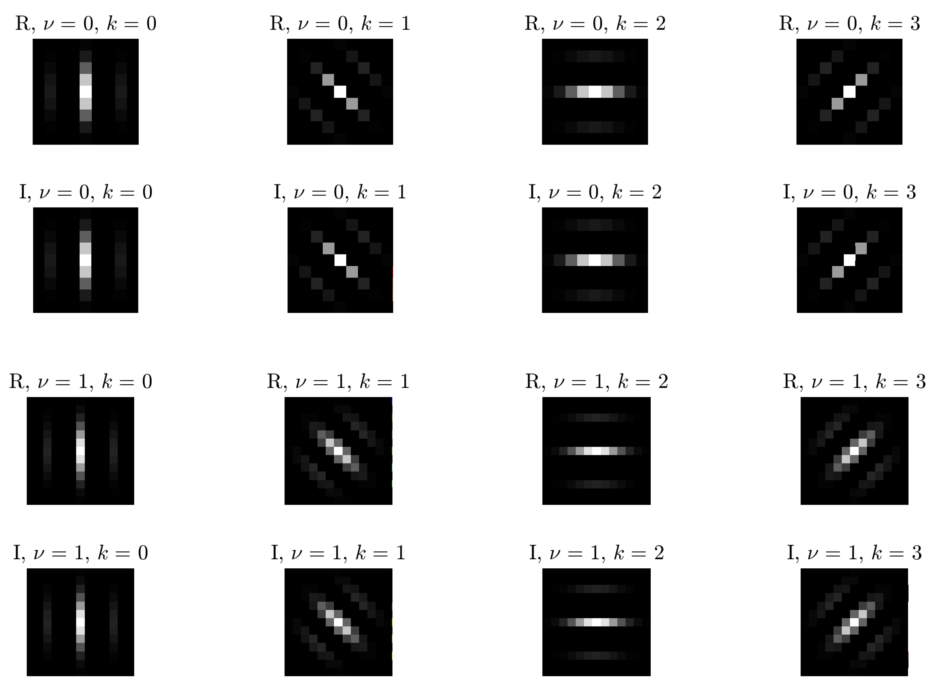
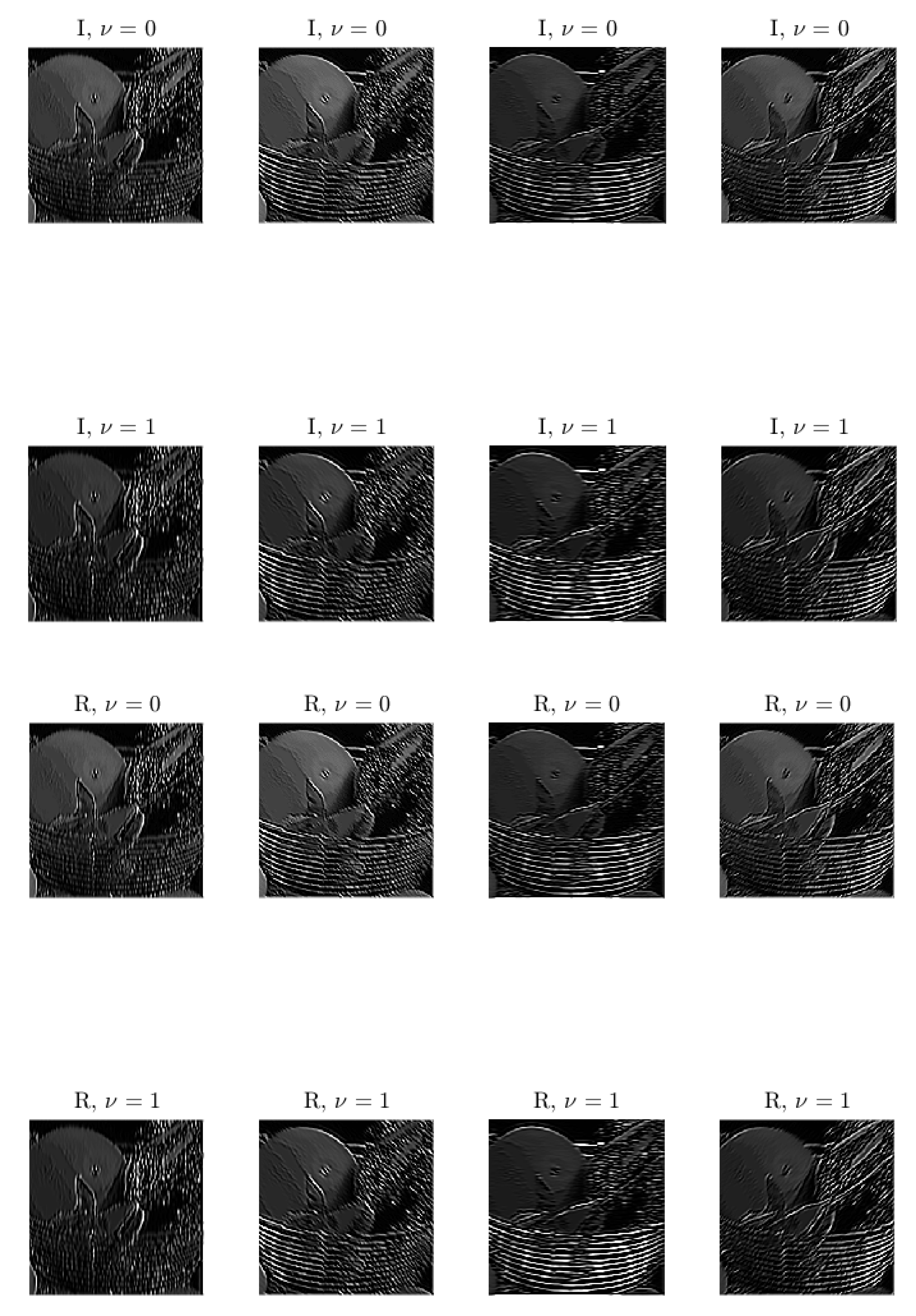
2.1. Bi-Dimensional Gabor Filters

Gabor filters, widely employed in computer vision, realize multichannel filters that can decompose an image into a number of filtered pseudo-images [28]. Bi-dimensional Gabor filters are constructed as the product of a Gaussian bell function and a planar wave that propagates on a bi-dimensional plane. Each Gabor filter is therefore unequivocally determined by the standard deviation of a Gaussian function, the direction of propagation and the wavelength of the associated planar wave.

A bi-dimensional Gabor filter is defined as a complex-valued function whose real and imaginary parts are conceived as two distinct real-valued filters:

$$\left\{\begin{array}{c}R(x,y;\nu ,k):=exp\left(-\frac{x^2+y^2}{2{{\sigma }_{\nu }}^2}\right)cos\frac{\pi }{{\sigma }_{\nu }}\left(xcos{\varphi }_k+ysin{\varphi }_k\right),\hfill \\ I(x,y;\nu ,k):=exp\left(-\frac{x^2+y^2}{2{{\sigma }_{\nu }}^2}\right)sin\frac{\pi }{{\sigma }_{\nu }}\left(xcos{\varphi }_k+ysin{\varphi }_k\right),\hfill \end{array}\right.$$

(1)

where a pair $(x,y)$ denotes the location of a pixel in an image in the form x = column-index and y = row-index; ${\sigma }_{\nu }:=2^{\frac{\nu +1}{2}}$ defines the standard deviation of the Gaussian bell as well the wavelength of the planar wave; and ${\varphi }_k:=\frac{\pi }{4}k$ defines the direction of propagation. The size of a Gabor filter in pixel unit is denoted by G, namely $x,y\in \left\{-G,\dots ,0,\dots ,G\right\}$.

Figure 2 shows a set of Gabor filters corresponding to the parameters values $\nu \in \left\{0,1\right\}$ and $k\in \left\{0,1,2,3\right\}$. Such combination gives rise to eight complex-valued Gabor filters that correspond to 16 real-valued Gabor filters defined in Equation (1). The first two rows of Figure 2 show Gabor filters corresponding to $\nu =0$, while the last rows show filters obtained upon setting $\nu =1$. The first and third rows show the filters $R(x,y;\nu ,k)$, which mimic the response of a simple biological neuron tuned to respond to a straight line, while the second and fourth rows show the filters $I(x,y;\nu ,k)$, which mimic the response of a neuron tuned to edges.

2.2. A Blurred Image Model Based on Taylor Series Expansion

In the present work, we assume the blur to be uniform, in which case the underlying physical process that leads to a blurred recording of a sharp image may be modeled by bi-dimensional convolution between the sharp image intensity $f(x,y)$ and a point-spread function $h(x,y)$. In short notation, with reference to Figure 1, $g:=f\otimes h$ holds. Non-uniform blurring may be coped with by estimating the unknown blur-field [2]. In the present work, we ignore the unpredictable additive disturbance due, for example, to atmospheric particulate matter that might affect the quality of image recording, since additive noise in the model may be mitigated by dedicated pre-processing algorithms [29].

According to the above-recalled convolutional model, the brightness (or intensity) of a pixel in the blurred image $g(x,y)$ is calculated as:

$$g(x,y)=\sum _{s=-M}^M\sum _{t=-M}^{M}h(s,t)f(x+s,y+t),$$

(2)

where M represents the spatial extension of the point-spread function ($2M+1$ pixels in both dimensions). The notation $f(x+s,y+t)$ indicates the intensity of a pixel adjacent to the location $(x,y)$ by an offset $(+s,+t)$.

A key observation that affords linking blind image deblurring to independent component analysis is that the intensity $f(x+s,y+t)$ may be expressed in terms of the intensity $f(x,y)$ of the central pixel and of its spatial derivatives $f_x(x,y)$ and $f_y(x,y)$ through Taylor expansion, namely:

$$f(x+s,y+t)=f(x,y)+\alpha (s{f}_x(x,y)+t{f}_y(x,y))+\dots .$$

(3)

The above expression is indeed based on a slight abuse of notation caused by an identification of the discrete function f with its linearly extended continuous version to which Taylor series may be applied. Such analytic extension requires spatial sampling represented by the coefficient $\alpha >0$ (which may be safely taken equal to 1 in the computer implementation or absorbed into other constants).

Replacing the value of the intensity $f(x+s,y+t)$ in the convolutional model (2) by its Taylor series representation (3), the intensity $g(x,y)$ may be approximated as follows:

$$g(x,y)=a_{1}f(x,y)+a_2{f}_x(x,y)+a_3{f}_y(x,y)+\dots ,$$

(4)

where

$$\left\{\begin{array}{c}{a}_1:={\sum }_{s=-M}^M{\sum }_{t=-M}^{M}h(s,t),\hfill \\ a_2:=\alpha {\sum }_{s=-M}^M{\sum }_{t=-M}^{M}sh(s,t),\hfill \\ a_3:=\alpha {\sum }_{s=-M}^M{\sum }_{t=-M}^{M}th(s,t).\hfill \end{array}\right.$$

(5)

The relationship (4) shows that the recorded image g may be thought of as a linear superposition of the original sharp image f and of its derivatives, since the convolutional model $g=f\otimes h$ is linear.

As a consequence, it is conceivable to recover the first term from the sum (4) by operating a linear combination of pixel-intensity values that cancels out the higher-order terms. Since the function f is unknown, the higher-order terms in the right-hand side of the relationship (4) are likewise unknown. Under the hypothesis that the pixel-intensity values and their derivatives are independent from one another, the sought linear combination that is able to separate out the first term from the higher-order term may be learned adaptively by a neural independent component analysis algorithm (for a survey on independent component analysis, see, e.g., [30]).

In order to feed an independent component analysis neural network with enough information to operate the separation of the sharp component from higher-order components, it is necessary to augment the available recordings (from one to many). Data augmentation may be obtained by use of the bi-dimensional Gabor filters recalled in Section 2.1. Model-wise, applying a number of Gabor filters to a blurred image is equivalent to considering the original image to be convoluted by a filter that, in turns, results from the convolution between a Gabor filter and a point-spread function, namely $h^{\prime }:=R\otimes h$ or $h^{\prime }=I\otimes h$, where R and I denote the Gabor filter functions introduced in Section 2.1. An example of a blurred image filtered by the 16 Gabor filters shown in Figure 2 is illustrated in Figure 3.

The Gabor-filtered image is, in short notation, denoted by $g^{\prime }:=h^{\prime }\otimes f$. The intensity value of each Gabor-filtered pseudo-image may thus be written as

$$g^{\prime }(x,y)=a_1^{\prime }f(x,y)+a_2^{\prime }{f}_x(x,y)+a_3^{\prime }{f}_y(x,y)+\dots$$

(6)

where we introduce the coefficients

$$\left\{\begin{array}{c}{a}_1^{\prime }:={\sum }_{s=-M}^M{\sum }_{t=-M}^M{h}^{\prime }(s,t),\hfill \\ a_2^{\prime }:=\alpha {\sum }_{s=-M}^M{\sum }_{t=-M}^{M}s{h}^{\prime }(s,t),\hfill \\ a_3^{\prime }:=\alpha {\sum }_{s=-M}^M{\sum }_{t=-M}^{M}t{h}^{\prime }(s,t).\hfill \end{array}\right.$$

(7)

The coefficients $a_i^{\prime }$ depend on the shape of the applied Gabor filters.

The relationship (6) shows that the Gabor-filtered blurred image $g^{\prime }$ may be expressed again as a linear superposition of the original sharp image f and of its higher-order spatial derivatives. Hence, feeding a set of Gabor-filtered blurred images to a neural independent component analysis algorithm might result in recovering the original image, provided the sharp image and its higher-order derivatives are sufficiently statistically independent from one another.

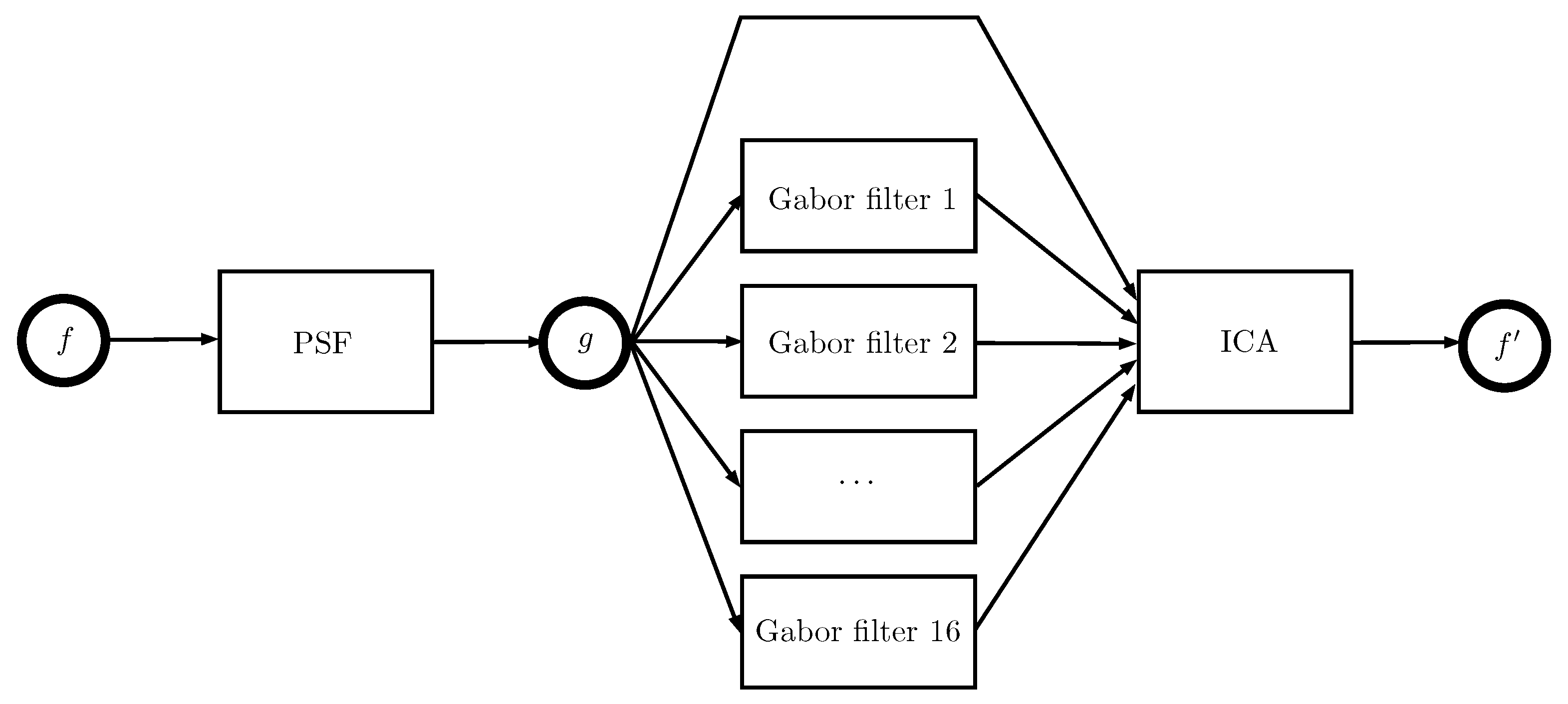
2.3. Blind Deblurring by Independent Component Analysis

Let us assume that the original image to recover is of size $n\times n$ and gray-level single channel, in such a way that the intensity function f may be represented as a $n\times n$ matrix. (Indeed, it is not essential for the image support to be square as all the relationships in this paper would hold for rectangular-support images as well.) In addition, let us assume that exactly the 16 Gabor filters described in Section 2.1 are used to construct pseudo-images to feed an ICA neural network. As a further working hypothesis, let us assume that convolution $\otimes$ does not alter the size of the original image, which entails little information loss as long as the size $2M+1$ of the PSF and the size $2G+1$ of the Gabor filter are much smaller than the size n of the image to process.

In order to build a data matrix to input an ICA neural network, the recorded image g and its 16 Gabor-filtered versions are vectorized into 17 arrays of size $n^2\times 1$, denoted by $g_i$, with $i=1,\dots ,17$. Such arrays are built by piling up pixel intensities scanned in lexicographic order. These arrays are then arranged into a data matrix X as follows:

$$X:=\left[\begin{array}{c}{g_1}^{\top }\\ {g_2}^{\top }\\ \cdots \\ {g_{17}}^{\top }\end{array}\right],$$

(8)

where the superscript ${}^{\top }$ denotes matrix transpose. The obtained data matrix therefore consists of 17 rows and $n^2$ columns.

As a pre-processing stage prior to performing independent component analysis, the data matrix needs to undergo three operations termed column-centering, row-shrinking and column-whitening, to be performed in this exact order.

• Column-centering consists of making the columns of the data matrix X zero-mean. Let us decompose the matrix X into its $n^2$ columns as follows:

  $$X=[x_1{x}_2{x}_3{x}_4\cdots x_{n^2}],$$

  (9)

  where each column-array $x_k$ has dimension $17\times 1$. The empirical mean value of the set of $n^2$ columns is calculated as

  $$m:=\frac{1}{n^2}\sum _{k=1}^{n^2}{x}_k,$$

  (10)

  and the centered columns of the data matrix are defined as

  $${\check{x}}_k:=x_k-m.$$

  (11)

  Let us denote by $\check{X}$ the matrix whose columns are ${\check{x}}_k$.
• Row-shrinking is based on empirical covariance estimation and on thresholding the eigenvalues of the estimated empirical covariance matrix [31]. The empirical covariance matrix associated to the columns of the centered data matrix $\check{X}$ is defined by:

  $$C_x:=\frac{1}{n^2}\sum _{k=1}^{n^2}{\check{x}}_k{\check{x}}_k^{\top }=\frac{1}{n^2}\check{X}{\check{X}}^{\top }.$$

  (12)

  and has dimensions $17\times 17$. The eigenvalue decomposition of the covariance matrix reads $C_x=ED{E}^{\top }$, where E is an orthogonal matrix of eigenvectors and D is a diagonal matrix of eigenvalues, namely $D=\mathrm{diag}(d_1,\dots ,d_{17})$, assumed to be ordered by decreasing values. Rank deficiency and numerical approximation errors might occur, which might make a number of eigenvalues in D be zero or even negative. Notice that, in particular, rank deficiency makes the matrix D be singular, which unavoidably harms the process of ‘whitening’, as explained in the next point. In order to mitigate such unwanted effect, it is customary to set a threshold (in this study, a value ${10}^{-4}$ was chosen as threshold) and to retain those ℓ eigenpairs corresponding to the ℓ eigenvalues above the threshold. The corresponding eigenmatrix pair is denoted by $(\tilde{E},\tilde{D})$, where $\tilde{E}$ is of size $\ell \times n^2$ and $\tilde{D}$ is of size $\ell \times \ell$. Since, most likely, $\ell <17$, thresholding has the effect of shrinking the centered data matrix.
• Column-whitening is a linear transformation applied to each column of the data matrix $\check{X}$ to obtain a quasi-whitened data matrix $Z=[z_1{z}_2{z}_3\cdots z_{n^2}]$ whose columns exhibit a unit covariance. Such linear transformation is described by

  $$Z={\tilde{D}}^{-1/2}{\tilde{E}}^{\top }\check{X}.$$

  (13)

  Notice that the whitened data matrix has size $\ell \times n^2$ and, in general, its covariance matrix is perfectly unitary only if row-shrinking did not take place, namely, only if $\ell =17$. If, however, some of the eigenvalues of the empirical covariance matrix $C_x$ are zero or negative, whitening is not possible since the (non-shrunken) matrix $D^{-1/2}$ is either not calculable or complex-valued.

The centered, shrunken and quasi-whitened data matrix Z is fed to an ICA neural network in order to extract the first independent component, namely, the one independent component $f^{\prime }$ that corresponds to the original sharp image f (up to an arbitrary—and inessential—scaling constant that may be compensated for while rendering the image). In the present instance, the ICA neural network is described by the linear input–output transformation:

$$p:=w^{\top }Z,$$

(14)

where w denotes a real-valued array of size $\ell \times 1$ of weights termed weight vector. The array p has size $1\times n^2$. The weight vector, which is subjected to an information-based learning process, is adapted according to a two-stage non-linear learning rule [11]. The first stage is described by:

$$w\leftarrow w+\mu Z{tanh}^{\top }(p),$$

(15)

where $\mu >0$ denotes a learning step size and the function ‘tanh’ denotes a hyperbolic tangent function that acts component-wise on the array p and represents an activation function for the single-neuron ICA-type artificial neural system. The second stage is described by a projection rule:

$$w\leftarrow \frac{w}{\parallel w\parallel },$$

(16)

which normalizes the weight vector to the unit hypersphere and prevents the weight vector to either drop to zero or to diverge. The two stages are repeated until the weight vector reaches a stable configuration, which corresponds to a learned neural network. Given the structure of the above learning procedure, it is referred to in the following as the update-and-project learning rule.

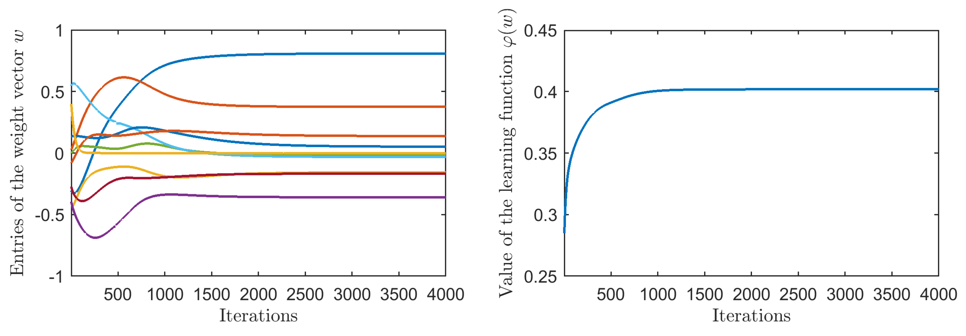
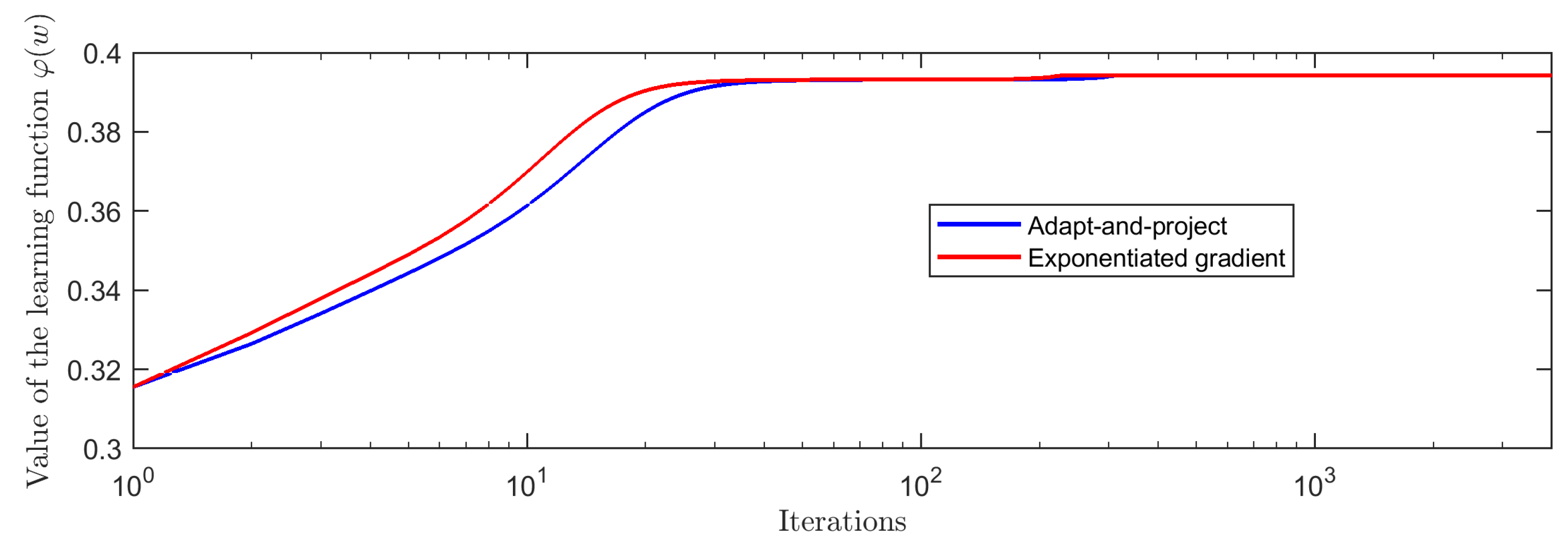
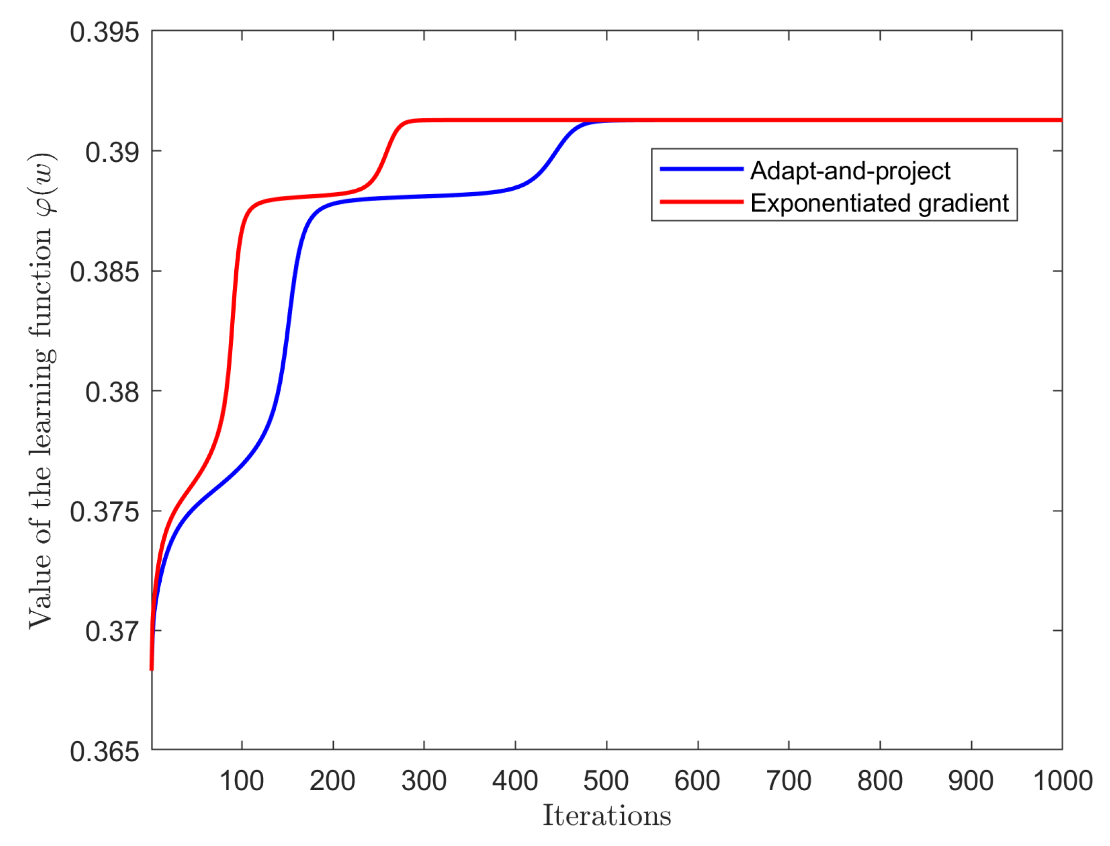
2.4. An ICA Learning Algorithm Based on Exponentiated Gradient on the Unit Hypersphere

Since the neural weight vector w is to be sought under the compelling constraint of unit norm, independent component learning may first be formulated as an optimization problem on the unit hypersphere. Such optimization problem may be solved by an exponentiated Riemannian gradient numerical algorithm on the unit hypersphere, as outlined below.

The real ℓ-dimensional unit hyper-sphere [32] is a smooth manifold defined as

$${𝕊}^{\ell -1}:=\{w\in {ℝ}^{\ell }|w^{\top }w=1\}.$$

(17)

On the basis of manifold calculus particularized to the unit hypersphere, the weight vector w that extracts the first independent component from the data matrix Z may be learned by an alternative algorithm to the two-stage method in (15) and (16). The key concept is to formulate the ICA problem as the search for the maximum of a smooth function and to employ a numerical exponentiated-gradient-based optimization algorithm to solve such maximization problem.

To this aim, let us recall the notion of exponential map $exp:T{\mathbb{S}}^{\ell -1}\to {\mathbb{S}}^{\ell -1}$ (where $T{\mathbb{S}}^{\ell -1}$ denotes the tangent bundle associated to the unit hypersphere), associated to the canonical metric, defined by

$${exp}_x(v):=\left\{\begin{array}{cc}xcos(\parallel v\parallel )+\frac{vsin(\parallel v\parallel )}{\parallel v\parallel }\hfill & \mathrm{if} v\ne 0,\hfill \\ x\hfill & \mathrm{otherwise},\hfill \end{array}\right.$$

(18)

where $x\in {\mathbb{S}}^{\ell -1}$, $v\in T_x{\mathbb{S}}^{\ell -1}$ and the symbol $\parallel ·\parallel$ denotes standard vector 2-norm. Let us also recall the expression of the Riemannian gradient of a smooth function $\phi :{\mathbb{S}}^{\ell -1}\to \mathbb{R}$ associated to the canonical metric:

$${\nabla }_x\phi :=\left(I_{\ell }-x{x}^{\top }\right)\frac{\partial \phi }{\partial x},$$

(19)

where $\frac{\partial \phi }{\partial x}$ denotes the Euclidean gradient at x and $I_{\ell }$ denotes an identity matrix of size $\ell \times \ell$.

On the basis of the definitions (18) and (19), an exponentiated gradient algorithm to seek for the maximum point of the function $\phi$ may be expressed as:

$$w\leftarrow {exp}_w(\mu {\nabla }_w\phi ),$$

(20)

where, by definition of exponential map,

$${exp}_w(\mu {\nabla }_w\phi )=wcos(\parallel \mu {\nabla }_w\phi \parallel )+\frac{sin(\parallel \mu {\nabla }_w\phi \parallel ){\nabla }_w\phi }{\parallel {\nabla }_w\phi \parallel },$$

(21)

hence the updating rule may be written as the one-step assignment

$$w\leftarrow wcos(\parallel \mu {\nabla }_w\phi \parallel )+\frac{sin(\parallel \mu {\nabla }_w\phi \parallel ){\nabla }_w\phi }{\parallel {\nabla }_w\phi \parallel }.$$

(22)

The constant $\mu >0$ denotes again a learning step size to be chosen beforehand.

The function $\phi$ whose maximum is sought may be related to the ICA problem according to the following reasoning. A non-linear function of the weight vector that is a valid criterion to achieve one-component ICA reads [30]:

$${\mathcal{E}}_z\left[A(w^{\top }z)\right]:={\int }_{{\mathbb{R}}^{\ell }}A(w^{\top }z){\rho }_z(z)d{z}^{\ell },$$

(23)

where $A:\mathbb{R}\to \mathbb{R}$ denotes a non-linear function and ${\rho }_z:{\mathbb{R}}^{\ell }\to {\mathbb{R}}_0^{+}$ denotes the joint probability density function of the ℓ observations that input the neural network (that the columns of the data matrix Z constitute realizations of). The symbol ${\mathcal{E}}_z[·]$ denotes statistical expectation. The integral, which may seldom be evaluated exactly, may be approximated by a finite sum, hence the criterion function $\phi$ that arises from the above principle may be defined as:

$$\phi (w):=\sum _{k=1}^{n^2}A(w^{\top }{z}_k)\mathrm{Pr}(z_k)\Delta z^{\ell },$$

(24)

in which $\mathrm{Pr}(z_k)\in [0,1]$ denotes the probability associated to the sample $z_k$ and the expression $\Delta z^{\ell }$ denotes the volume of a tiny hypercube centered around the sample $z_k$. The Euclidean gradient of the function $\phi$ with respect to its vector-type argument w reads:

$$\frac{\partial \phi }{\partial w}=\sum _{k=1}^{n^2}{A}^{\prime }(w^{\top }{z}_k)z_k\mathrm{Pr}(z_k)\Delta z^{\ell }.$$

(25)

Taking $A:=ln\circ cosh$ leads to $A^{\prime }=tanh$. Such choice for the discriminant non-linearity is not compelling although is supposed to loosely match the statistical distribution of the source components [30]. For simplicity, the statistical distribution of the samples $z_k$ may be assumed uniform, namely $\mathrm{Pr}(z_k)=\frac{1}{n^2}$, therefore:

$$\frac{\partial \phi }{\partial w}=\frac{\Delta z^{\ell }}{n^2}\sum _{k=1}^{n^2}tanh(w^{\top }{z}_k)z_k=\frac{\Delta z^{\ell }}{n^2}Ztanh(Z^{\top }w),$$

(26)

where the hyperbolic tangent function is assumed to act component-wise on a vector-type argument. Recalling the definition (14), one may write

$$\frac{\partial \phi }{\partial w}=\frac{\Delta z^{\ell }}{n^2}Z{tanh}^{\top }(p),$$

(27)

where p denotes again the response of the ICA neural network as defined in (14). Since the volume element $\Delta z^{\ell }$ is constant, it may be absorbed in the learning rate and may thus be safely set to 1. Conversely, the coefficient inversely proportional to $n^2$ is retained to scale the sum that grows with the size of the image under processing. Therefore, according to the general formula (19), the Riemannian gradient of the function $\phi$ reads:

$${\nabla }_w\phi =\frac{1}{n^2}\left(I-w{w}^{\top }\right)Z{tanh}^{\top }(p)=\frac{1}{n^2}\left(Z-wp\right){tanh}^{\top }(p)$$

(28)

In conclusion, the proposed exponentiated-gradient learning rule for the ICA neural network reads:

$$\left\{\begin{array}{c}{\nabla }_w\phi =\frac{1}{n^2}\left(Z-wp\right){tanh}^{\top }(p),\hfill \\ w\leftarrow wcos(\parallel \mu {\nabla }_w\phi \parallel )+\frac{{\nabla }_w\phi sin(\parallel \mu {\nabla }_w\phi \parallel )}{\parallel {\nabla }_w\phi \parallel }.\hfill \end{array}\right.$$

(29)

The exponentiated-gradient learning sweep of the data matrix is repeated until the weight vector reaches a stable configuration. Progress of learning may be monitored by checking either the components of the weight vector or the value of the criterion function.

In order to check whether the neural ICA algorithm has reached a stable configuration of the weights, it is worth monitoring the values of the weights as well as the value taken by the criterion function $\phi$. The absolute value of the index $\phi$ is not meaningful, since it depends on the input statistics, but its time-course has meaning, since it tells how effective a learning session has been.

3. Experimental Results

The present section discusses a number of experimental results obtained on test images, where the blur is obtained by a known PSF, as well as on real-world images, which were acquired through a defocused lens. The process of deblurring is carried out by the adapt-and-project algorithm (on occasions abbreviated as AAP) recalled in Section 2.3 as well as by the exponentiated-gradient method (occasionally abbreviated as EG) explained in Section 2.4. Cases of successful deblurring are presented and cases of unsuccessful deblurring are discussed through a comprehensive set of experiments.

3.1. Experiments on Deblurring Artificially Blurred Images

In the first numerical experiment, a sharp gray-scale image, with $n=240$ pixels per row/column, was artificially blurred by means of Gaussian point-spread functions of different sizes:

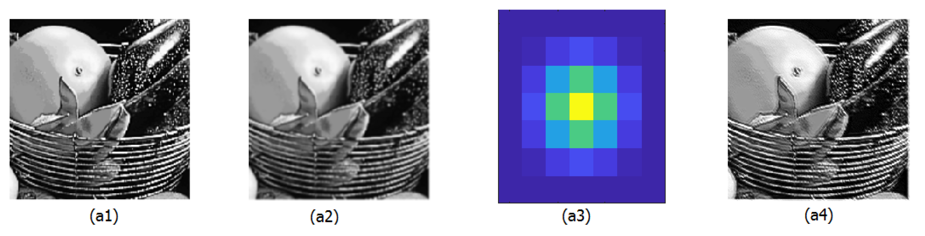
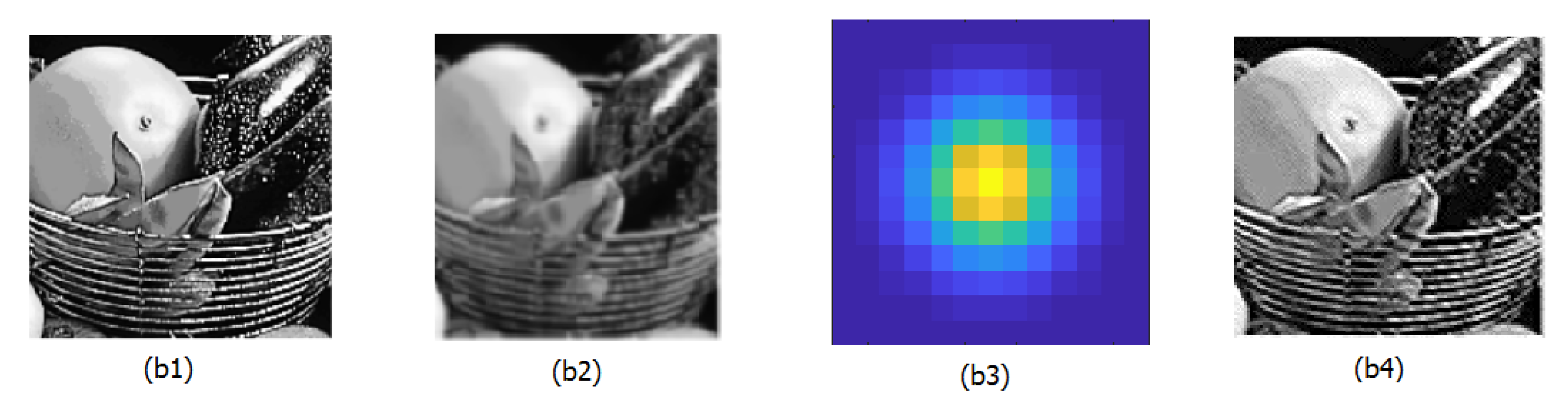
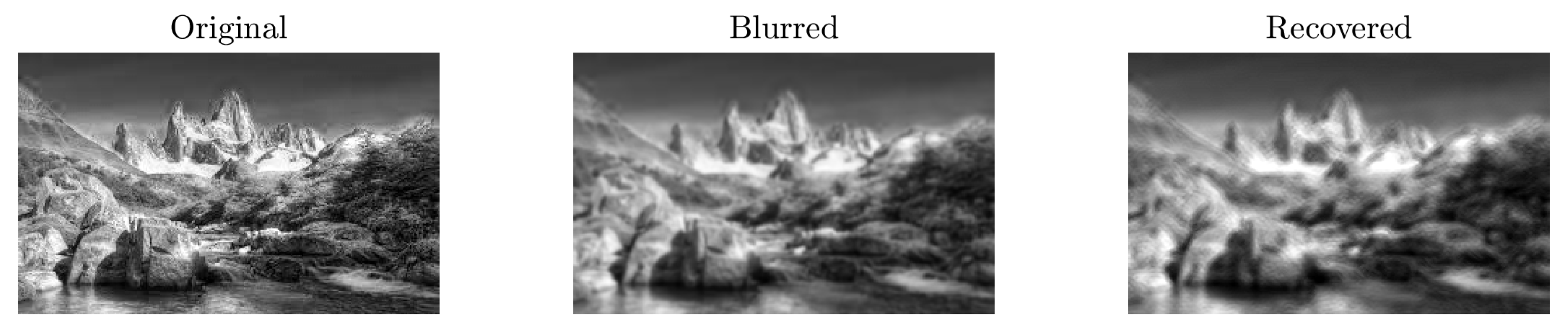
• An isotropic point-spread function with variance 1, denoted as Gaussian-(1,1): The clean image, the blurred image and the point-spread function are shown in Figure 4. In this case, the PSF has size $M=3$.
• An isotropic point-spread function with variance 2, denoted as Gaussian-(2,2): The clean image, the blurred image and the point-spread function are shown in Figure 5. In this case, the PSF has size $M=6$.

In blind deblurring, it is indeed customary to assume that the PSF is described by a Gaussian kernel [33].

The Gabor filters used in these experiments are the ones explained in Section 2.1 with filter size $G=4$. Upon applying centering and row-shrinking of the data matrix, $\ell =10$ rows of the data matrix were retained out of 17. The shrinking sub-procedure proved, therefore, necessary to achieve a quasi-whitened data matrix. The learning rate for the neural ICA algorithms discussed in Section 2.3 and Section 2.4 was set to $\mu ={10}^{-5}$. The results of the exponentiated-gradient neural ICA-based deblurring algorithm are illustrated in the rightmost panels of Figure 4 and Figure 5.

Figure 6 shows the evolution of the ℓ components of the weight vector w during learning. The total number of iterations was set to 4000, although the convergence of the weight vector is achieved after nearly 2000 iterations. After that, the weight values change only slightly, confirming that the learning process has reached a stable configuration and that the algorithmic implementation is numerically stable. Figure 6 also shows the values of the learning criterion $\phi$ during iterations. The shape of such curve confirms that the ICA neural network gets trained by seeking for the maximum value of the criterion function.

To compare the original adapt-and-project neural ICA method to the proposed exponentiated-gradient method, the coefficient of correlation between the original image and the blurred image, as well as between the original image and the deblurred image, as recovered by both algorithms, were calculated, as shown in

Table 1. Comparison of the original adapt-and-project (AAP) neural ICA method to the proposed exponentiated-gradient (EG) method: Coefficients of correlation between the original image and the blurred image and between the original image and the deblurred image.

PSF	Original/Blurred	Original/Deblurred (AAP)	Original/Deblurred (EG)
Gau-(1,1)	0.9658	0.9682	0.9684
Gau-(2,2)	0.8836	0.9484	0.9509

.

The results summarized in Table 1 show that the Gaussian-(2,2) point-spread function causes a more severe blur. The Gaussian-(1,1) point-spread function causes a slight blur that was mitigated equally successfully by both neural learning methods. Both methods achieve restoration of the original image, as the correlation coefficient between the original and the restored image is higher than the correlation coefficient between the original and the blurred image. The level of restoration achieved by the exponentiated-gradient method is larger than the level of restoration achieved by the adapt-and-project method.

As a further element of comparison, the learning curves of both neural methods were traced out in the same panel to compare their convergence speed when $\mu ={10}^{-6}$. Figure 7 shows that the exponentiated-gradient method converges more quickly than the adapt-and-project method. As illustrated in the next subsection, by increasing the learning step size, the separation between the two curves increases and the EG learning algorithm may be shown to converge more quickly than the AAP learning algorithm while retaining numerical stability and independent component extraction ability.

3.2. Limitations of the Restoration Method on Artificially Blurred Images

Image deblurring based on Gabor filtering and first independent component analysis is not universal and cannot be expected to be able to effectively deblur any sort of images. The limitations of such method are not only due to the learning rule that the ICA network is trained by, but also on the fact that the first independent component extracted from a data matrix does not necessarily coincide with the f-component in the Taylor expansion (6).

It is quite apparent from the experiments how images containing fine details cannot be recovered from their blurred observations, as can be seen, for instance, in Figure 8. Such result was obtained by a $533\times 800$ image blurred by a Gaussian-(2,2) point-spread function. The number of retained data matrix rows after shrinking was $\ell =10$. An explanation of this malfunctioning is that the first independent component extracted by the neural network from the linear mixing explained by the model (6) is a superposition of the original image f and of its (higher-frequency) spatial derivatives.

In addition, it is quite apparent that low-resolution natural images cannot be recovered from their blurred recordings, as can be seen from the result illustrated in Figure 9. Such result was obtained on a $177\times 284$ image blurred by a Gaussian-(1,1) point-spread function. Even in this experiment, the number of retained data matrix rows after shrinking was $\ell =10$. Although the neural ICA network reaches a stable configuration of the weights, hence learns to perform the ICA task, the first independent component extracted by the neural network does not coincide to a good approximation with the original image f, possibly because of the lack of enough statistical information due to a limited number of pixels in the image.

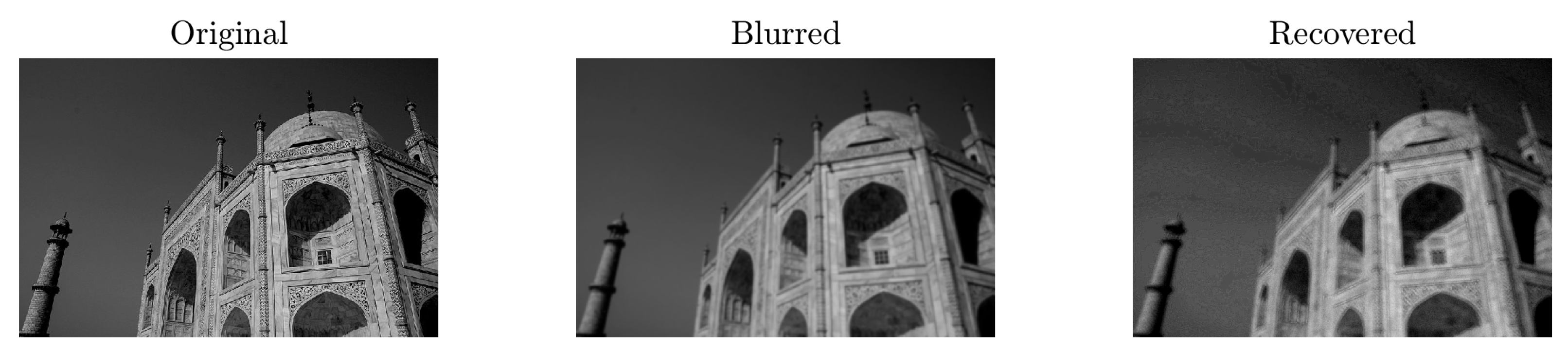
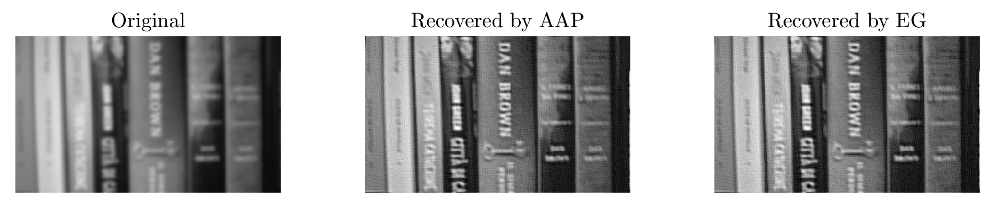
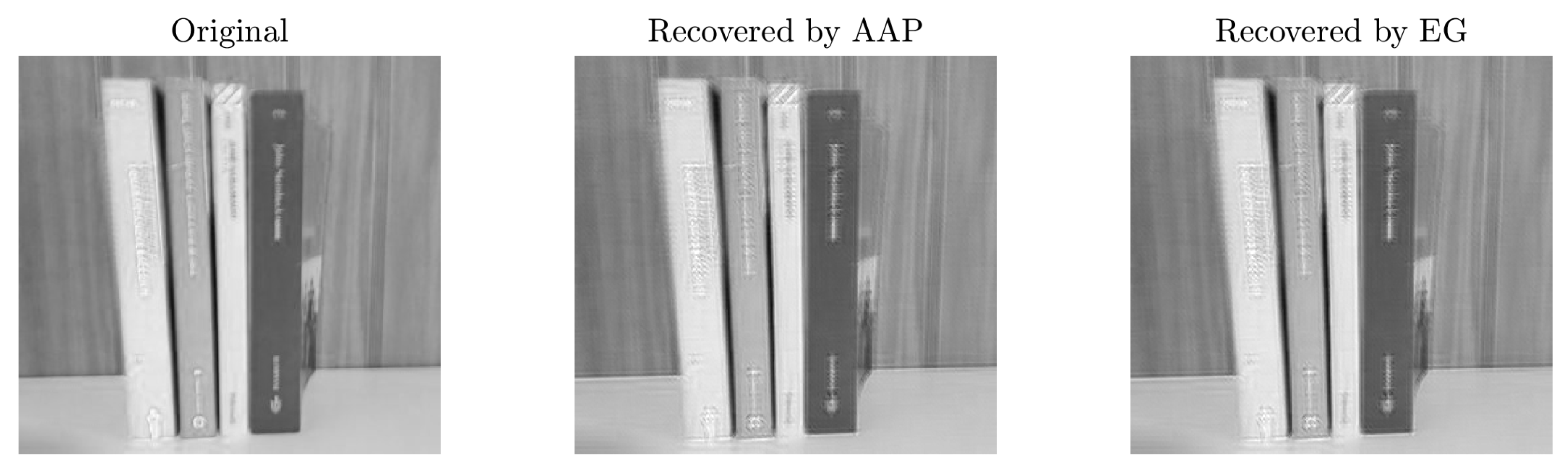
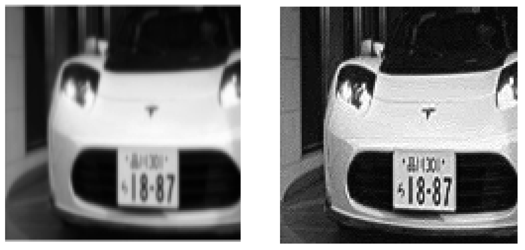
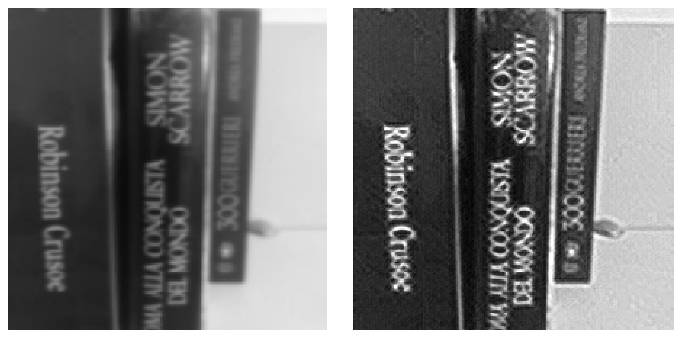
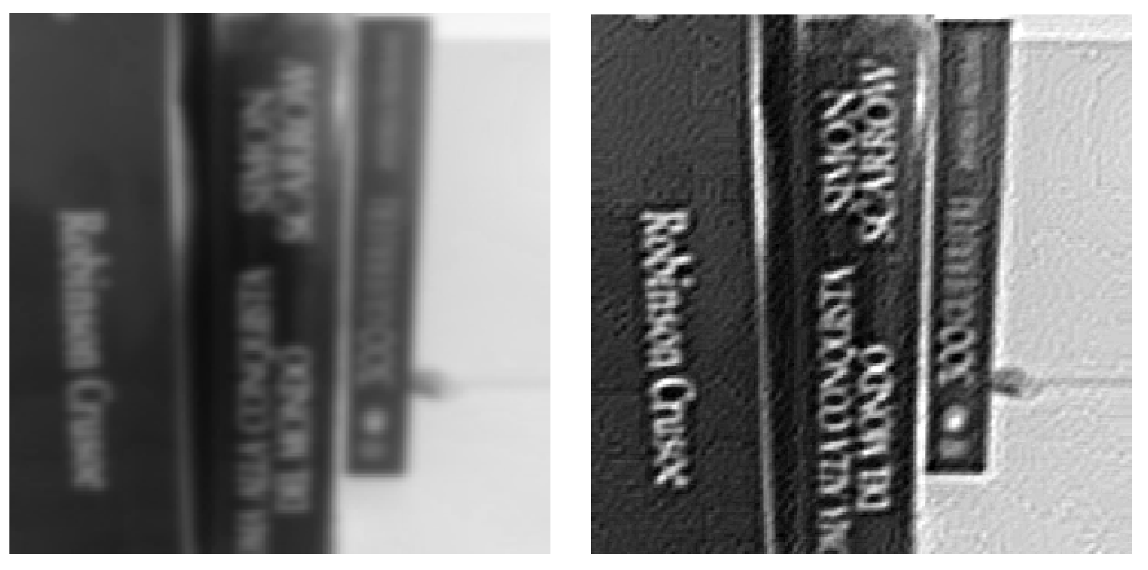
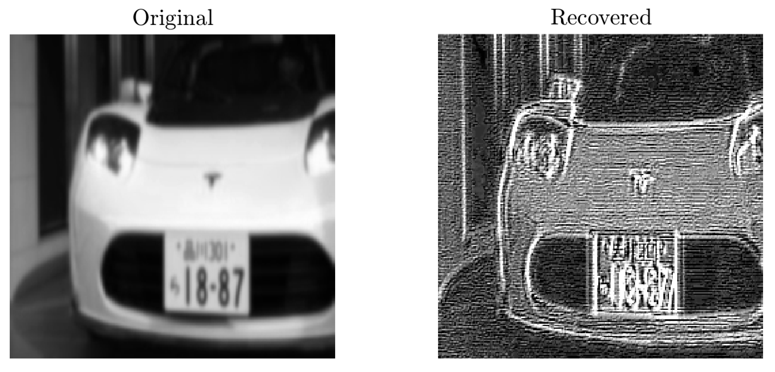
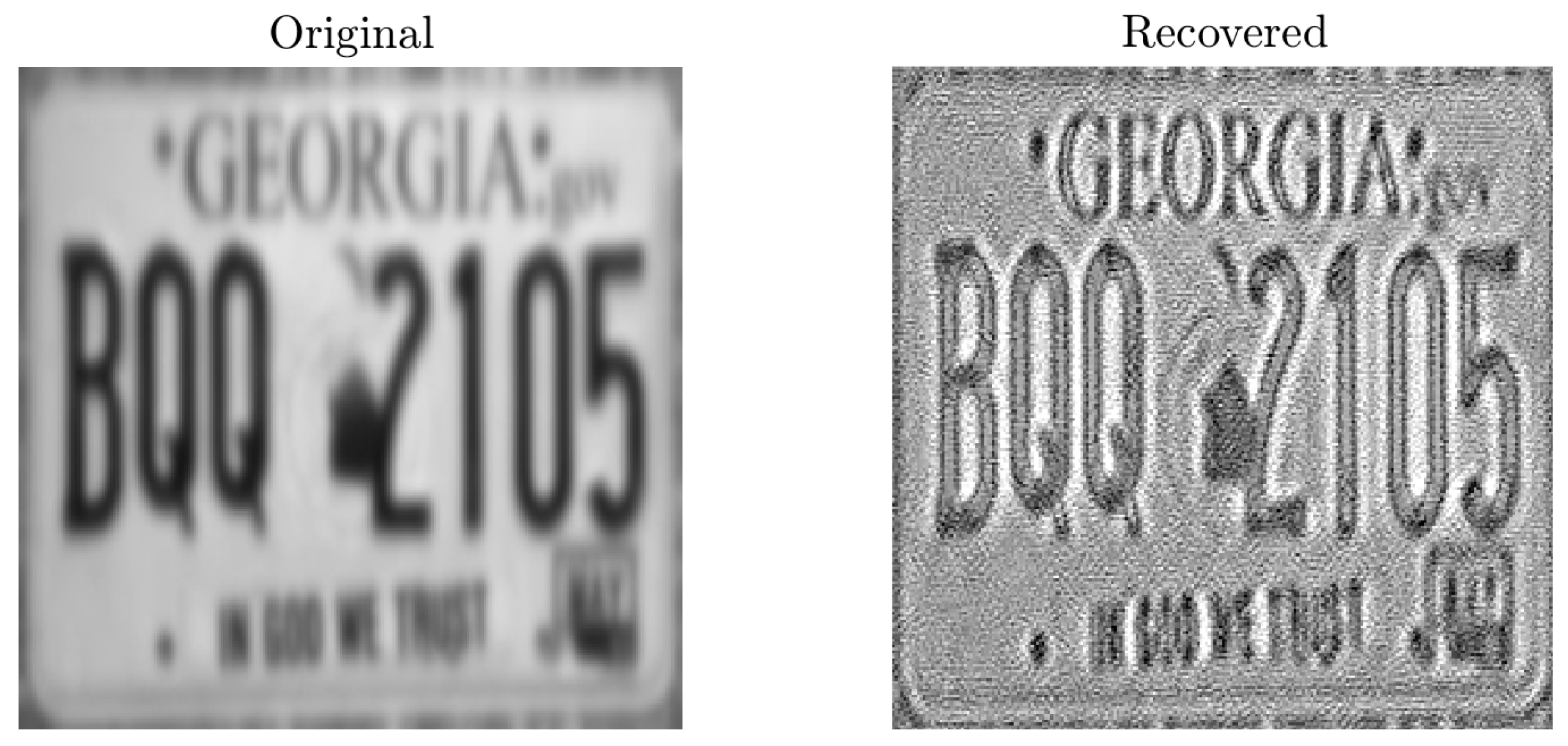
3.3. Experiments on Deblurring Naturally Blurred Images

The adapt-and-project method and the exponentiated-gradient method were applied to re-focusing a naturally blurred image. In particular, the image shown in the left-hand panel of Figure 10 was recorded frontally by a digital camera through an out-of-focus lens. Such blurred image, of size $187\times 317$, was filtered by 16 Gabor filters and the result was subjected to centering, shrinking ($\ell =10$) and whitening. The result of deblurring by first independent component analysis by the two neural learning methods is shown in the middle panel and in the right-hand panel of Figure 10. The words on the back of the books are more easily readable in the recovered images.

It is important to underline again that the discussed deblurring method is based on the hypothesis that the point-spread function keeps constant across the image support. This is not always true: when an image is recorded non-frontally (i.e., slanted), different objects in the image are defocused in different ways. Figure 11 shows an image taken non-frontally through an out-of-focus lens. The image has size $302\times 320$. Despite the good resolution of the recorded image and of the relatively marginal presence of fine details, the result of deblurring does not appear as good as that shown in Figure 10.

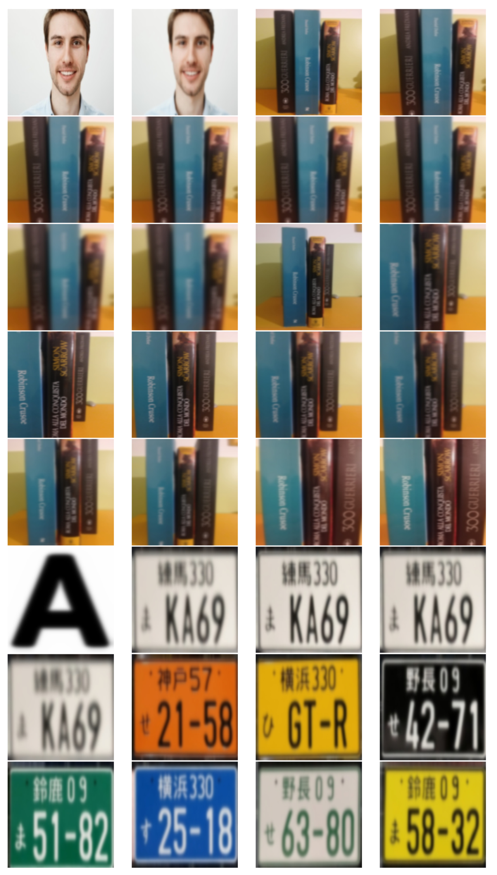
3.4. First Comprehensive Set of Experiments

On the basis of the preliminary experiments discussed in the previous subsections, which evidenced how the recalled/extended blind image deblurring method is effectively capable of improving the quality of a blurred image, while it cannot under particular circumstances, we proceeded with a number of experiments on real-world images.

The images used in the present set of experiments exhibit different levels of defocusing expressed through a percentage. Moreover, most images are in Portable Network Graphics (.png) format with a resolution of $240\times 240$ pixels. In total, 33 images were used in the present comprehensive test. Each image differs from the others by type (file format, resolution and distance between two subjects on the same image) or subject (books, plate tags, cars and text). The first 32 test images are shown in Figure 12.

Table 2. Deblurring results on a set of 33 test images included in the first comprehensive set of experiments.

Image	Subject	Blur Type	Result
01_IM	Male face	10% defocusing	D
02_IM	Male face	30% defocusing	D
03_IM	Books on background	10% defocusing, 40 cm away	D
04_IM	Books on background	20% defocusing, 20 cm away	A
05_IM	Books on background	30% defocusing, 20 cm away	C
06_IM	Books on background	37.5% defocusing	B
07_IM	Books on background	37.5% defocusing, 300 × 300 pixels	C
08_IM	Books on background	37.5% defocusing, 200 × 200 pixels	C
09_IM	Books on background	50% defocusing, 20 cm away	D
10_IM	Books staggered of 10 cm	10% defocusing, 40 cm away	D
11_IM	Books staggered of 10 cm	40% defocusing, 10 cm away	C
12_IM	Books staggered of 10 cm	10% defocusing, 10 cm away	B
13_IM	Books staggered of 7 cm	10% defocusing, 10 cm away	A
14_IM	Books staggered of 7 cm	25% defocusing, 10 cm away	A
15_IM	Books staggered of 7 cm	30% defocusing, 10 cm away	C
16_IM	Books staggered of 5 cm	30% defocusing, 10 cm away	C
17_IM	Lined-up books	30% defocusing, 20 cm away	C
18_IM	Lined-up books	30% defocusing, 10 cm away	D
19_IM	Lined-up books	20% defocusing, 10 cm away	D
20_IM	Giant letter	100% defocusing	A
21_IM	White tag	100% defocusing	D
22_IM	White tag	60% defocusing	A
23_IM	White tag	70% defocusing	B
24_IM	White tag	80% defocusing	D
25_IM	Orange tag	60% defocusing	B
26_IM	Yellow tag	60% defocusing	B
27_IM	Black tag	60% defocusing	D
28_IM	Green-white tag	60% defocusing	D
29_IM	Blue tag	60% defocusing	D
30_IM	White-green tag	60% defocusing	A
31_IM	Canary yellow tag	60% defocusing	A
32_IM	Red-white tag	60% defocusing	D
33_IM	Car with passenger	20% defocusing	A

shows a summary of the results obtained on each of these 33 images. The outcome of each test was evaluated by one of four grades: (A) the image was well recovered; (B) the appearance of the image is noticeably better than the original one; (C) the image results to be slightly better than the original one; and (D) the image was not deblurred at all or was spoiled by the algorithm. In general, a dark foreground contrasting with a light background favor the focusing of plate tag images.

The results summarized in Table 2 are suggestive of a series of guidelines about the usage of the deblurring method, as discussed below:

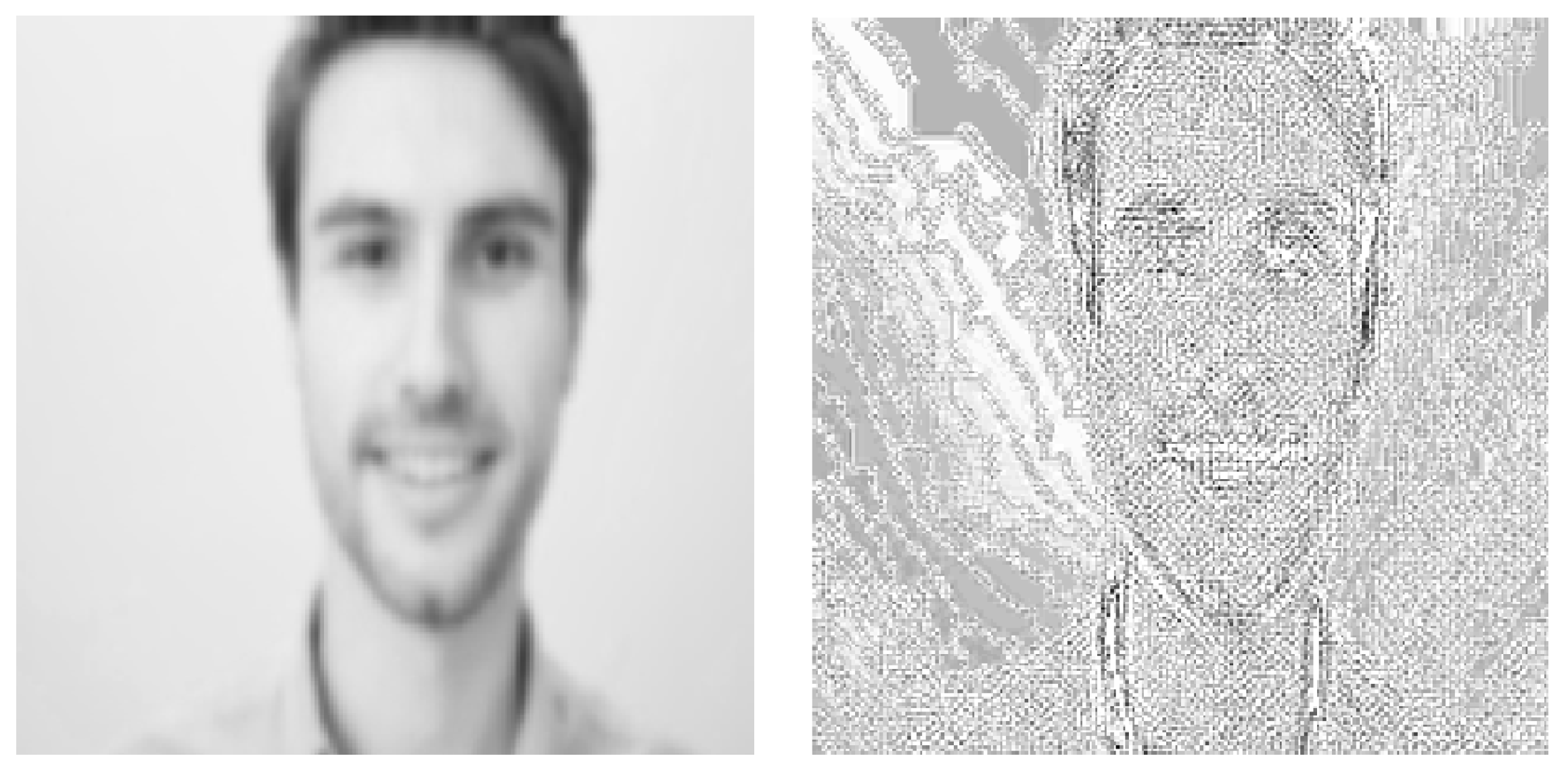
• In general, the discussed deblurring method performed poorly on human faces, unless the level of blur was moderate.
• When a picture originated from a phone camera, the distance between the subject and the camera should range between 10 and 30 cm to achieve a good result (over 40 cm of distance, deblurring was not achieved successfully).
• Distance and defocusing level should be inversely proportional to one another: the farther the subject, the lower the defocusing level should be.
• In general, the level of defocusing should range between 1% and 40% to achieve a B or A result; however, there are exceptions. In fact, an excellent result was obtained on a 100% defocused large-sized text.
• Although most images were of size 240 pixels × 240 pixels, comparable results were obtained on images whose size ranged between 200 × 200 and 300 × 300 pixels.
• The file format (image encoding algorithm) did not seem to influence the final result.
• In general, objects in the foreground resulted to be more focused than objects in the background; according to our estimations, good results were achieved up to 7 cm of staggering with a maximum initial defocusing of 30%.

Pictorial instances of the results summarized in Table 2 are displayed in the following figures.

Figure 13 clearly illustrates an A-scored result. The deblurring algorithm returns a clear image of the car, in which it is even possible to spot the silhouette of two occupants.

Figure 14 shows the result of deblurring on an input image that resulted to be slightly defocused. The ICA-based deblurring algorithm, in this instance, worked fine, since the books in the foreground are well-focused. The same cannot be said about the book in the background, thus this result scored a B grade.

The result illustrated in Figure 15 refers to the same input image as for the previous test (namely, the image shown in Figure 14), but more severely defocused. In this experiment, not only the text in the background but even that in the foreground look still out of focus after processing. For this reason, the outcome of this experiment was scored a C grade.

Figure 16 clearly illustrates a D-scored result. In this instance, the deblurring algorithm returns a distorted image of a human face.

3.5. Second Comprehensive Set of Experiments

A further series of comprehensive experiments was conducted on a data set of 29 license plate images, 28 of which are shown in Figure 17. In such dataset, therefore, all pictures concern the same subject.

A purpose of the present group of experiments was to train an ICA neural network with a sequence of images. At the beginning of the training phase, the weight vector of the ICA network was instantiated randomly over the unit hypersphere, while each subsequent learning cycle started from the weight vector configuration learned during the previous adaptation cycle. Each learning cycle consisted of 4000 presentations of the same image as input to the neural system. The result of such test is displayed in Figure 18.

As the displayed curves suggest, each time a new image is presented, the learning cycle starts over and a new stable configuration is reached, which, in general, looks quite different from the previous one. Such result evidences that the ICA learning process trained sequentially is unable to fuse the information from several sources and that a globally optimal solution to the deblurring problem does not seem to exist. Rather, deblurring each image appears as a separate problem whose solution needs to be learned from scratch. In other terms, an ICA neural system with a single unit seems unable to generalize while trained sequentially. Interestingly, with the only noticeable exceptions corresponding to the Images 10 and 23, the values learned in correspondence of the other 27 images lie approximately in the same intervals. For the benefit of the reader, a red frame marks Images 10 and 23 in Figure 17. Image 23 certainly differs from the other images in the same training set, which justifies a markedly different deblurring filter learned.

To further confirm the above interpretation of the results displayed in Figure 18 by learning curves, it is instructive to feed a learned ICA network: (a) an image that did not belong the training set; and (b) an image that did belong to the training set (but that differ from the last image presented during the learning phase). Figure 19 shows a result for Case (a), As can be verified directly, the resulting output of the ICA neural system is neither clear nor very blurred. Figure 20 shows a result for Case (b). Again, the output of the ICA neural system is neither clear nor very blurred.

The obtained results are indeed dependent on the order of presentation of the single images; in fact, a different order produces different outcomes for the same experiments. The result of deblurring an image that did not belong to the training set is illustrated in Figure 21, while the result of deblurring an image that did belong to the training set is illustrated in Figure 22. Although the visual results look somewhat appreciable, the learned refocusing filter w was clearly learned from the ICA neural system to deblur a different kind of image.

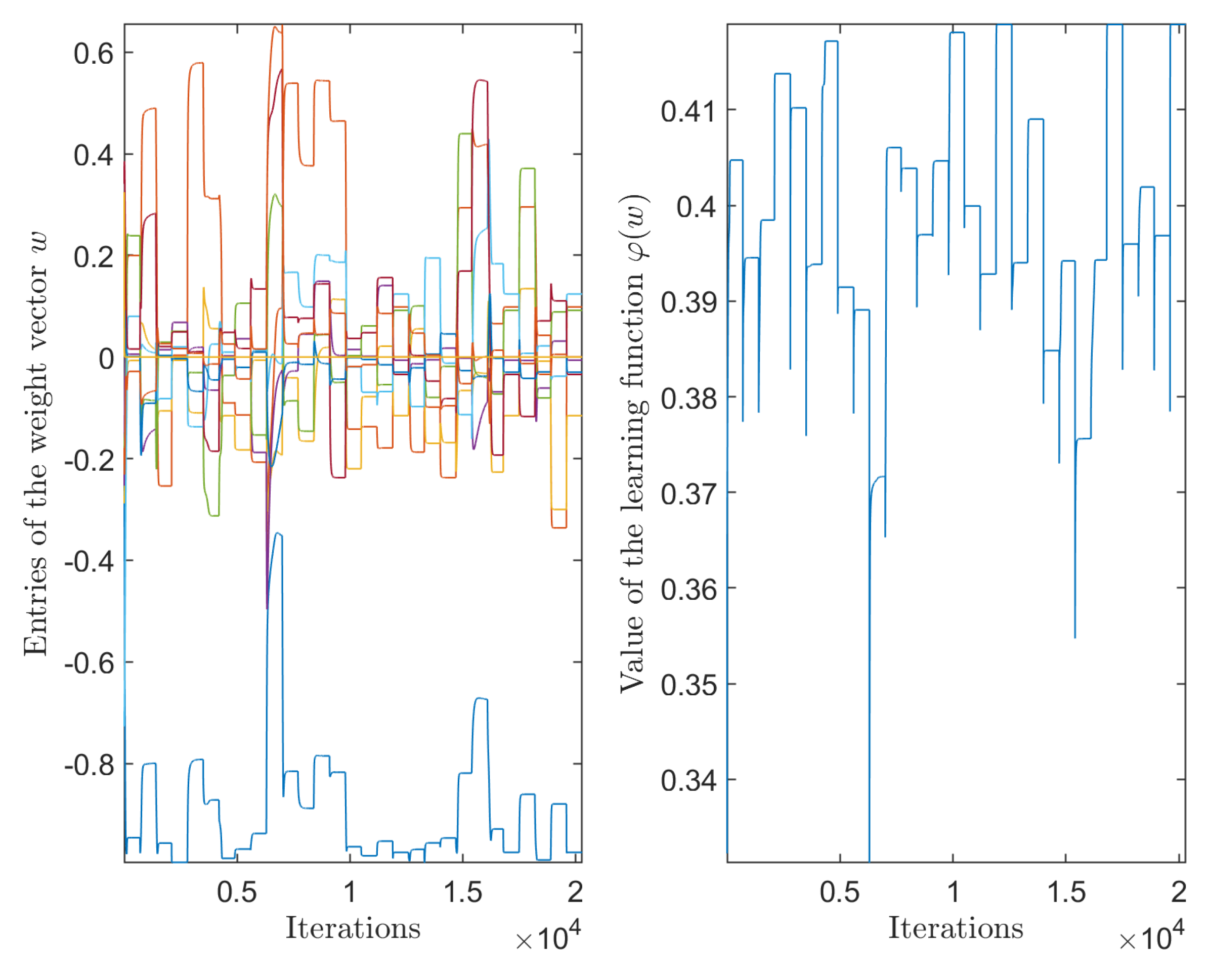
3.6. Experiments on Choosing a Suitable Learning Step Size

Conventional learning algorithms heavily rely on a correct choice of a sufficiently small value of the learning step size ($\mu$) to warrant numerical stability, yet sufficiently large to ensure reasonably fast convergence. Manifold calculus-based algorithms rely less on such trade-off because, for compact manifolds such as the unit hypersphere, numerical stability is an inherent property of the learning algorithm; hence, in general, larger step sizes may be selected and faster convergence may be expected.

The above statement is substantiated by a comparison of learning curves obtained on the image shown in Figure 23.

The result of comparison is shown in Figure 24. The net result is that the EG-based ICA learning algorithm may converge more quickly that the AAP-based learning algorithm.

4. Conclusions

The aim of this study was to recall a method to achieve blind image deblurring based on a clever application of the independent component analysis technique and to compare the originally utilized adapt-and-project first independent component learning method to a novel exponentiated-gradient learning method. Both methods are based on a convolutional model of the blurred image and a pre-filtering of the blurred image by a set of Gabor filters. The discussed methods are potentially able to recover the clean image without knowing (or estimating) the point-spread function.

Several numerical experimental results are presented and discussed to evidence objectively the good features of the method as well as its deficiencies and compare the adapt-and-project first independent component learning algorithm to the exponentiated-gradient learning algorithm. In particular, the experiments evidenced how the novel exponentiated-gradient learning method converges more quickly than the adapt-and-project first independent component learning algorithm and is able to extract an image that is more coherent to the clean image than the original algorithm.

References

1. Lai, W.; Huang, J.; Hu, Z.; Ahuja, N.; Yang, M. A Comparative Study for Single Image Blind Deblurring. In Proceedings of the 2016 IEEE Conference on Computer Vision and Pattern Recognition (CVPR), Las Vegas, NV, USA, 26 June–1 July 2016; pp. 1701–1709. [Google Scholar] [CrossRef]
2. Bahat, Y.; Efrat, N.; Irani, M. Non-uniform Blind Deblurring by Reblurring. In Proceedings of the 2017 IEEE International Conference on Computer Vision (ICCV), Venice, Italy, 22–29 October 2017; pp. 3306–3314. [Google Scholar] [CrossRef]
3. Zhang, H.; Wipf, D.; Zhang, Y. Multi-image Blind Deblurring Using a Coupled Adaptive Sparse Prior. In Proceedings of the 2013 IEEE Conference on Computer Vision and Pattern Recognition, Portland, OR, USA, 23–28 June 2013; pp. 1051–1058. [Google Scholar] [CrossRef]
4. Srinivasan, P.P.; Ng, R.; Ramamoorthi, R. Light Field Blind Motion Deblurring. In Proceedings of the 2017 IEEE Conference on Computer Vision and Pattern Recognition (CVPR), Honolulu, HI, USA, 21–26 July 2017; pp. 2354–2362. [Google Scholar] [CrossRef] [Green Version]
5. Fiori, S. Fast fixed-point neural blind-deconvolution algorithm. IEEE Trans. Neural Netw. 2004, 15, 455–459. [Google Scholar] [CrossRef]
6. Levin, A.; Weiss, Y.; Durand, F.; Freeman, W.T. Understanding Blind Deconvolution Algorithms. IEEE Trans. Pattern Anal. Mach. Intell. 2011, 33, 2354–2367. [Google Scholar] [CrossRef]
7. Vorontsov, S.V.; Jefferies, S.M. A new approach to blind deconvolution of astronomical images. Inverse Probl. 2017, 33, 055004. [Google Scholar] [CrossRef]
8. Brylka, R.; Schwanecke, U.; Bierwirth, B. Camera Based Barcode Localization and Decoding in Real-World Applications. In Proceedings of the 2020 International Conference on Omni-layer Intelligent Systems (COINS), Barcelona, Spain, 31 August–2 September 2020; pp. 1–8. [Google Scholar] [CrossRef]
9. Lou, Y.; Esser, E.; Zhao, H.; Xin, J. Partially Blind Deblurring of Barcode from Out-of-Focus Blur. SIAM J. Imaging Sci. 2014, 7, 740–760. [Google Scholar] [CrossRef] [Green Version]
10. Umeyama, S. Blind deconvolution of blurred images by use of ICA. Electron. Commun. Jpn. (Part III Fundam. Electron. Sci.) 2001, 84, 1–9. [Google Scholar] [CrossRef]
11. Umeyama, S. Blind deconvolution of images using Gabor filters and independent component analysis. In Proceedings of the 4th International Symposium on Independent Component Analysis and Blind Signal Separation, Nara, Japan, 1–4 April 2003; pp. 319–324. [Google Scholar]
12. Lei, S.; Zhang, B.; Wang, Y.; Dong, B.; Li, X.; Xiao, F. Object Recognition Using Non-Negative Matrix Factorization with Sparseness Constraint and Neural Network. Information 2019, 10, 37. [Google Scholar] [CrossRef] [Green Version]
13. Wu, Y.; Wang, X.; Zhang, T. Crime Scene Shoeprint Retrieval Using Hybrid Features and Neighboring Images. Information 2019, 10, 45. [Google Scholar] [CrossRef] [Green Version]
14. Aladjem, M.; Israeli-Ran, I.; Bortman, M. Sequential Independent Component Analysis Density Estimation. IEEE Trans. Neural Netw. Learn. Syst. 2018, 29, 5084–5097. [Google Scholar] [CrossRef] [PubMed]
15. Cai, L.; Tian, X.; Chen, S. Monitoring Nonlinear and Non-Gaussian Processes Using Gaussian Mixture Model-Based Weighted Kernel Independent Component Analysis. IEEE Trans. Neural Netw. Learn. Syst. 2017, 28, 122–135. [Google Scholar] [CrossRef] [Green Version]
16. Fernández-Navarro, F.; Carbonero-Ruz, M.; Becerra Alonso, D.; Torres-Jiménez, M. Global Sensitivity Estimates for Neural Network Classifiers. IEEE Trans. Neural Netw. Learn. Syst. 2017, 28, 2592–2604. [Google Scholar] [CrossRef]
17. Howard, P.; Apley, D.W.; Runger, G. Distinct Variation Pattern Discovery Using Alternating Nonlinear Principal Component Analysis. IEEE Trans. Neural Netw. Learn. Syst. 2018, 29, 156–166. [Google Scholar] [CrossRef] [PubMed]
18. Matsuda, Y.; Yamaguchi, K. A Unifying Objective Function of Independent Component Analysis for Ordering Sources by Non-Gaussianity. IEEE Trans. Neural Netw. Learn. Syst. 2018, 29, 5630–5642. [Google Scholar] [CrossRef] [PubMed]
19. Safont, G.; Salazar, A.; Vergara, L.; Gómez, E.; Villanueva, V. Probabilistic Distance for Mixtures of Independent Component Analyzers. IEEE Trans. Neural Netw. Learn. Syst. 2018, 29, 1161–1173. [Google Scholar] [CrossRef] [PubMed]
20. Wang, T.; Dong, J.; Xie, T.; Diallo, D.; Benbouzid, M. A Self-Learning Fault Diagnosis Strategy Based on Multi-Model Fusion. Information 2019, 10, 116. [Google Scholar] [CrossRef] [Green Version]
21. Kupyn, O.; Budzan, V.; Mykhailych, M.; Mishkin, D.; Matas, J. DeblurGAN: Blind Motion Deblurring Using Conditional Adversarial Networks. In Proceedings of the IEEE Conference on Computer Vision and Pattern Recognition (CVPR), Salt Lake City, UT, USA, 18–20 June 2018; pp. 8183–8192. [Google Scholar]
22. Kupyn, O.; Martyniuk, T.; Wu, J.; Wang, Z. DeblurGAN-v2: Deblurring (Orders-of-Magnitude) Faster and Better. In Proceedings of the 2019 IEEE/CVF International Conference on Computer Vision (ICCV), Seoul, Korea, 27 October–2 November 2019; pp. 8877–8886. [Google Scholar]
23. Spivak, M. Calculus On Manifolds—A Modern Approach To Classical Theorems Of Advanced Calculus; CRC Press—Taylor & Francis Group: Boca Raton, FL, USA, 1971. [Google Scholar]
24. Lautersztajn-S, N.; Samuelsson, A. On application of differential geometry to computational mechanics. Comput. Methods Appl. Mech. Eng. 1997, 150, 25–38. [Google Scholar] [CrossRef]
25. Nguyen, D.D.; Wei, G.W. DG-GL: Differential geometry-based geometric learning of molecular datasets. Int. J. Numer. Methods Biomed. Eng. 2019, 35, e3179. [Google Scholar] [CrossRef]
26. Mathis, W.; Blanke, P.; Gutschke, M.; Wolter, F. Nonlinear Electric Circuit Analysis from a Differential Geometric Point of View. In Proceedings of the VXV International Symposium on Theoretical Engineering, Lübeck, Germany, 22–24 June 2009; pp. 1–4. [Google Scholar]
27. Li, K.B.; Su, W.S.; Chen, L. Performance analysis of differential geometric guidance law against high-speed target with arbitrarily maneuvering acceleration. Proc. Inst. Mech. Eng. Part G J. Aerosp. Eng. 2019, 233, 3547–3563. [Google Scholar] [CrossRef]
28. Grigorescu, S.E.; Petkov, N.; Kruizinga, P. Comparison of texture features based on Gabor filters. IEEE Trans. Image Process. 2002, 11, 1160–1167. [Google Scholar] [CrossRef] [Green Version]
29. Zhong, L.; Cho, S.; Metaxas, D.; Paris, S.; Wang, J. Handling Noise in Single Image Deblurring Using Directional Filters. In Proceedings of the 2013 IEEE Conference on Computer Vision and Pattern Recognition, Portland, OR, USA, 23–28 June 2013; pp. 612–619. [Google Scholar] [CrossRef]
30. Hyvärinen, A.; Oja, E. Independent component analysis: Algorithms and applications. Neural Netw. 2000, 13, 411–430. [Google Scholar] [CrossRef] [Green Version]
31. Donoho, D.; Gavish, M.; Johnstone, I. Optimal shrinkage of eigenvalues in the spiked covariance model. Ann. Stat. 2018, 46, 1742–1778. [Google Scholar] [CrossRef]
32. Fiori, S. On vector averaging over the unit hypersphere. Digit. Signal Process. 2009, 19, 715–725. [Google Scholar] [CrossRef]
33. Zhang, H.; Yang, J. Scale Adaptive Blind Deblurring. In Advances in Neural Information Processing Systems; Ghahramani, Z., Welling, M., Cortes, C., Lawrence, N., Weinberger, K.Q., Eds.; Curran Associates, Inc.: Red Hook, NY, USA, 2014; Volume 27. [Google Scholar]
Figure 1. Schematic of the blurring process, the filtering process by 16 Gabor filters and of an ICA-based processing to recover a sharp image from a blurred image according to the method developed in [11].
Computation 09 00076 g001
Figure 2. Examples of 16 real-valued Gabor filters defined by Equation (1) corresponding to the parameters values ν { 0 , 1 } and k { 0 , 1 , 2 , 3 } . In this example, the size of the filters is G = 4 .
Computation 09 00076 g002
Figure 3. Images obtained by filtering a blurred image by the 16 Gabor filters shown in Figure 2. The original (clean) image is shown in Figure 4.
Computation 09 00076 g003
Figure 4. Original image (a1); blurred image (a2); Gaussian-(1,1) point-spread function (a3) (colors denote different filter values); and deblurred image obtained by the exponentiated-gradient learning algorithm (a4).
Computation 09 00076 g004
Figure 5. Original image (b1); blurred image (b2); Gaussian-(2,2) point-spread function (b3); and (b4) deblurred image obtained by the exponentiated-gradient learning algorithm.
Computation 09 00076 g005
Figure 6. (Left) Time-evolution of the 10 components of the weight vector w during learning of the exponentiated-gradient ICA neural network. (Right) Time evolution of the learning criterion φ during learning of the exponentiated-gradient ICA neural network.
Computation 09 00076 g006
Figure 7. Learning curves of the exponentiated-gradient method and of the adapt-and-project method, superimposed (horizontal axis in logarithmic scale).
Computation 09 00076 g007
Figure 8. Images containing fine details could not be deblurred by the first independent component analysis method.
Computation 09 00076 g008
Figure 9. Low-resolution natural images could not be deblurred by the first independent component analysis method.
Computation 09 00076 g009
Figure 10. Image naturally blurred taken frontally by a digital camera through an out-of-focus lens. From left to right: Recorded image, image deblurred by the adapt-and-project method and image deblurred by the exponentiated-gradient method.
Computation 09 00076 g010
Figure 11. Image naturally blurred taken non-frontally through an out-of-focus lens. From left to right: Recorded image, image deblurred by the adapt-and-project method and image deblurred by the exponentiated-gradient method.
Computation 09 00076 g011
Figure 12. Thirty-two (out of thirty-three) test images used in the first comprehensive set of experiments. The colored images were turned grey-level by keeping the first channel of their RGB representation while discarding the remaining two channels.
Computation 09 00076 g012
Figure 13. Result of deblurring on a comprehensive image set, in particular, on image 33_IM: (Left) input image; and (Right) output of the ICA neural system.
Computation 09 00076 g013
Figure 14. Result of deblurring on a comprehensive image set (Image 12_IM): (Left) input image; and (Right) output of the ICA neural system.
Computation 09 00076 g014
Figure 15. Result of deblurring on a comprehensive image set (Image 11_IM): (Left) input image; and (Right) output of the ICA neural system.
Computation 09 00076 g015
Figure 16. Result of deblurring on a comprehensive image set (Image 02_IM): (Left) input image; and (Right) output of the ICA neural system.
Computation 09 00076 g016
Figure 17. Twenty-eight test images (out of twenty-nine) used in the second comprehensive set of experiments. The colored images were turned grey-level by using the first channel of their RGB representation. (Two images marked by a red-color frame appear as outliers in the experiments described in the text.)
Computation 09 00076 g017
Figure 18. Learning curves resulting from a sequential presentation of 29 images belonging to a plate-tag dataset. In both panels, one may count exactly 29 plateaus, which correspond to 29 seemingly independent partial learning curves.
Computation 09 00076 g018
Figure 19. Result on deblurring an image that does not belong to a training set of blurred images.
Computation 09 00076 g019
Figure 20. Result on deblurring an image that does belong to a training set of blurred images.
Computation 09 00076 g020
Figure 21. Further result on deblurring an image that does not belong to a training set obtained by reshuffling the dataset (namely, by modifying the order of presentation of the single images).
Computation 09 00076 g021
Figure 22. Further result on deblurring an image that does belong to a training set obtained by reshuffling the data set.
Computation 09 00076 g022
Figure 23. Image used for a comparison between AAP- and EG-based ICA learning systems. Such colored image was turned into a grey-level image by extracting the first channel from its RGB representation.
Computation 09 00076 g023
Figure 24. Comparison of learning curves of AAP and EG for a value of the learning step size μ = 2 × 10 4 .
Computation 09 00076 g024