Article

RuSseL: A Self-Consistent Field Theory Code for Inhomogeneous Polymer Interphases

by
Constantinos J. Revelas
,
Aristotelis P. Sgouros
*,†,
Apostolos T. Lakkas
and
Doros N. Theodorou
*
School of Chemical Engineering, National Technical University of Athens (NTUA), GR-15780 Athens, Greece
*
Authors to whom correspondence should be addressed.
These authors contributed equally to this work.
Computation 2021, 9(5), 57; https://doi.org/10.3390/computation9050057
Submission received: 9 April 2021 / Revised: 4 May 2021 / Accepted: 7 May 2021 / Published: 10 May 2021
(This article belongs to the Section Computational Chemistry)

Abstract

:
In this article, we publish the one-dimensional version of our in-house code, RuSseL, which has been developed to address polymeric interfaces through Self-Consistent Field calculations. RuSseL can be used for a wide variety of systems in planar and spherical geometries, such as free films, cavities, adsorbed polymer films, polymer-grafted surfaces, and nanoparticles in melt and vacuum phases. The code includes a wide variety of functional potentials for the description of solid–polymer interactions, allowing the user to tune the density profiles and the degree of wetting by the polymer melt. Based on the solution of the Edwards diffusion equation, the equilibrium structural properties and thermodynamics of polymer melts in contact with solid or gas surfaces can be described. We have extended the formulation of Schmid to investigate systems comprising polymer chains, which are chemically grafted on the solid surfaces. We present important details concerning the iterative scheme required to equilibrate the self-consistent field and provide a thorough description of the code. This article will serve as a technical reference for our works addressing one-dimensional polymer interphases with Self-Consistent Field theory. It has been prepared as a guide to anyone who wishes to reproduce our calculations. To this end, we discuss the current possibilities of the code, its performance, and some thoughts for future extensions.

1. Introduction

Mesoscopic simulations have been instrumental in unveiling the phenomena and mechanisms that govern the thermodynamics and dynamics of polymer interfaces [1,2]. Over the years, a wide class of such mesoscopic approaches have been developed for addressing such systems, including Lattice Boltzmann [3], particle (e.g., Dissipative Particle Dynamics [4]), hybrid particle-field [5,6,7,8], and purely field theoretic methods, such as density functional theory [9] and Self-Consistent Field Theory (SCFT) [10,11,12,13]. Regarding the latter, mesoscopic calculations of polymer systems based on SCFT have been established as a powerful theoretical tool for the description of their thermodynamic and structural properties [12,14,15]. When applied in dense enough systems, SCFT describes quite accurately the entropic and enthalpic phenomena taking place in complex polymer systems. This is the reason why it has been widely used to address the equilibrium behavior of polymer melts and block copolymers, which are important for industrial applications such as microelectronics and lithography [16,17,18,19]. Furthermore, a considerable number of computational studies based on SCFT have addressed heterogeneous systems involving polymer–solid or polymer–gas interfaces [10,11,12,13].
It is quite usual to formulate SCFT in Fourier space by invoking the so-called spectral and pseudo-spectral methods [20,21]. Applying a Fast-Fourier Transform (FFT) numerical scheme, one can obtain considerable performance in the solution of the partial differential equation (PDE) describing the propagation of chain conformations [21]. Nevertheless, these spectral methodologies require specific boundary conditions (BCs) and geometric symmetries to achieve optimal efficiency [19,22]. Real-space methods, on the other hand, such as Finite Differences (FD) or the Finite Element Method (FEM) [23,24], may be more complex to implement, but offer higher flexibility in the types of physical systems that can be addressed. This is why real-space methods were adopted in this work. The three-dimensional version of RuSseL itself is based on the FEM [25]. Daoulas and Müller have also used a compressible Self-Consistent Field formulation implemented with a three-dimensional finite differences scheme in order to investigate the thermodynamic stability of amphiphilic membranes [26]. Ouaknin et al. have implemented a hybrid finite difference/volume scheme to address block copolymer systems in confined domains, imposing Robin or effective Neumann boundary conditions [15].
The present article publishes the in-house developed code, RuSseL, for field theoretic calculations on inhomogeneous polymer interphases and discusses some of the new functionalities, for example, the determination of the formation of polymer bridges inside the system or the use of tabulated potentials for the description of solid–polymer interactions. The article provides a detailed description of the code, provides several examples and applications in a broad variety of polymeric interfaces, and is supported by a detailed manual. The code is named after the mathematician Bertrand Russell and has already been employed by the authors to investigate a wide range of systems such as polymer–vacuum [11] and polymer–solid interfaces in planar and spherical geometries, polymer-grafted surfaces and nanoparticles (NPs) [27], and systems with opposing surfaces either bare or grafted, embedded in melt or vacuum phases [28]. It should be stated that the smearing approximation adopted for grafting points might not be suitable in the limit of low grafting densities, albeit the qualitative behavior is not expected to vary. Serious efforts were conducted by the authors to investigate these effects with the three dimensional version of RuSseL, which is also going to be published in the future [25].
It contrast to other SCFT codes in the literature [29,30], which, in most cases, evaluate the polymer thermodynamics under the incompressibility condition, RuSseL has been designed and optimized to model any kind of compressible thermoplastic melt with realistic isothermal compressibilities, given that its volumetric properties are provided by the user and/or calculated via an appropriate equation of state.
Even though the compressibility condition makes the convergence of SCFT significantly harder, it offers the ability to address systems comprising gaseous phases, such as those of isolated nanoparticles and grafted surfaces in the absence of a melt phase. These systems are essential to investigating and understanding the structure of particle solids [31] and dry brushes, and to quantifying the solvation free energy of embedded grafted nanoparticles. At the moment, the code supports the Helfand (HFD) and Sanchez–Lacombe (SL) equations of state to describe nonbonded interactions, but it can be easily extended to adopt any equation of state given that its free energy density is provided.
In single surfaces, the code can predict the interfacial free energies, such as surface tension [11] and adhesion tension [28], as functions of the curvature. These properties, when evaluated in conjunction with square gradient theory (SGT), have been shown [11] to be in excellent agreement with experimental measurements by using a single value for the influence parameter. In addition, having calculated the surface or adhesion tension, one can estimate seamlessly the macroscopic wetting functions (i.e., work of cohesion, adhesion, spreading, and immersion), as well as the contact angles [28].
Recently, the code has been employed to quantify the potential of mean force for opposing surfaces, either bare or grafted, embedded in melt or vacuum phases, as a function of the length of the matrix and grafted chains, the grafting densities of the latter, the asymmetry in grafting densities and chain lengths between the two surfaces, and the solvent and wetting conditions [28].
Besides the thermodynamic calculations of interfacial free energies, the code exports several measures concerning the chain structure such as the following:
  • density profiles of each chain type
  • density profiles of specific chain segments; that is, chain ends, or any other segment specified by the user
  • density profiles of free, partially and fully adsorbed chains; partially adsorbed chains can be adsorbed to one or both surfaces (bridges), and are further decomposed into loops, tails, and trains [11,32,33]
  • chains/area profiles, which provide information about the shape of the chains [11,27,34]
  • brush thickness measures, ⟨hg2⟩ and hg,99%, [27,35] when chains grafted on a solid surface are present in the system
The code has been equipped with several kinds of wall potentials, such as the Hamaker potential [27,36], simpler potentials, such as the square well [10,32] and the ramp [28], as well as combinations of the above potentials (hybrid) [28]. Moreover, it offers the possibility to use custom—user-designed—potentials, or tabulated potentials.
The article is structured as follows: Section 2 discusses representative models that can be described using the code, Section 3 presents briefly the underlying mathematical formulation, Section 4 illustrates the overall structure and flow of the code, Section 5 provides information regarding the computes, and Section 6 concludes the manuscript.

2. Model Space

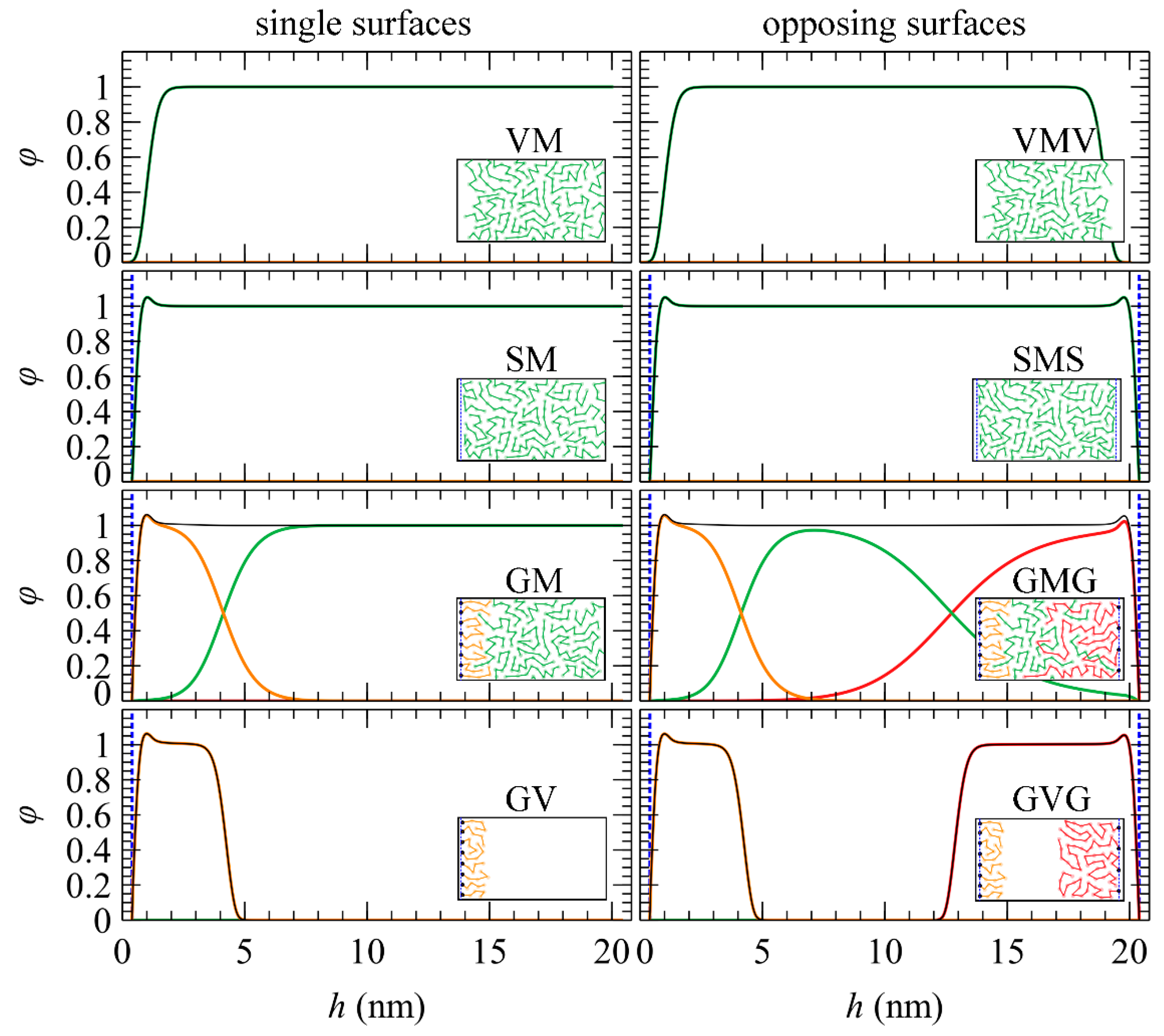
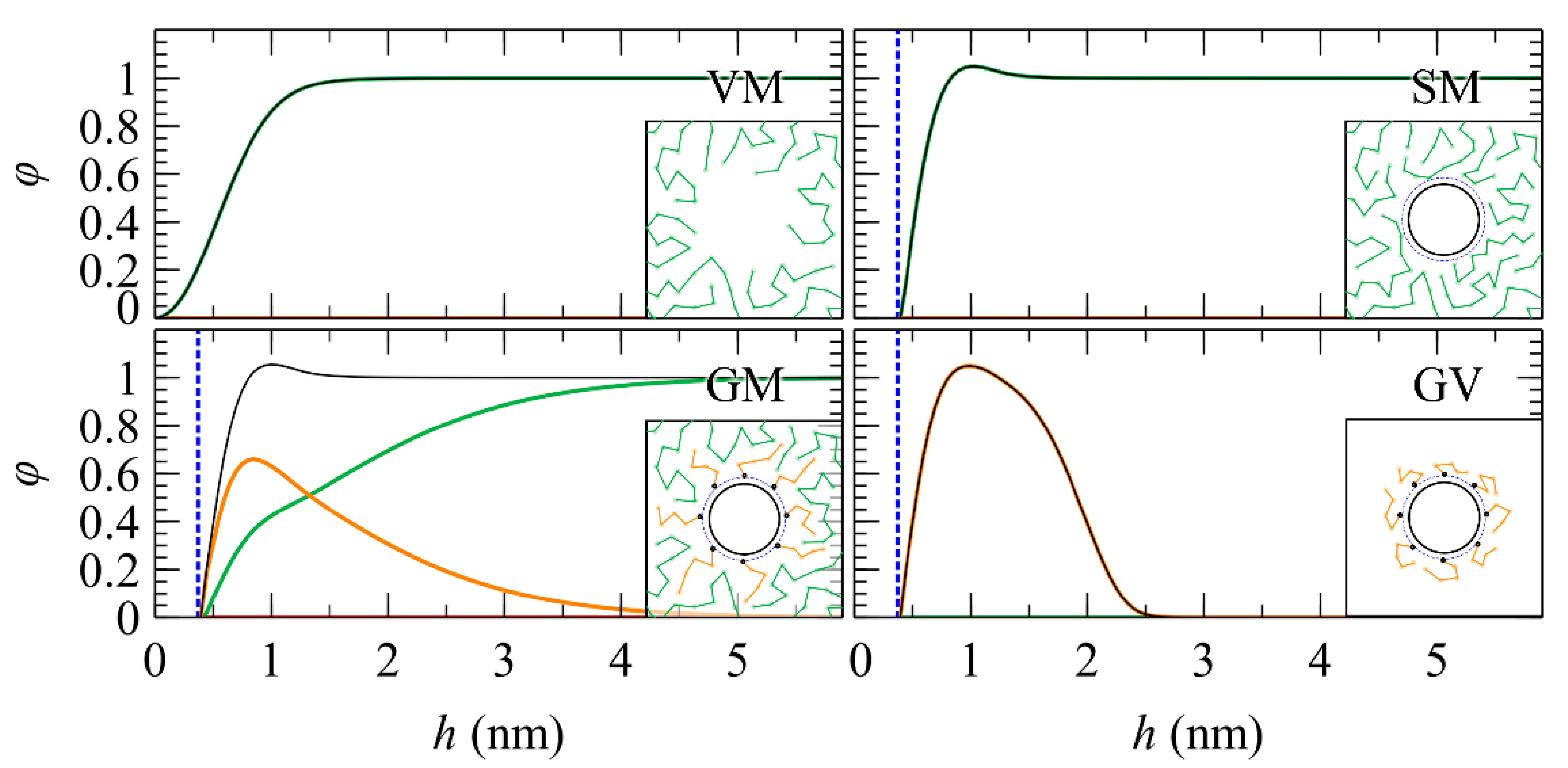
2.1. Geometries and Interfaces

At the moment, the code can support three kinds of chains (c) at the same time: matrix chains (c = m), and grafted chains at the low/high boundary (c = g ). The lengths of the matrix (Nm) and grafted ( N g ) chains, as well as the corresponding grafting density at each surface ( σ g ), can be tuned independently of each other. The type of the interface (i.e., gas vs. solid) is set by choosing the appropriate boundary conditions for each chain kind at the interfaces. Dirichlet boundary conditions, qc(r, N) = 0, are applicable for polymer–vacuum and polymer–solid interfaces, where r Ω . Neumann boundary conditions, r q c ( r , N ) = 0 , are applicable for boundaries corresponding to bulk phases (of melt or gas). In addition, the user can choose between planar and spherical geometries, corresponding to planar interfaces or films and nanoparticles or cavities, respectively. The flexibility of tuning these parameters individually enhances the accessible model space considerably.
To facilitate the discussion, the different kinds of boundaries and domains will be denoted as V: vacuum, S: solid surface, G: grafted (solid) surface, and M: melt or matrix; whereas combinations of these will be used to refer to each system. Figure 1 depicts illustrations and density profiles of representative planar geometries with single and opposing surfaces. Similarly, Figure 2 depicts some representative systems for spherical geometries (cavities and nanoparticles).
Setting vacuum interfaces at one or both sides of the domain allows for the modelling of vacuum–matrix interphases (Figure 2, VM) or free films (Figure 2, VMV), respectively [10,11,33,37]. In planar geometries, besides the density profiles and other relevant structural properties, one can estimate the interfacial free energy, that is, the surface tension, in this case. In spherical geometries (Figure 2, VM), the system corresponds to a cavity of radius R embedded in a melt, from which one can estimate the curvature-dependent structural properties of the polymer and the corresponding surface tension; hence, one can obtain a measure regarding the stability of the cavity.
On the other hand, introducing the polymer–solid interactions allows for the modelling of solid–polymer interphases, for example, see SM in Figure 1 and Figure 2. The wettability of these interphases can be tuned by adjusting the kind and the strength of the polymer–solid interactions; we elaborate on this subject in the next section. Enabling the solid interactions on both sides (Figure 1, SMS), allows for the estimation of the potential of mean force (or the disjoining pressure) and thus, obtaining a measure of the stability of such systems [28,34,38].
Introducing grafted chains on one surface (Figure 1 and Figure 2, GM) allows for the modeling of dilute grafted nanoparticles as a function of σ g , N g , Nm, and curvature, and extracts several key structural (density profiles, brush thickness) and thermodynamic quantities [27]. By grafting both surfaces (Figure 1, GMG), one can estimate the potential of mean force as a function of the surface–surface distance, the chain lengths and grafting densities of the grafted chains, and the chain lengths of matrix chains.
Removing the melt phase entirely, we can model grafted surfaces or NPs in dry solvent conditions (Figure 1 and Figure 2, GV). Having calculated the interfacial energies of GM and GV systems, one can estimate the solvation free energy. GVG systems, on the other hand, can provide information about the structure of the so-called “particle solids” (in cases where the particles are extremely coarse) [31,39].
The user is, of course, not limited to choosing these combinations. For example, one might want to examine SMV [37] or even GMV systems.

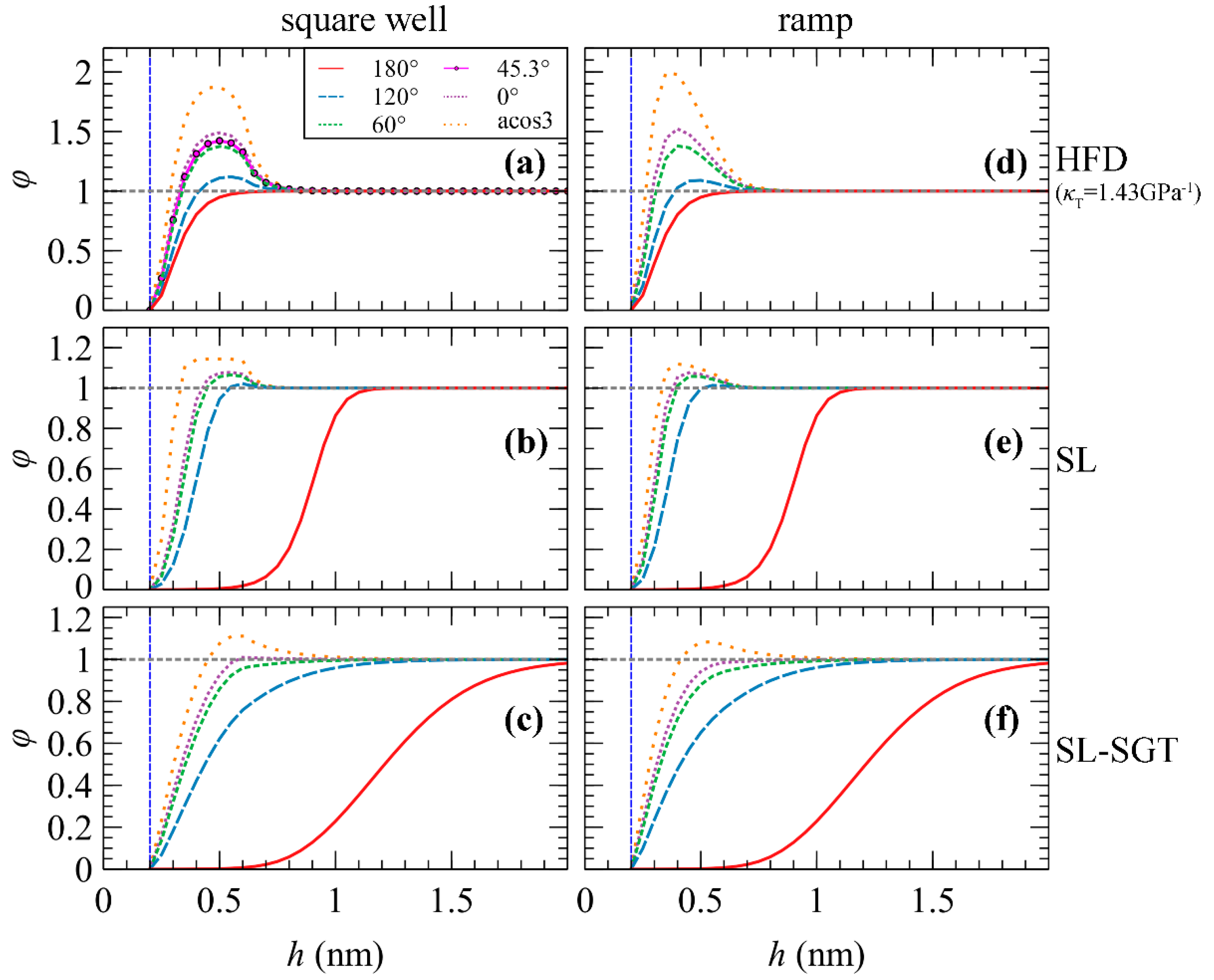
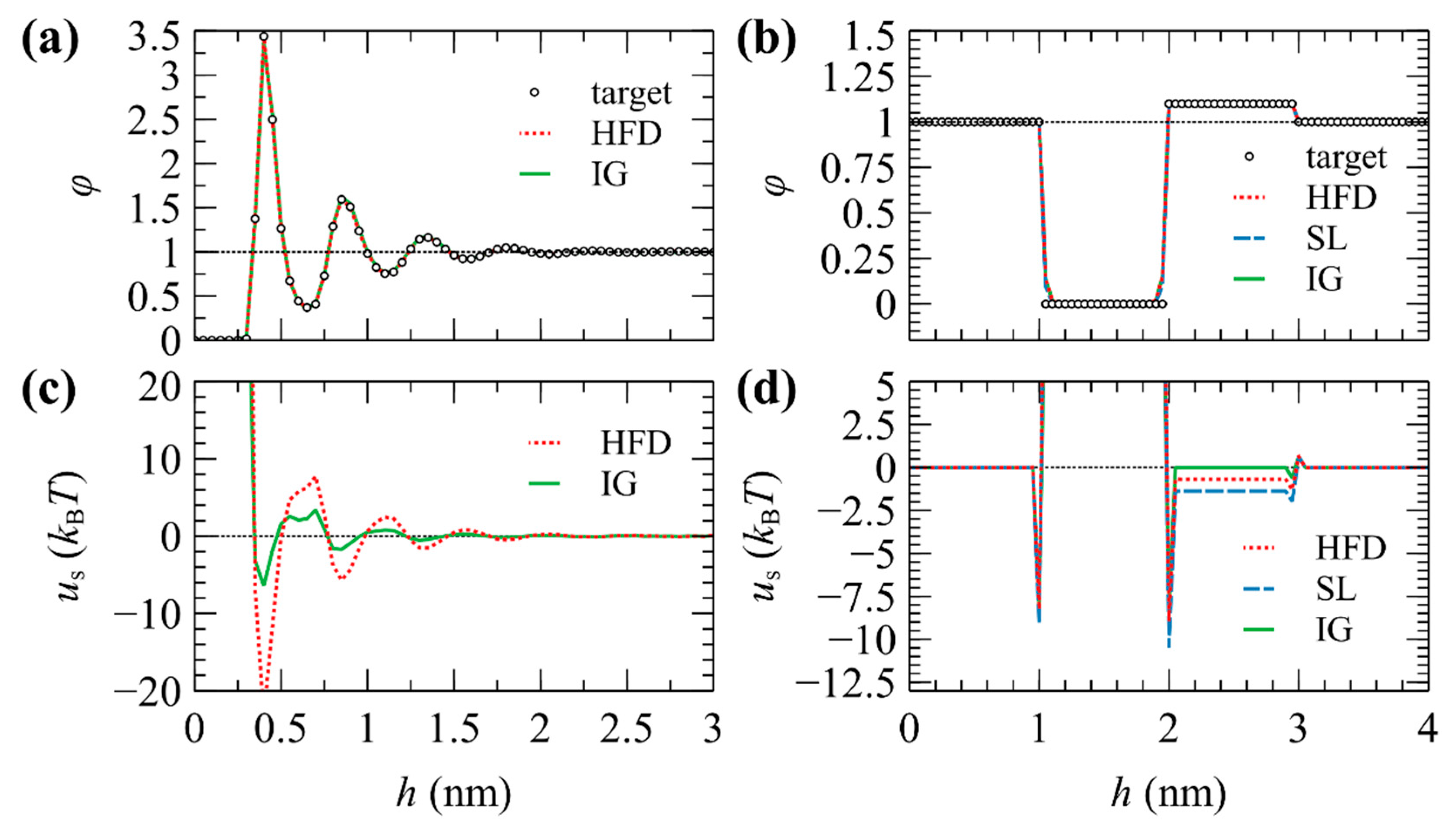
2.2. Polymer–Solid Interactions

In addition to the kind of boundary conditions, the code offers the possibility of selecting from a range of different wall potentials. In this way, the wetting degree of the interface can be altered according to the properties of the specific system that the user wishes to reproduce. The current section presents evaluations with the ramp, the square well, and tabulated potentials for demonstration purposes, but details concerning other functional forms, such as the Hamaker potential are also provided in the Supporting Information.
Figure 3 illustrates the density profiles of polyethylene (PE) melt near solid surfaces as a function of the contact angle using the HFD, SL, and SL-SGT EoS. The polymer–solid interactions have been described with the square well (vsquare_well, left) or the ramp (vramp, right) potential. The functional forms of the square well and ramp potentials are the following:
u square _ well = v square _ well     h < σ square _ well
u ramp = v ramp max ( σ ramp h σ ramp , 0 )
where vsquare_well/vramp and σsquare_well/σramp correspond to the depth and the width of the square well/ramp potential. The range of the potentials was set to 6.5 Å, and the position of the hard sphere wall at 2 Å (thus, the minimal distance of a segment from the hard sphere wall is equal to 4.5 Å) [10,32]. For each one of these cases, the depth of the potential was optimized with the Secant optimization method in order to match the target contact angles, θ = acos ( γ SM / γ VM ) , with γSM and γVM being the interfacial free energy of the SM and VM system, respectively. Note that, γVMσVM is the surface tension, and γSM ≡ –(σSV − σSM) [40] corresponds to minus the adhesion tension; thus, the contact angle can be estimated equivalently as θ = acos [ ( σ SV σ SM ) / σ VM ] .
In absence of solid surfaces (red lines in Figure 3, θ = 180°), the profiles exhibit a characteristic sigmoid shape, whereas the corresponding surface tension becomes γVM ~73.0, ~12.0, and ~29.5 mJ/m2, for HFD, SL, and SL-SGT, respectively [10,11]. In HFD, the isothermal compressibility has been set equal to κT = 1.43 GPa–1 [10,32], while the compressibility is roughly the same in the SL models (see Table S1 in Ref. [28]). The experimental surface tension of PE is 26.5–27.7 mJ/m2 [41], whereas the corresponding atomistic profile has a span of ~1 nm, [11]; thus, the SL-SGT model is more suitable for describing polymer–vacuum interfaces.
With increasing polymer–solid interactions (us) the profiles move closer to the solid surfaces and become more pronounced, especially when the HFD EoS is employed. Note that the profile with usquare_well for θ = 45.3° is identical to the corresponding profiles in Refs. [10,32].
Even though the compressibilities of these models are very similar, the density profiles from SL and SL-SGT EoS are more expanded because they take into consideration the probable formation of gas phases. In addition, they are less pronounced due to the existence of a logarithmic term that suppresses large fluctuations of the density above unity. In SL-SGT, the profiles are almost identical for the same contact angles regardless of the functional form of the potential (square well versus ramp).
Besides analytic functional forms, RuSseL supports tabulated potentials as well. Even though such potentials might be more cumbersome to work with, they are more flexible, in the sense that, in many cases, they allow for the reproduction of profiles of arbitrary shape.
For example, one can optimize the tabulated potentials to reproduce target density profiles, φtarget, via iterative Boltzmann inversion:
u s , i ( r ) = u s , i 1 ( r ) + a k B T ln ( φ i 1 ( r ) φ target ( r ) )
with a being a relaxation parameter. This process can be envisioned as reverse engineering the self-consistent field; instead of trying to predict the density profiles for a given field, the optimizer attempts to find the field that reproduces the target density profiles.
Figure 4a depicts a density profile at a polyethylene–graphite interface at 450 K obtained from molecular dynamics simulations [33] and the optimized density profiles from RuSseL using the HFD and the ideal gas (IG) free energy density; in the latter, the intermolecular interactions among chains are turned off, while the chain segments interact explicitly with the solid walls. The corresponding tabulated potentials are shown in Figure 4c. According to Figure 4a, it is possible to reproduce the MD profiles exactly, given that the underlying EoS does not impose any particular constraints. For example, it is impossible to reproduce these profiles with SL EoS since the logarithmic term does not allow the density to exceed the characteristic SL density. Similarly, Figure 4b depicts an exotic target density profile where φ = 0 for h [1, 2), φ = 1.1 for h [2, 3), and φ = 1 everywhere else. As with the previous case, the target profile has been reproduced with HFD, SL, and IG EoS in the presence of the corresponding tabulated potentials shown in Figure 4d.

3. Computational Details

3.1. Mathematical Formulation

The first step for the mathematical representation of the problem is to define the Hamiltonian of the system as a functional of the chemical potential field w, the segment density field, ρ, and the partition functions of matrix, Qm, and grafted chains, Qg relative to the field-free case. The methodology can also address systems comprising exclusively chains grafted on a solid surface, that is, not in contact with polymer melt. This is achieved by switching to a canonical ensemble formalism [28]. In this work, we limited the presentation of the mathematical formulation to cases where polymer melt is present. When matrix chains are present in the system, the grand canonical ensemble is most suitable for the thermodynamic description and the Hamiltonian, H, is given by Equation (4).
H [ ρ ( r ) , ρ ( r ) , w ( r ) ] = d r { i w ( r ) ρ ( r ) + f [ ρ ( r ) , ρ ( r ) ] + u s ( r ) ρ ( r ) } 1 β exp ( β μ m N m ) A m Z m , free V Q m [ i w ( r ) ] 1 β i g = 1 n g ln ( A g Z g , free Q g [ r g , i g ; i w ( r ) ] )
where μm is the chemical potential per segment of matrix chains, us describes the polymer segment–solid interactions, and f is an excess free energy density functional, which is used to describe the nonbonded cohesive interactions among the polymer segments. V is the volume occupied by polymer in the system; ng is the number of grafted chains, each grafted at position r g , i g ; Nm and Ng are the lengths of matrix and grafted chains, in segments; Zm,free and Zg,free are partition functions of field-free matrix and grafted chains, respectively; β = 1/kBT, where kB is the Boltzmann constant and T the temperature of the polymer melt; and A m and A g are normalizing factors.
In order to reduce the complexities arising from the functional integration of the spatially varying fields w and ρ, it is plausible to neglect the fluctuations of the fields by invoking a saddle-point approximation (also known as “mean-field approximation”), and to maintain only the configuration of the fields with the maximum statistical weight in the expression for the grand potential in terms of the Hamiltonian of Equation (4) [42]. In doing so, the interactions between the polymer segments are replaced with the interaction of each individual segment with the mean-field, which is generated by the rest of the segments, and the segment density field is connected to the real field w = i w (since w is purely imaginary) via Equation (5).
w ifc ( r ) = w ( r ) w bulk = f [ ρ , ρ ] ρ | ρ = ρ ( r ) f [ ρ , ρ ] ρ | ρ = ρ seg , bulk f [ ρ , ρ ] ρ + u s ( r )
Since the SCFT addresses systems of long polymer chains and high-density melts, it is quite common to represent the polymer chains with the Gaussian thread model. Daoulas et al. [32] have studied the accuracy of the Gaussian thread model in comparison to the worm-like chain model for the thermodynamic description of semi-flexible polymer melts at interfaces using SCFT. When chains are mathematically described as Gaussian threads, their conformations are governed by the Edwards diffusion Equation (6) [43,44].
N q c ( r , N ) = R g , c 2 N c r 2 q c ( r , N ) β w ifc ( r ) q c ( r , N )   ( c = m ,   g ,   g + )
where the solution, qc, is the restricted partition function for chains of kind c [10,11,27,32,42]; Rg,c is the radius of gyration of a polymer chain of kind c; N is the variable spanning the contour of the chain; Nc, as in Equation (4), is the length of a chain of kind c in monomer segments; and w ifc ( r ) , as in Equation (5), is the self-consistent field at a certain point r of the domain minus the corresponding value of the field in the bulk polymer region [27]. The code offers the possibility to solve Equation (6) for any thermoplastic polymer, providing the appropriate value for the parameter of the “diffusion coefficient” R g , c 2 / N c and the parameters for the EoS used to calculate the excess free energy density, for both matrix and grafted chains; the difference between the two cases being that they require different initial conditions. In the case of matrix chains, the initial conditions across the domain are given by Equation (7):
q m ( r , 0 ) = 1
Whereas, for the grafted chains, Equation (8) holds:
q g ( h g , 0 ) = S solid S h g σ g N g ρ seg , bulk δ ( h h g ) q m ( h g , N g )
where ρseg,bulk is the density of polymer segments in the bulk region, σg is the areal density of grafted chains and h g is the position of the grafting point of the grafted chain. The ratio of solid to grafting surface areas appearing in front of the right-hand side of eq 8 departs from unity only in nonplanar geometries. The value of the delta function is evaluated geometrically as the inverse of the interval length assigned to the grafting node of the 1D spatial mesh; for more details, see Section 2.1.2 of Ref. [27].

3.2. Discretization of the Edwards PDE

3.2.1. Semi-Implicit Finite Differences Discretization

In several works [10,18,32], the Crank–Nicholson contour discretization is implemented, which is a semi-implicit scheme (also known as “central differences”), in that the unknown solution, q h N , is expressed in our implementation by means of a central differences scheme, averaged between two successive contour points, N and NΝ, as shown in Equation (9).
2 q h 2 = 1 2 q h + 1 N + 1 2 q h N + 1 + q h 1 N + 1 Δ h 2 + 1 2 q h + 1 N 2 q h N + q h 1 N Δ h 2
while the first derivative of the solution, q, with respect to the contour variable N is given by Equation (10).
q h N = q h N + 1 q h N Δ N
Therefore, the matrix form of the partial differential Equation (6) to be solved becomes as follows:
D q h 1 N + 1 + ( 1 + 2 D + Δ N β w ifc , h 2 ) q h N + 1 D q h + 1 N + 1 = D q h 1 N + ( 1 2 D Δ N β w ifc , h 2 ) q h N + D q h + 1 N
with D = R G , c 2 Δ N 2 N c Δ h 2 being the diffusion coefficient.
In matrix-vector notation, Equation (11) can be written as presented in Equation (12).
( I D T + Δ N 2 W ) q N + 1 = ( I + D T Δ N 2 W ) q N
where I is the identity matrix and we have defined the matrices T and W, which are shown below:
T = [ 2 1 1 1 2 1 1 2 1 1 2 1 1 1 2 ]
W = [ w ( 0 ) w ( Δ h ) w ( 2 Δ h ) w ( L Δ h ) w ( L ) ]
Alternatively, Equation (12) can be written in terms of the stiffness matrix, K = I D T + Δ N 2 W , and the vector denoting the right-hand side, R = ( I + D T Δ N 2 W ) q N (i.e., the solution vector at the previous contour-step weighted with I + D T Δ N 2 W ), as follows:
K q N + 1 = R [ b 1 c 1 a 1 a 2 b 2 c 2 a 3 b 3 c 3 a n 1 b n 1 c n 1 c n a n b n ] [ q 1 N + 1 q 2 N + 1 q 3 N + 1 q n 1 N + 1 q n N + 1 ] = [ R 1 R 2 R 3 R n 1 R n ]
where a i = D , b i = 1 + 2 D + Δ N β w ifc , h 2 and c i = D . Note that Equation (15) has been written in the general form, without imposing any boundary conditions; all nodes are equivalent and as a result, the domain is periodic.

3.2.2. Implicit Finite Differences Discretization

A more stable, but computationally more demanding, way to solve the time-dependent partial differential equation is to express the unknown solution, q h N , in terms of the next contour step, NN, according to Equation (16), presented below.
2 q h 2 = q h + 1 N + 1 2 q h N + 1 + q h 1 N + 1 Δ h 2
In both cases, a linear system of equations needs to be solved to determine the solution at each contour step, but this implicit contour stepping method (also known as “backward differences”) allows for larger contour steps without reaching the numerical stability limits of the semi-implicit case. The first derivative of the chain contour is still given by Equation (10).
Adopting this discretization scheme, we end up with the following matrix-form of the partial differential equation to be solved:
2 D q h 1 N + 1 + ( 1 + 4 D + Δ N β w ifc , h ) q h N + 1 2 D q h + 1 N + 1 = q h N
where, again, the diffusion coefficient is given by the expression, D = R G , c 2 Δ N 2 N c Δ h 2 . In matrix-vector notation, Equation (17) is written as:
( I 2 D T + Δ N W ) q N + 1 = q N
where I is the identity matrix, and the matrices T and W are, again, those presented inEquation (14). In contrast to the semi-implicit scheme developed in the previous section, in the implicit one, the right-hand side is just the solution vector of the previous contour-step. As a result, eq 15 transforms as follows: a i = 2 D , b i = 1 + 4 D + Δ N β w ifc , h , c i = 2 D , and R = q N .

3.3. Boundary Conditions

In formulating the matrices presented above, we have not taken into consideration the boundary conditions that occur from the physics of the problem. Given the single dimensionality of the systems addressed by the version of RuSseL presented in this work, the system is mathematically represented by a line, which is bounded by one point on the left and another one on the right. In most cases where aperiodic systems are addressed, at least one of the bounding points needs to be assigned a Dirichlet boundary condition (also known as an “essential” or “absorbing” boundary condition). The physical interpretation of this type of condition is that the polymer melt is in contact with a solid or gas surface, and thus, the polymer segments are not allowed to reach that surface. On the other point of the domain, we can assign either a Dirichlet boundary condition as well, or a Neumann boundary condition and, therefore, specify a certain value for the derivative of the solution rather than the solution itself. If the right-hand side point denotes the position where the bulk region starts and the system is symmetric, then the solution derivative is set equal to zero. In order to demonstrate these considerations, we present the linear system of equations to be solved, in the case where Dirichlet or Neumann boundary conditions are imposed on both boundary points. For simplicity, we impose the boundary conditions at the nodes lying at the edges of the domain; it is possible, however, to apply them anywhere across the domain, as we demonstrate in Section 5.3. and 5.4.

3.3.1. Dirichlet–Dirichlet System

In a system with Dirichlet BC at i = 1 and i = n, eq 15 becomes the following:
[ 1 0 0 a 2 b 2 c 2 a 3 b 3 c 3 a n 1 b n 1 c n 1 0 0 1 ] [ q 1 q 2 q 3 q n 1 q n ] = [ R 1 DIR R 2 R 3 R n 1 R n DIR ]
In practice, applying the Dirichlet BC to the ith node entails the following substitutions: ai = 0, bi = 1, ci = 0, and R i = R i DIR (corresponding to a fixed qi value).

3.3.2. Neumann–Neumann System

If zero-derivative Neumann boundary conditions are imposed on the left (i = 1) and right (i = n) edges of the domain, then the matrix T needs to be modified, which, in turn, influences the final stiffness matrix and the right-hand side vector.
For the semi-implicit scheme, the matrix T is given by Equation (20):
T = [ 1 1 0 1 2 1 1 2 1 1 2 1 0 1 1 ]
Whereas, for the implicit scheme, it is given by Equation (21).
T = [ 2 2 0 1 2 1 1 2 1 1 2 1 0 2 2 ]

3.4. Solving the Linear System of Equations

In the case of non-periodic systems (a1 = cn = 0), where the stiffness matrix assumes a tridiagonal form, the linear system of equations is solved with the Thomas algorithm [45]. As in the conventional lower-upper (LU) decomposition algorithm, the solution of the tridiagonal system comprises three essential steps: decomposition, forward substitution, and backward substitution, which are presented below:
Decomposition:
a i a i b i 1 b i b i a i c i 1   ,   i = 2 , , n 1
Forward substitution:
R i R i a i R i 1 ,   i = 2 , , n
Backward substitution:
q n N + 1 R n b n q i N + 1 R i c i q i + 1 N + 1 b i ,   i = n 1 , , 1
On the other hand, when considering periodic systems, the linear system of equations is solved with a more general (but computationally more expensive) solver, which is based on the traditional Gauss elimination method with pivoting functionality [46].

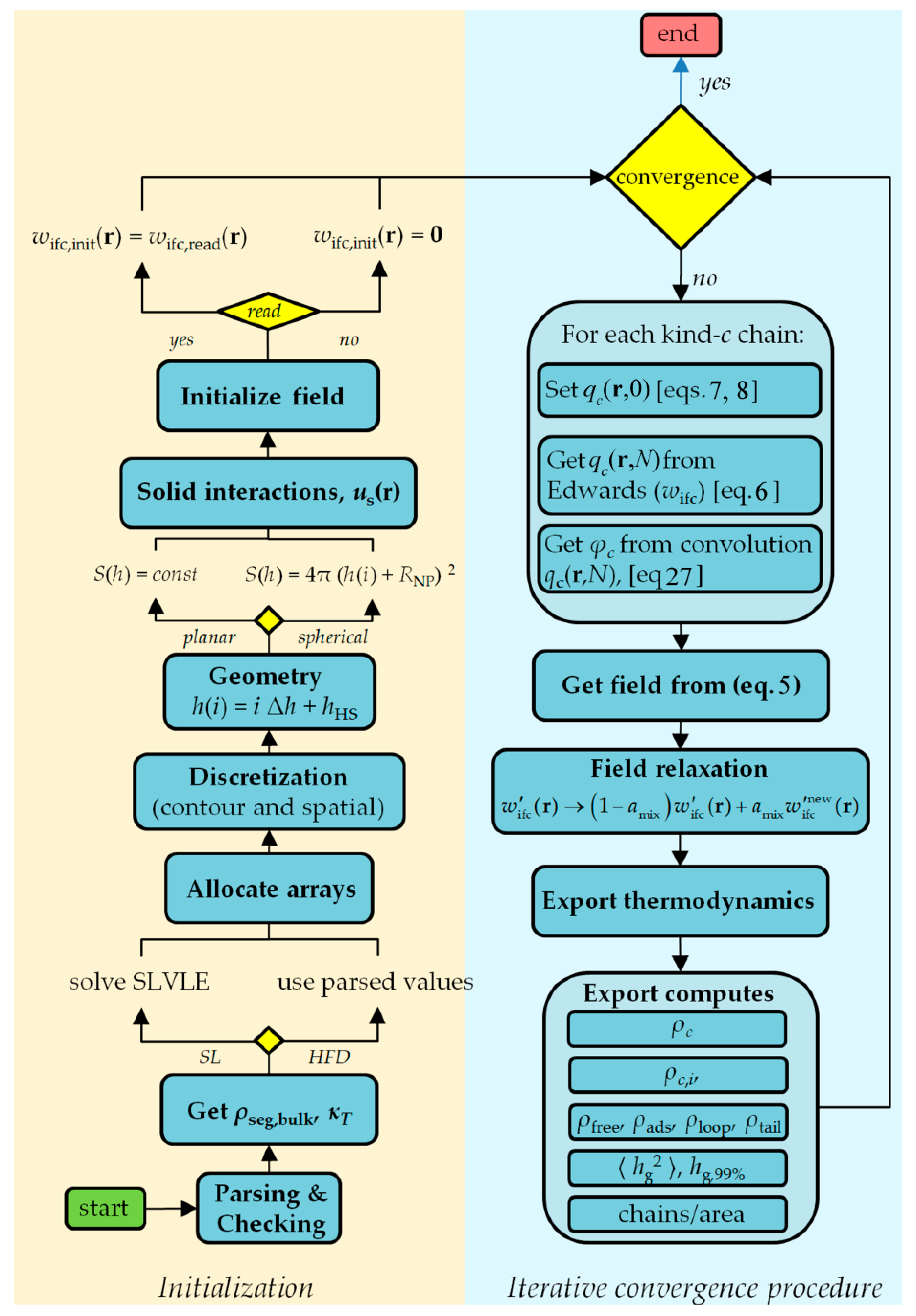
4. Code Structure and Description

The code was written in Fortran95 and it can be compiled and run both on Windows and Linux systems. The code is modular, extensible, and the subroutines have been abstracted in a way that makes them reusable. The models and calculation parameters are entirely controlled through an input file, which is parsed during runtime and contains information concerning the polymer physics, the discretization of space and chain contour, and the convergence parameters.

4.1. Input Files

During the initialization phase, the code attempts to read an input script by a dedicated subroutine, which parses the input file line-by-line and searches for special IDENTIFIERS that are related to specific user commands and operations. Whenever an IDENTIFIER is spotted, the program attempts to record the arguments(s) that precede it. In cases where an input line lacks any special IDENTIFIER or starts from “#” or “!”, it is skipped; thus, with very few exceptions, the order of the commands does not matter.
In addition, the parser has been equipped with an error-checking section that checks (i) whether the user has specified all the necessary inputs (e.g., domain size (L), temperature (T), geometry), (ii) the viability of individual user inputs (e.g., “are T or ρmass,bulk > 0?”, or “does a specific option exist?”), and (iii) whether the combinations of the inputs are viable (e.g., “is the grafting point located above the reflective wall?”). In cases where it finds a problem with the user inputs, the program issues a relevant error message and terminates.
The user has to initially specify the parameters of the domain, such as its size, geometry (planar, spherical), and boundary conditions (e.g., Dirichlet or Neumann), as well as other model-specific parameters, such as whether matrix or grafted chains are present in the system and the corresponding chain lengths, and thermodynamic conditions, such as the temperature and pressure. For spherical geometries the radius of the sphere, RNP, is also required.
The mass of the polymer chains and the coarse-graining degree are set by the molecular weight of the monomer constituting the polymer chains, mmonomer, whereas the radius of gyration of the chains is set indirectly based on the following relation [44]:
R g , c 2 N c = 1 6 C l C - C 2
with C being the characteristic ratio and lC-C being the chemical bond length between consecutive polymer segments provided by the user.
If calculations regarding solid–polymer interfaces are to be performed, then the user must select the sides of the walls (low, high, or both) and the functional form of the potentials that describe these interactions. So far, the code supports the following potential styles: Vacuum (no potential), Hamaker potential (sphere–sphere, sphere–plate, plate–plate) [27,35,36,47], Square well, Ramp, Tabulated, Hybrid, and Custom. The Tabulated potential allows the user to input a potential table that includes the polymer–solid interactions as a function of the distance of a segment from the solid surface. The hybrid style allows the user to enable several functional forms at the same time. Finally, the custom style allows the user to implement a custom functional form by specifying the list of coefficients in the input file. The functional form, however, must be specified in compile time. For more details, see Supplementary Information.
The cohesion of the polymer is specified by assigning an appropriate EoS coupled with its necessary parameters. So far, the code offers the possibility to run SCFT calculations using the Helfand (HFD) [48] and the Sanchez–Lacombe (SL) [49] equations of state. In addition, the free energy densities can be combined with a square gradient term to more accurately address polymer–gas interfaces [11,50]. Nevertheless, the code has been written in a generic way, so that any other appropriate model can be inserted and used [27]. In general, our code is able to run SCFT calculations for any thermoplastic polymer melt, given that an appropriate EoS coupled with its necessary parameters is provided.
The stability of the iterative convergence scheme can be enhanced by adjusting several parameters such as the following:
  • the contour length and spatial discretization (Δh, ΔΝc)
  • the kind of discretization (uniform, nonuniform)
  • the integration method (Simpson’s method, rectangle rule)
  • the field relaxation parameter amix, which depends on the isothermal compressibility, κT, of the bulk polymer and the length of the polymer chains [27]
  • the chain contour stepping method for the solution of the time-dependent PDE must be specified, that is, semi-implicit (also known as “Crank–Nicholson”) or implicit (see Section 3.2.1 and Section 3.2.2) [51].
The convergence criteria are based on the maximum number of iterations and the tolerance in the maximum error of the field, Δ w ifc tol .

4.2. Code Flow

The flow chart in Figure 5 illustrates the structure and overall flow of the RuSseL code. The code can be split into two main sections: (i) the initialization sections, and (ii) the iterative convergence procedure.
During the initialization phase, the code parses the input file and checks for user errors. When the HFD EoS is selected, ρmass,bulk and κT are assigned the input values at the given temperature and pressure, whereas, for the SL-EoS, these are estimated automatically based on the Sanchez–Lacombe vapor–liquid equilibrium (SLVLE) of the fluid and the input characteristic density, temperature, and pressure (see SI in Ref. [11]). After allocating and initializing the required arrays, the program implements the spatial and contour length discretization based on the user inputs. Subsequently, the code sets the wall–segment distance based on the coordinates of the hard-sphere wall (either via the input values or based on the automatic recalibration) and then computes the surface area of each layer S(h) and the system volume, V, based on the specified geometry. The program then sets the kind and the coefficients of the polymer–wall interactions of each solid surface, and then initializes the self-consistent field, either to zero or by reading it from an input binary file (useful for restarting a calculation).
Subsequently, the program enters the iterative convergence procedure until the convergence criteria are satisfied. At the start of each cycle and for each kind of chain (c = m, g, g+), the program computes the corresponding restricted partition function and reduced density as follows: (i) the partition function is initialized based on the boundary conditions and on Equation (7) or Equation (8) for matrix or grafted chains, respectively; (ii) the Edwards diffusion equation is evaluated for N up to Nc, subject to the field, w ifc , in planar or spherical geometries; (iii) the reduced density of the kind-c chains is calculated as follows:
φ c ( r ) = C ( q c , q m , N c , r )
with C being a convolution integral of the form:
C ( q a , q b , N c , r ) = 1 N c 0 N c d N   q a ( r , N )   q b ( r , N c N )
Next, the new field, w ifc new , is calculated from Equation (5) from the total reduced density, φ = φ m + φ g + φ g + , and is then relaxed based on the following mixing rule:
w ifc ( r ) ( 1 a mix ) w ifc ( r ) + a mix w ifc new ( r )
At a frequency that is specified by the user, the program exports the thermodynamic properties and computes. Finally, in case the convergence conditions are satisfied ( Δ w ifc tol < max ( { w ifc new ( r ) w ifc ( r ) , r R } )   or   N step > N step max ), the program exports the outputs and finalizes, or else the cycle of the iterative procedure restarts.

5. Export Computes

During the calculation, RuSseL offers the possibility to compute several properties regarding the thermodynamics of the system and the configurations of matrix and grafted chains. The export frequency of each compute can be adjusted by the user in order to save computational time and hard disk space. Unless otherwise stated, the present section will illustrate the exported quantities from a perfectly wetted PS-Silica system (same as Figure 1) in a GMV geometry with σ g = 0.4 nm–2, N g = 50, Nm = 100, and L = 10 nm.

5.1. Total and Partial Density Profiles

To begin with, useful quantities are the total (φtotal) and partial reduced density profiles of the grafted (φg) and matrix (φm), such as those shown in Figure 1, Figure 2 and Figure 6 for the GMV geometry examined here. With φ known, the segmental or the mass density profiles can be retrieved by multiplying φ with ρseg,bulk or ρmass,bulk of the corresponding polymer, respectively.

5.2. Brush Thickness

The dimensions of the grafted chains can be quantified in terms of the root mean square brush thickness:
h g 2 1 / 2 = [ R d h   h 2 ρ g ( h ) R d h ρ g ( h ) ] 1 / 2
and in terms of ⟨hg,99%⟩, which is defined here as the distance from the solid surface, which encloses 99% of the grafted chain segments:
R 99 % d h ρ g ( h ) = 0.99 N g n g

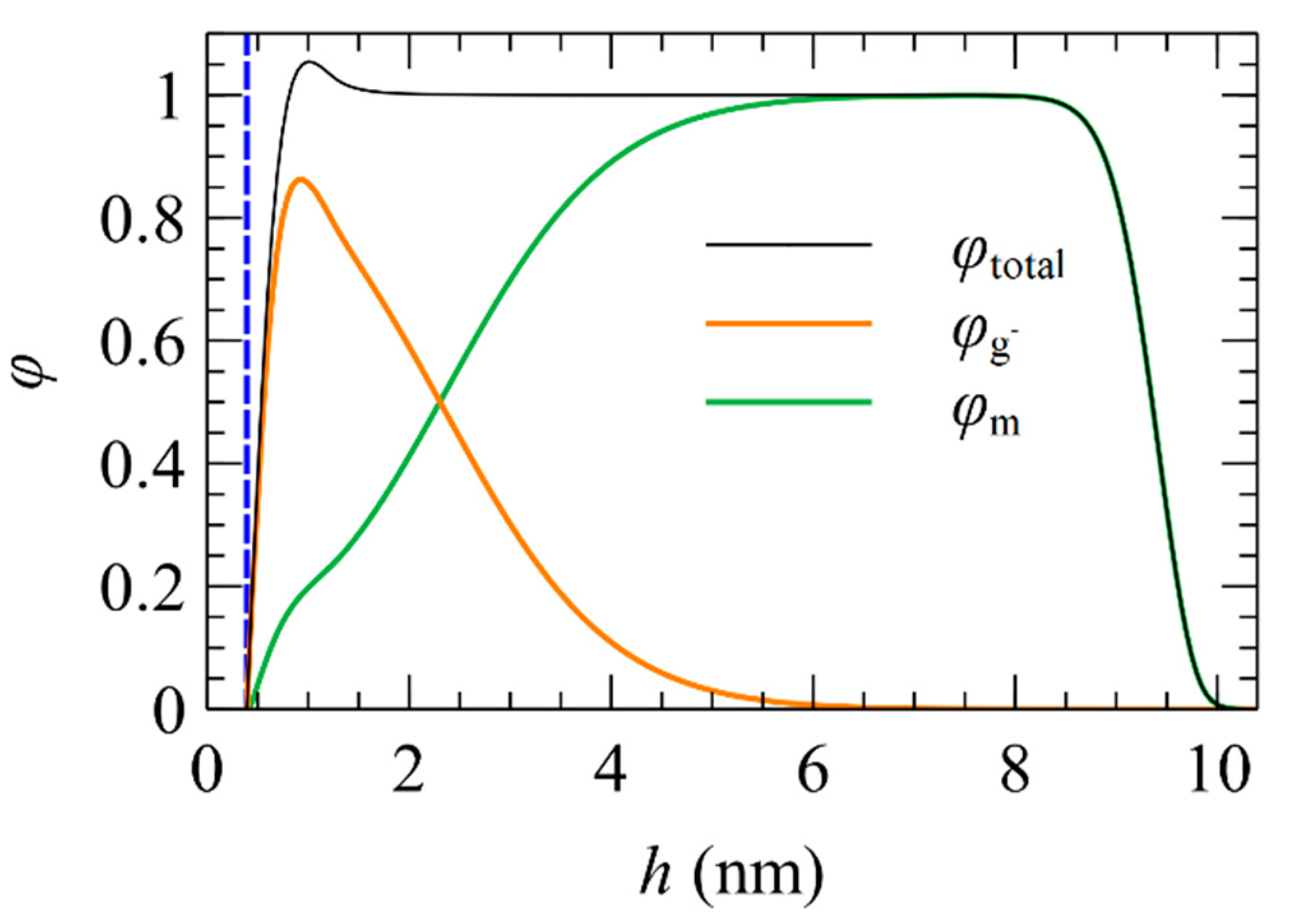
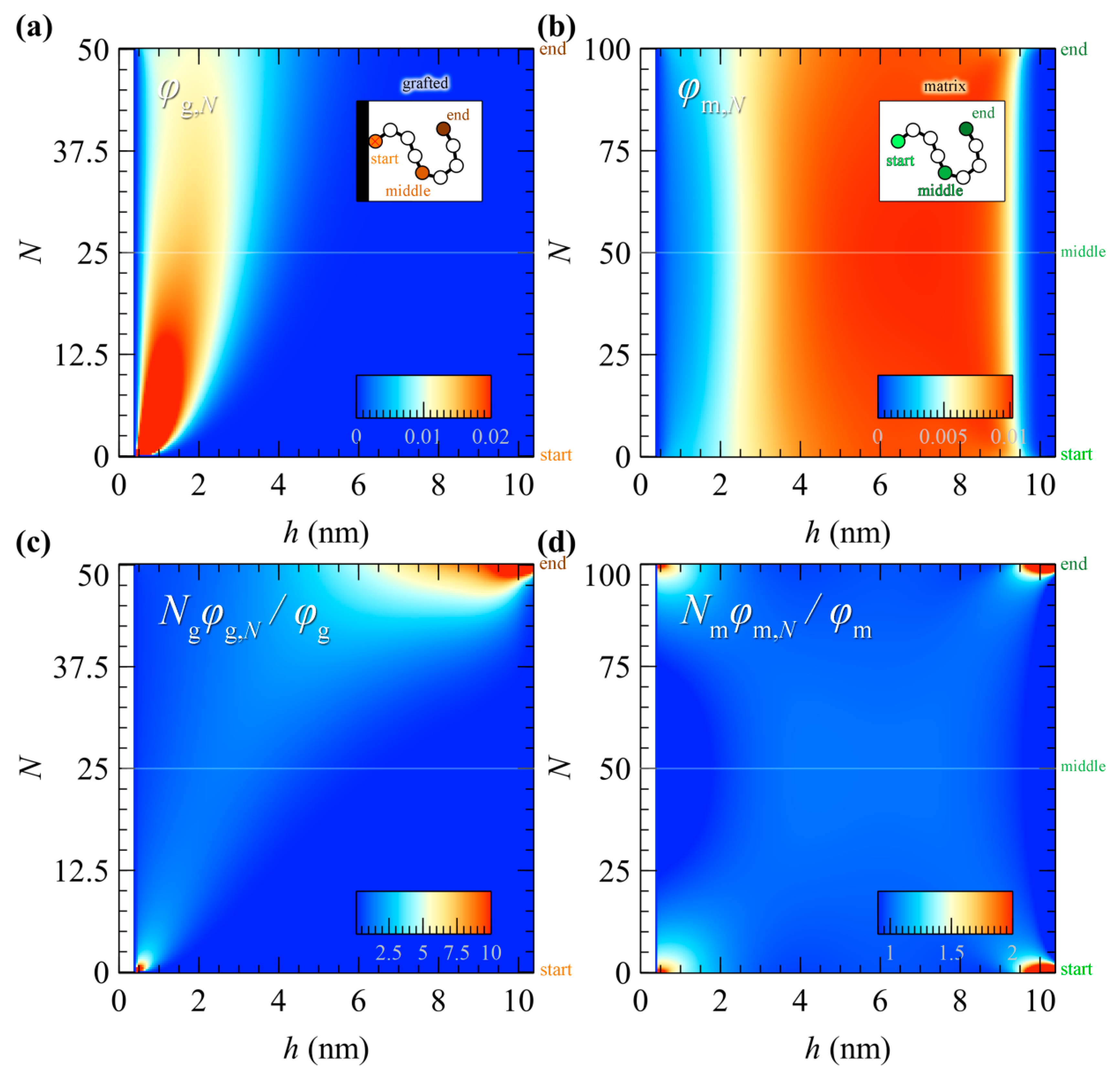
5.3. Profiles of Individual Chain Segments

Our code allows for the decomposition of the density profiles into contributions of individual chain segments, such as chain ends and middle segments [11,33,52]. The contribution of the Nth segment to the corresponding density profile of the kind-c chain can be retrieved by the following equation:
φ c , N ( r ) = 1 N c q c ( r , N )   q m ( r , N c N )
Setting N to 1 or Nc results in the density profile of the end segments, which can provide a very useful measure regarding the tendencies of the chain ends to segregate at the interfaces [11,27,33]. Setting N = Nc/2, on the other hand, results in the reduced density profiles of middle segments; comparisons among these two provide useful information regarding the overall shape of the chains [11].
Figure 7a depicts the segmental density profiles, φc,N, for the chain ends (N = 1, Nc) and middle segments (N = Nc/2) of grafted and matrix chains. The first segment of the grafted chains (N = 1) corresponds to the grafting point and features a sharp peak at h = hg. The middle segment and the last end segment of the grafted chains exhibit continuous density profiles, on the other hand, wherein the latter spreads further towards the matrix region. The density profiles of the matrix segments are suppressed in the vicinity of the grafted chains, since the latter reduce the available accessible space. Unlike grafted chains, the two end segments of the matrix chains are equivalent due to symmetry, hence their corresponding distributions are identical, φ m , 1 = φ m , N m . The ends of the matrix chains feature more pronounced profiles near the interfaces as compared to the middle segments.
These tendencies of the chain segments to segregate at the interfaces can be better quantified in terms of the normalized segment distribution, which is calculated via Equation (32).
φ ˜ c , N ( r ) = N c φ c , N ( r ) φ c ( r )
In practice, φ ˜ c , N ( r ) denotes the density of the Nth chain segments at a distance r, relative to the total segment density of the type-c chains; consequently, in a bulk phase, φ ˜ c , N = 1 .
According to Figure 7b, the segment density profiles of matrix chains become φ ˜ m , N = 1 , across the bulk region. Near the solid–polymer and the polymer–vacuum interfaces, the profiles of the end segments of the matrix chains are enhanced significantly by φ ˜ m , 1 ~ 6 and φ ˜ m , N m ~ 100, respectively, whereas the profiles of the middle segments are slightly less than bulk, φ ˜ m , N m / 2 < 1 . The corresponding profiles for the two ends of the grafted chains are highly asymmetric since φ ˜ g , 1 ~210 and φ ˜ g , N g ~ 0.6 at the grafting point, and φ ˜ g , 1 = 0 and φ ˜ g , N g ~ 180 at the edge of the free surface. The middle segments of the grafted chains exhibit suppressed profiles at the interfaces and over most of the matrix region. This effect is much more pronounced than for matrix chains; at the polymer–vacuum interface, φ ˜ g , N g / 2 1 .
Besides the end and middle segments, RuSseL allows for the exporting of the profile of any other segment specified by the user. The contour plots in Figure 8 depict φ c , N and φ ˜ c , N for all the segments of grafted and matrix chains.

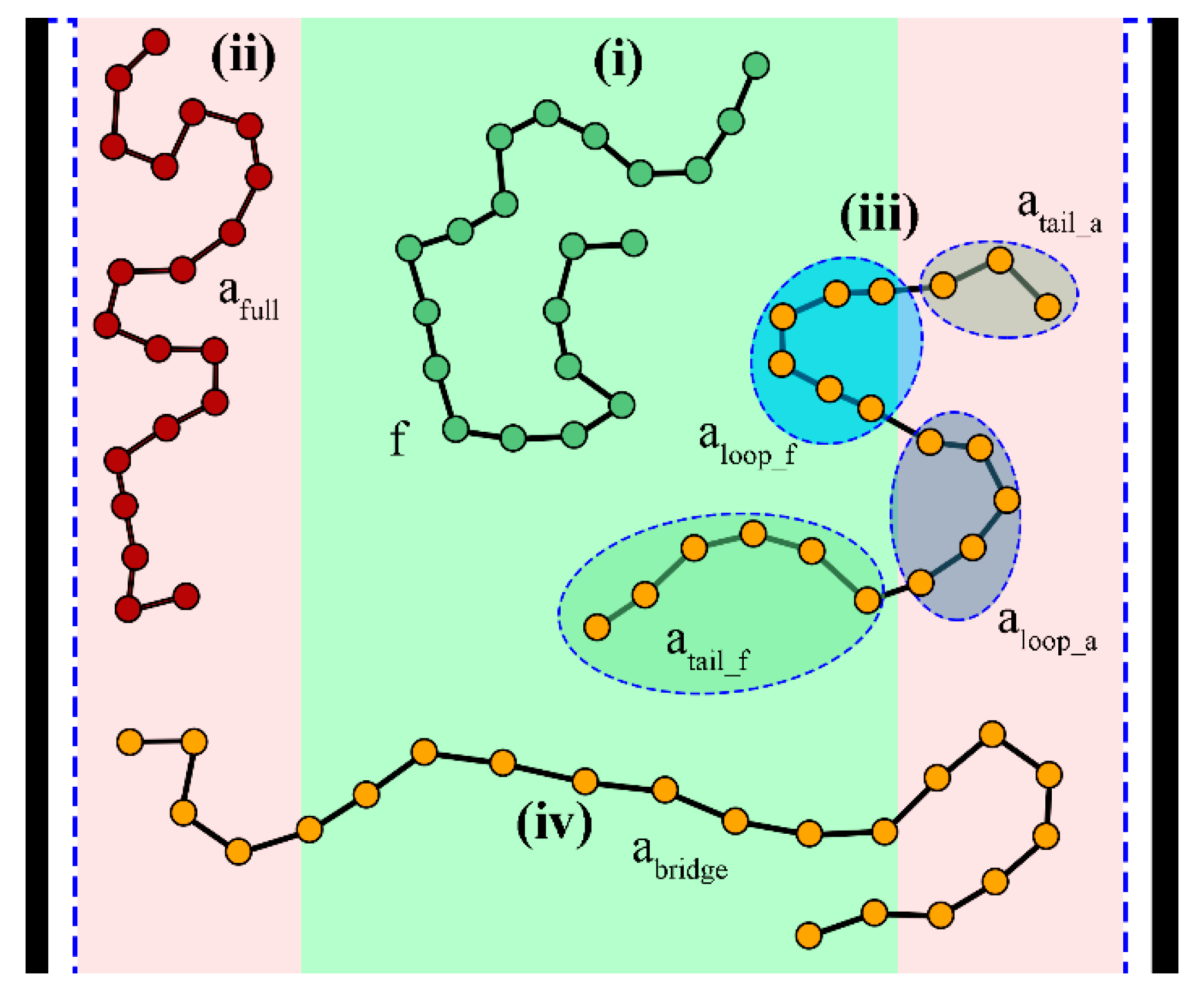
5.4. Distinction between Adsorbed and Free Segments

RuSseL has the option to decompose the density profiles into contributions of adsorbed and free segments based on segment surface distance criteria. Essentially, whenever a chain segment lies at a distance lower than h ads from the left (–) or right (+) surface, it can be classified as adsorbed to that surface. This is a purely geometric distinction based on a critical distance from the solid surface, which is defined by the user through the input file. There are several approaches to setting the critical distance, depending on the specific application:
  • Solid adsorption: hads can be tuned based on the peaks of the density profile (e.g., in Ref. [37], hads was set equal to 0.6 nm, the distance between the first two peaks of the polyethylene/graphite density profile), or based on the strength of polymer–solid interactions (e.g., in Ref. [28], hads was set equal to 1.28 nm, where the PS-Silica interactions, as described by the Hamaker potential, become very weak).
  • Segregation at polymer–vacuum interfaces: In Ref. [11], hads was set equal to a distance where the reduced density φ reaches 0.5.
  • Brush penetration: hads can also be set to the span of the grafted brush, hg,99%, in order to quantify the tendency of matrix chains to penetrate the brushes, or the tendencies of opposing brushes to penetrate each other.
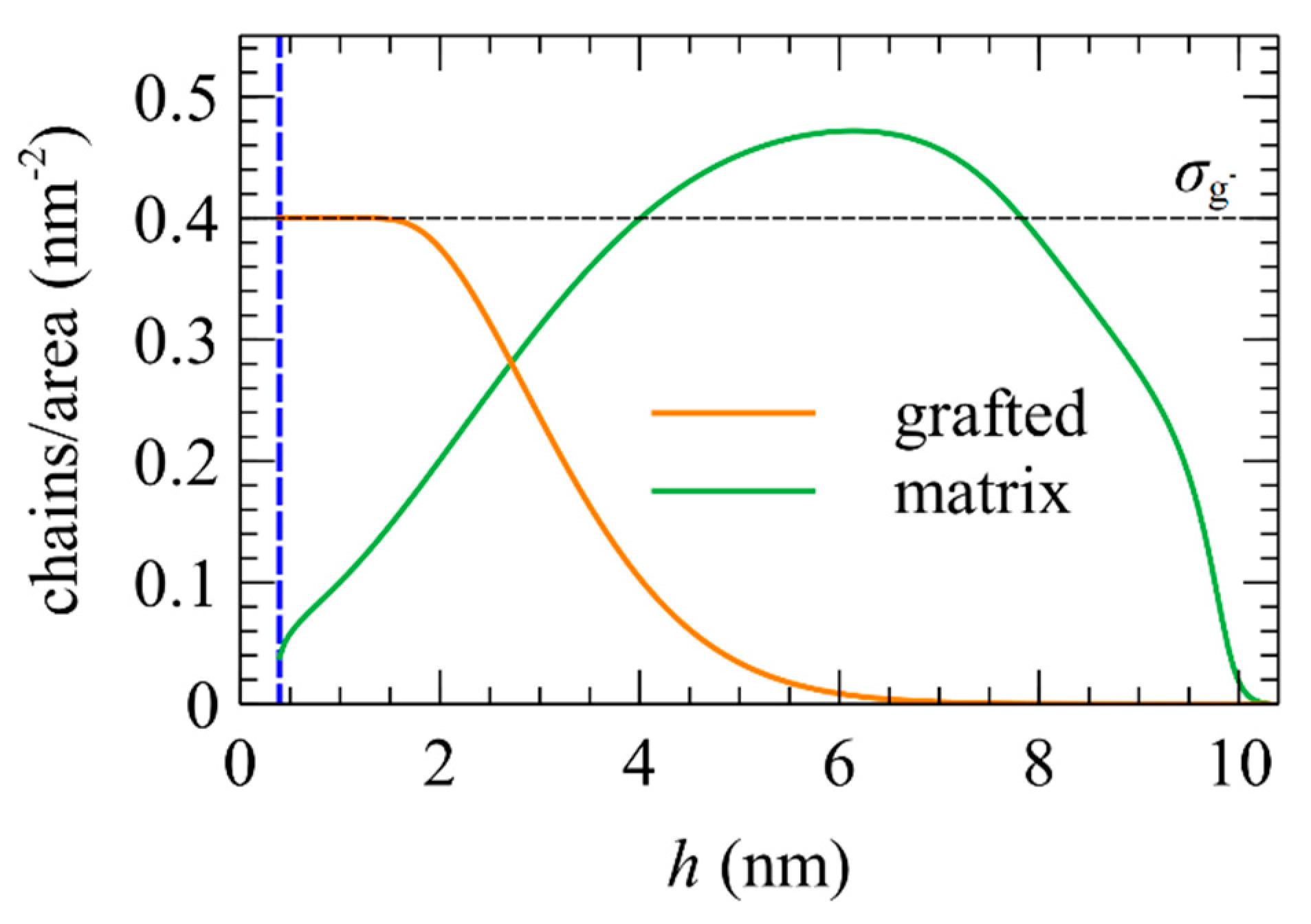
Based on the distribution of adsorbed and free segments of a chain, it is possible to classify the chain into several states and sub-states, which are denoted in Table 1.
A chain that is comprised entirely of free segments is classified as free (f); otherwise, in case it includes adsorbed segments, it is treated as adsorbed ( a ). The adsorbed chains can be classified into fully ( a full ) and partially ( a part ) adsorbed chains in cases where they are entirely or partially adsorbed to a surface. Furthermore, the free segments of partially adsorbed chains can be classified into free loops ( a loop _ f ) and tails ( a tail _ f ) and the adsorbed ones as adsorbed loops ( a loop _ a ) and tails ( a tail _ a ); the latter are also classified into trains [8,11,32,37]. Finally, a chain that is partially adsorbed in both surfaces can be classified as a bridge, a bridge . As can be imagined, the grafted chains cannot be classified to be free since, in most cases, the grafting points are located below hads; however, this procedure can unveil meaningful sub-states, such as fully and partially adsorbed grafted chains, as well as bridges.
Figure 9 includes some representative examples, whereas Figure 10 depicts the profiles of the aforementioned states from a perfectly wetted SMS system (see Table 1 in Ref. [27]) with h ads = h ads + = 6 nm, and plate–plate distance, hss~ 16.8 nm (L = 16 nm). In this calculation, h ads and h ads + have been chosen to be rather large, for illustrative purposes.
The first step of the classification procedure is to calculate the partition functions of the free ( q c f ), the fully adsorbed ( q c a full , q c a full + ), and the non-adsorbed ( q c ! a , q c ! a + ) chains with respect to the left (–) and the right (+) surface; for example, see Figure 10a. Note that a chain that is not adsorbed to a specific surface is not necessarily free since it might be adsorbed to the opposing surface.
To calculate each one of them, the Edwards diffusion equation is evaluated with the additional constraint that the Dirichlet boundary condition, qc(h, N) = 0, is set to all the nodes with distance, h, within the ranges specified at the rightmost column of Table 1. In other words, the Edwards diffusion equation is evaluated in such a way that the chains are unable to access these ranges of the domain. Subsequently, the density profiles corresponding to these states and sub-states are calculated with the convolution integrals and the relations specified in Table 1. C symbolizes convolution of the restricted partition functions indicated; compare Equation (27).
Note that, a loop states corresponding to free or adsorbed segments are denoted as a loop _ f and a loop _ a , respectively; hence, a loop = a loop _ f + a loop _ a . Moreover, note that the states have been defined in such a way that the following relations are satisfied:
φ c a = φ c a full + φ c a part
φ c a part = φ c a loop _ f + φ c a loop _ a + φ c a tail _ f + φ c a tail _ a
φ c = φ c a - + φ c a + + φ c f φ c a bridge
Note that the bridges are a measure of the overlap between profiles of the adsorbed chains at the opposing surfaces; thus, in situations that the separation distance of these surfaces is large enough, φbridge → 0.

5.5. Chains/Area

For both matrix and grafted chains, the number of chains per unit area can be determined, which is calculated through Equations (36) and (37). For the definition of this structural property, the reader is referred to previous works of authors [11,27,32,53].
p int , c ( h 0 ) = 1 R q c , h 0 shape ( h , N c ) d h R q c ( h , N c ) d h
n ch , c ( h 0 ) = p int , c ( h 0 ) 1 S h 0 1 N c R ρ c ( h ) d h
q c , h 0 shape is the restricted partition function of all the chains that are unable to cross the surface at h0, and it is calculated by evaluating the Edwards diffusion equation with the constraint that the Dirichlet boundary condition, qc(h, N) = 0, is applied at the node at h0. Subsequently, p int , c ( h 0 ) is the probability that a chain will intersect this surface, and nch,c(h0) corresponds to the number of type-c chains per unit area that pass through the surface at h0. Consequently, near the grafting points, the chains/area equal the grafting density, as illustrated by the dashed line in Figure 11.

5.6. Free Energy Density Components

The total free energy (grand potential) of the system is split into the following contributions:
Δ Ω = Ω Ω bulk A g , bulk = Δ Ω coh + Δ Ω field + Δ Ω m + Δ A g + U s + U ss
Note that the total free energy has been defined with respect to a bulk melt of matrix chains with the same length (Nm) and chemical constitution, and at the same temperature and pressure, and with respect to n g end-pinned unperturbed chains of length N g exposed to bulk melt. In cases where the matrix chains are absent, Ωbulk is zero. The cohesive interactions among the polymer segments (ΔΩcoh) are described by Equation (39), with f [ ρ ( r ) , ρ ( r ) ] being a free energy density term from an equation of state specified by the user. The interaction between the (total) segment density field, ρ(r), and the self-consistent field, w ifc ( r ) , is given by Equation (40). The total solid–polymer interactions (Us)—when present—are given by Equation (41); whereas, their functional form, us(r), is specified by the user. The free energies associated with the conformational entropy of matrix and grafted chains (if they exist) are given by Equations (42) and (43), respectively.
Δ Ω coh = R d r { f [ ρ ( r ) , ρ ( r ) ] f [ ρ seg , bulk , 0 ] }
Δ Ω field = R d r { ρ ( r ) w ( r ) ρ seg , bulk w bulk ( r ) }
U s = R d r { ρ ( r ) u s ( r ) }
Δ Ω m = ρ seg , bulk V β N m ( Q m [ w w bulk ] 1 )
Δ A g = 1 β i g = 1 n g ln Q g [ r g , i g ; w w bulk ] 1 β i g = 1 n g ln r ref , q = 0 r g , i g , q = 0
where β = 1/kBT. In systems with opposing solid surfaces, we introduce an additional enthalpic term that describes the solid–solid interactions. The functional form of this term depends on the potential of the solid.
With known adhesion tension and surface tension (from the corresponding VM system), one can compute the four macroscopic wetting functions of the interface as well as the corresponding contact angle at the solid–liquid–vapor interface [28,33].

6. Conclusions

An in-house code has been developed to perform calculations on one-dimensional domains based on Self-Consistent Field Theory and considering compressible polymer melts of Gaussian-thread chains. The code solves the Edwards diffusion equation using a Finite Differences scheme and it addresses heterogeneous polymer systems comprising homopolymer polymer melts in contact with gas or solid surfaces. In the latter case, the code offers the possibility to work with different potentials for the description of solid–polymer interactions, namely Hamaker, square-well, and user-specified potentials (either tabulated or analytic). There is also the option to choose from among the Helfand and the Sanchez–Lacombe equation of state, with or without square-gradient correction, for the description of the nonbonded interactions between the polymer segments. Building upon the content of our previous publications [11,27,28], we present the way that the code computes several thermodynamic and structural properties of the system.
The code has already been used by the authors in a number of publications regarding various systems, and this article, along with the accompanying manual, was written to serve as a technical reference for anyone who desires to reproduce the corresponding results. In this article, we have demonstrated a part of the capabilities of the code and validated our findings with results reported in the literature. There is plenty of room for future extensions of the code, for example, block copolymer systems, polydisperse polymer melts, additional models for nonbonded interactions (e.g., SAFT [54]), additional models for solid–polymer interactions, and investigation of more efficient solvers for the solution of the Edwards partial differential equations. The authors have also developed the three-dimensional analogue of RuSseL, implementing the Finite Element Method [25], which is also going to be published in the near future. The development of both versions of the code is an ongoing process and the authors are always trying to stay tuned and incorporate more computational tools and capabilities into their software, aiming to contribute to the area of polymer nanocomposites and shed light on several topics that still remain elusive to the community.

Supplementary Materials

The source code of RuSseL and its manual are available online at https://www.mdpi.com/article/10.3390/computation9050057/s1.

Author Contributions

Conceptualization, C.J.R., A.P.S. and D.N.T.; methodology, C.J.R., A.P.S., A.T.L. and D.N.T.; software, C.J.R., A.P.S. and A.T.L.; validation, C.J.R. and A.P.S.; formal analysis, C.J.R. and A.P.S.; investigation, C.J.R. and A.P.S.; resources, D.N.T.; data curation, C.J.R. and A.P.S.; writing—original draft preparation, C.J.R. and A.P.S.; writing—review and editing, D.N.T., C.J.R. and A.P.S.; visualization, A.P.S.; supervision, D.N.T.; project administration, D.N.T.; funding acquisition, D.N.T. All authors have read and agreed to the published version of the manuscript.

Funding

Financial support by the Hellenic Foundation for Research and Innovation (H.F.R.I), project number 1263, under the “First Call for H.F.R.I Research Projects to support Faculty members and Researchers and the procurement of high-cost equipment grant” is gratefully acknowledged. A.P.S. thanks SOLVAY, Paris, France, for financial support through the project “Multiscale Modeling for the Design of Antifouling Copolymers”. C.J.R. gratefully acknowledges financial support from the “Special Account for Research Funding” of the National Technical University of Athens and also through the project MuSiComPS, Grant Agreement 10062/19, sponsored by the LIMMAT Foundation, Switzerland. Part of this work was supported by computational time granted from the Greek Research and Technology Network (GRNET) in the National HPC facility—ARIS—under project ID pa201203 (MuSiPolI).

Data Availability Statement

Not applicable.

Conflicts of Interest

The authors declare no conflict of interest. The funders had no role in the design of the study; in the collection, analyses, or interpretation of data; in the writing of the manuscript, or in the decision to publish the results.

References

  1. Yan, L.-T.; Xie, X.-M. Computational modeling and simulation of nanoparticle self-assembly in polymeric systems: Structures, properties and external field effects. Prog. Polym. Sci. 2013, 38, 369–405. [Google Scholar] [CrossRef]
  2. Zeng, Q.H.; Yu, A.B.; Lu, G.Q. Multiscale modeling and simulation of polymer nanocomposites. Prog. Polym. Sci. 2008, 33, 191–269. [Google Scholar] [CrossRef]
  3. Chen, S.; Doolen, G.D. Lattice Boltzmann Method for Fluid Flows. Annu. Rev. Fluid Mech. 1998, 30, 329–364. [Google Scholar] [CrossRef] [Green Version]
  4. Español, P.; Warren, P.B. Perspective: Dissipative particle dynamics. J. Chem. Phys. 2017, 146, 150901. [Google Scholar] [CrossRef]
  5. Bore, S.L.; Kolli, H.B.; De Nicola, A.; Byshkin, M.; Kawakatsu, T.; Milano, G.; Cascella, M. Hybrid particle-field molecular dynamics under constant pressure. J. Chem. Phys. 2020, 152. [Google Scholar] [CrossRef] [PubMed]
  6. Caputo, S.; Hristov, V.; De Nicola, A.; Herbst, H.; Pizzirusso, A.; Donati, G.; Munaò, G.; Albunia, A.R.; Milano, G. Efficient Hybrid Particle-Field Coarse-Grained Model of Polymer Filler Interactions: Multiscale Hierarchical Structure of Carbon Black Particles in Contact with Polyethylene. J. Chem. Theory Comput. 2021, 17, 1755–1770. [Google Scholar] [CrossRef]
  7. Sgouros, A.P.; Vogiatzis, G.G.; Megariotis, G.; Tzoumanekas, C.; Theodorou, D.N. Multiscale Simulations of Graphite-Capped Polyethylene Melts: Brownian Dynamics/Kinetic Monte Carlo Compared to Atomistic Calculations and Experiment. Macromolecules 2019, 52, 7503–7523. [Google Scholar] [CrossRef]
  8. Sgouros, A.P.; Lakkas, A.T.; Megariotis, G.; Theodorou, D.N. Mesoscopic Simulations of Free Surfaces of Molten Polyethylene: Brownian Dynamics/kinetic Monte Carlo Coupled with Square Gradient Theory and Compared to Atomistic Calculations and Experiment. Macromolecules 2018, 51, 9798–9815. [Google Scholar] [CrossRef]
  9. Lo Verso, F.; Egorov, S.A.; Milchev, A.; Binder, K. Spherical polymer brushes under good solvent conditions: Molecular dynamics results compared to density functional theory. J. Chem. Phys. 2010, 133, 184901. [Google Scholar] [CrossRef] [PubMed] [Green Version]
  10. Theodorou, D.N.; Vogiatzis, G.G.; Kritikos, G. Self-consistent-field study of adsorption and desorption kinetics of polyethylene melts on graphite and comparison with atomistic simulations. Macromolecules 2014, 47, 6964–6981. [Google Scholar] [CrossRef] [Green Version]
  11. Lakkas, A.T.; Sgouros, A.P.; Theodorou, D.N. Self-Consistent Field Theory Coupled with Square Gradient Theory of Free Surfaces of Molten Polymers and Compared to Atomistic Simulations and Experiment. Macromolecules 2019, 52, 5337–5356. [Google Scholar] [CrossRef]
  12. Müller, M. Phase diagram of a mixed polymer brush. Phys. Rev. E Stat. Phys. Plasmas Fluids Relat. Interdiscip. Top. 2002, 65, 1–4. [Google Scholar] [CrossRef]
  13. Trombly, D.M.; Ganesan, V. Curvature effects upon interactions of polymer-grafted nanoparticles in chemically identical polymer matrices. J. Chem. Phys. 2010, 133, 154904. [Google Scholar] [CrossRef] [PubMed]
  14. Müller, M.; Schmid, F. Incorporating fluctuations and dynamics in self-consistent field theories for polymer blends. Adv. Polym. Sci. 2005, 185, 1–58. [Google Scholar]
  15. Ouaknin, G.; Laachi, N.; Delaney, K.; Fredrickson, G.H.; Gibou, F. Self-consistent field theory simulations of polymers on arbitrary domains. J. Comput. Phys. 2016, 327, 168–185. [Google Scholar] [CrossRef] [Green Version]
  16. Arora, A.; Qin, J.; Morse, D.C.; Delaney, K.T.; Fredrickson, G.H.; Bates, F.S.; Dorfman, K.D. Broadly Accessible Self-Consistent Field Theory for Block Polymer Materials Discovery. Macromolecules 2016, 49, 4675–4690. [Google Scholar] [CrossRef]
  17. Rasmussen, K.; Kalosakas, G. Improved numerical algorithm for exploring block copolymer mesophases. J. Polym. Sci. Part B Polym. Phys. 2002, 40, 1777–1783. [Google Scholar] [CrossRef]
  18. Drolet, F.; Fredrickson, G.H. Combinatorial screening of complex block copolymer assembly with self-consistent field theory. Phys. Rev. Lett. 1999, 83, 4317–4320. [Google Scholar] [CrossRef]
  19. Drolet, F.; Fredrickson, G.H. Optimizing chain bridging in complex block copolymers. Macromolecules 2001, 34, 5317–5324. [Google Scholar] [CrossRef]
  20. Kim, J.U.; Matsen, M.W. Finite-stretching corrections to the Milner-Witten-Cates theory for polymer brushes. Eur. Phys. J. E 2007, 23, 135–144. [Google Scholar] [CrossRef]
  21. Vigil, D.L.; García-Cervera, C.J.; Delaney, K.T.; Fredrickson, G.H. Linear Scaling Self-Consistent Field Theory with Spectral Contour Accuracy. ACS Macro Lett. 2019, 8, 1402–1406. [Google Scholar] [CrossRef]
  22. Ackerman, D.M.; Delaney, K.; Fredrickson, G.H.; Ganapathysubramanian, B. A finite element approach to self-consistent field theory calculations of multiblock polymers. J. Comput. Phys. 2017, 331, 280–296. [Google Scholar] [CrossRef] [Green Version]
  23. Huttom, D.V. Fundamentals of Finite Element Analysis; McGraw Hill: New York, NY, USA, 2004; ISBN 0-07-112231-1. [Google Scholar]
  24. Smith, I.M.; Griffiths, D.V.; Margetts, L. Programming the Finite Element Method, 5th ed.; Wiley: West Sussex, UK, 2014; ISBN 9781119973348. [Google Scholar]
  25. Revelas, C.J.; Sgouros, A.P.; Lakkas, A.T.; Theodorou, D.N. A Three-Dimensional Finite Element Methodology for Addressing Heterogeneous Polymer Systems with Simulations Based on Self-Consistent Field Theory. In Proceedings of the International Conference of Computational Methods In Science and Engineering 2020 (ICCMSE 2020), Heraklion, Crete, Greece, 27 April–3 May 2020; p. 130002. [Google Scholar]
  26. Daoulas, K.C.; Müller, M. Exploring thermodynamic stability of the stalk fusion-intermediate with three-dimensional self-consistent field theory calculations. Soft Matter 2013, 9, 4097–4102. [Google Scholar] [CrossRef]
  27. Lakkas, A.T.; Sgouros, A.P.; Revelas, C.J.; Theodorou, D.N. Structure and Thermodynamics of Grafted Silica/Polystyrene Nanocomposites Investigated Through Self-Consistent Field Theory. Soft Matter 2021, 17, 4077–4097. [Google Scholar] [CrossRef]
  28. Sgouros, A.P.; Revelas, C.J.; Lakkas, A.T.; Theodorou, D.N. Potential of Mean Force between Bare or Grafted Silica/Polystyrene Surfaces from Self-Consistent Field Theory. Polymers (Basel) 2021, 13, 1197. [Google Scholar] [CrossRef]
  29. Cheong, G.K.; Chawla, A.; Morse, D.C.; Dorfman, K.D. Open-source code for self-consistent field theory calculations of block polymer phase behavior on graphics processing units. Eur. Phys. J. E 2020, 43, 15. [Google Scholar] [CrossRef] [Green Version]
  30. Price-Whelan, A.M. SCF 1991. Available online: https://github.com/adrn/scf_fortran (accessed on 10 May 2021).
  31. Bilchak, C.R.; Buenning, E.; Asai, M.; Zhang, K.; Durning, C.J.; Kumar, S.K.; Huang, Y.; Benicewicz, B.C.; Gidley, D.W.; Cheng, S.; et al. Polymer-Grafted Nanoparticle Membranes with Controllable Free Volume. Macromolecules 2017, 50, 7111–7120. [Google Scholar] [CrossRef]
  32. Daoulas, K.C.; Theodorou, D.N.; Harmandaris, V.A.; Karayiannis, N.C.; Mavrantzas, V.G. Self-consistent-field study of compressible semiflexible melts adsorbed on a solid substrate and comparison with atomistic simulations. Macromolecules 2005, 38, 7134–7149. [Google Scholar] [CrossRef]
  33. Sgouros, A.P.; Vogiatzis, G.G.; Kritikos, G.; Boziki, A.; Nikolakopoulou, A.; Liveris, D.; Theodorou, D.N. Molecular Simulations of Free and Graphite Capped Polyethylene Films: Estimation of the Interfacial Free Energies. Macromolecules 2017, 50, 8827–8844. [Google Scholar] [CrossRef]
  34. Theodorou, D.N. Variable-Density Model of Polymer Melt/Solid Interfaces: Structure, Adhesion Tension, and Surface Forces. Macromolecules 1989, 22, 4589–4597. [Google Scholar] [CrossRef]
  35. Vogiatzis, G.G.; Theodorou, D.N. Structure of polymer layers grafted to nanoparticles in silica-polystyrene nanocomposites. Macromolecules 2013, 46, 4670–4683. [Google Scholar] [CrossRef] [Green Version]
  36. Hamaker, H.C. The London—van der Waals attraction between spherical particles. Physica 1937, 4, 1058–1072. [Google Scholar] [CrossRef]
  37. Daoulas, K.C.; Harmandaris, V.A.; Mavrantzas, V.G. Detailed Atomistic Simulation of a Polymer/Solid Interface: Structure, Density and Conformation of a Thin Film of Polyethylene Melt Adsorbed on Graphite. Macromolecules 2005, 38, 5780–5795. [Google Scholar] [CrossRef]
  38. Magda, J.J.; Tirrell, M.; Davis, H.T. Molecular dynamics of narrow, liquid-filled pores. J. Chem. Phys. 1985, 83, 1888–1901. [Google Scholar] [CrossRef]
  39. Bilchak, C.R.; Jhalaria, M.; Huang, Y.; Abbas, Z.; Midya, J.; Benedetti, F.M.; Parisi, D.; Egger, W.; Dickmann, M.; Minelli, M.; et al. Tuning Selectivities in Gas Separation Membranes Based on Polymer-Grafted Nanoparticles. ACS Nano 2020, 14, 17174–17183. [Google Scholar] [CrossRef]
  40. Mansfield, K.F.; Theodorou, D.N. Atomistic Simulation of a Glassy Polymer/Graphite Interface. Macromolecules 1991, 24, 4295–4309. [Google Scholar] [CrossRef]
  41. Hong, K.M.; Noolandi, J. Conformational Entropy Effects in a Compressible Lattice Fluid Theory of Polymers. Macromolecules 1981, 14, 1229–1234. [Google Scholar] [CrossRef]
  42. Fredrickson, G.H. The Equilibrium Theory of Inhomogeneous Polymers; International Series of Monographs on Physics; Oxford University Press: Oxford, UK, 2006. [Google Scholar]
  43. Doi, M.; Edwards, S.F. The Theory of Polymer Dynamics; Clarendon Press: Oxford, UK, 1986. [Google Scholar]
  44. Theodorou, D.N. Polymers at Surfaces and Interfaces. Comput. Simul. Surf. Interfaces 2003, 329–419. [Google Scholar] [CrossRef]
  45. Higham, N.J. Accuracy and Stability of Numerical Algorithms; Society for Industrial and Applied Mathematics: University City, PA, USA, 2002; ISBN 978-0-89871-521-7. [Google Scholar]
  46. Datta, B.N. Numerical Linear Algebra and Applications, 2nd ed.; Society for Industrial and Applied Mathematics: Philadelphia, PA, USA, 2010; ISBN 0898716853. [Google Scholar]
  47. Vogiatzis, G.G.; Voyiatzis, E.; Theodorou, D.N. Monte Carlo simulations of a coarse grained model for an athermal all-polystyrene nanocomposite system. Eur. Polym. J. 2011, 47, 699–712. [Google Scholar] [CrossRef] [Green Version]
  48. Helfand, E.; Tagami, Y. Theory of the interface between immiscible polymers. II. J. Chem. Phys. 1972, 56, 3592–3601. [Google Scholar] [CrossRef]
  49. Poser, C.I.; Sanchez, I.C. Surface tension theory of pure liquids and polymer melts. J. Colloid Interface Sci. 1979, 69, 539–548. [Google Scholar] [CrossRef]
  50. Lin, H.; Duan, Y.Y.; Min, Q. Gradient theory modeling of surface tension for pure fluids and binary mixtures. Fluid Phase Equilib. 2007, 254, 75–90. [Google Scholar] [CrossRef]
  51. Press, W.H.; Teukolsky, S.A.; Vetterling, W.T.; Flannery, B.P. Numerical Recipes in C—The Art of Scientific Computing; Cambridge University Press: New York, NY, USA, 1992; ISBN 0521431085. [Google Scholar]
  52. Wu, D.T.; Fredrickson, G.H.; Carton, J.-P.; Ajdari, A.; Leibler, L. Distribution of chain ends at the surface of a polymer melt: Compensation effects and surface tension. J. Polym. Sci. Part B Polym. Phys. 1995, 33, 2373–2389. [Google Scholar] [CrossRef]
  53. Theodorou, D.N. Lattice Models for Bulk Polymers at Interfaces. Macromolecules 1988, 21, 1391–1400. [Google Scholar] [CrossRef]
  54. Chapman, W.G.; Gubbins, K.E.; Jackson, G.; Radosz, M. SAFT: Equation-of-state solution model for associating fluids. Fluid Phase Equilib. 1989, 52, 31–38. [Google Scholar] [CrossRef]
Figure 1. Density profiles of matrix (m, green) and grafted (g, orange; g+, red) chains in planar configurations. The panels on the left/right correspond to single/opposing (VM/VMV) vacuum–matrix, (SM/SMS) solid–matrix, (GM/GMG) grafted–matrix, and (GV/GVG) grafted–vacuum interphases; V: vacuum, S: solid, G: grafted, and M: matrix. The insets depict representations of each system; the dots depict grafting points, and the vertical lines denote the Dirichlet, qc = 0 boundary. The polymer grafted surfaces (G) at the left and right boundaries exhibit grafting densities and grafted chain lengths equal to ( σ g , N g ) = (0.8 nm–2, 50) and (0.4 nm–2, 200), respectively. The distance between the boundaries of the domain was set to L = 20 nm. The matrix chains have a chain length equal to 100 monomers. The system corresponds to perfectly wetting polystyrene films with the hybrid Hamaker–ramp potential at a temperature equal to T = 500 K (see Table 1 in Ref. [27]).
Computation 09 00057 g001
Figure 2. Same as Figure 1 but in spherical geometries. The systems are (VM) spherical cavity, (SM) a melt/smooth nanoparticle, (GM) melt/grafted nanoparticle, and (GV) a grafted nanoparticle in vacuum. In all cases, the radius of the nanoparticle/cavity is equal to 2 nm.
Computation 09 00057 g002
Figure 3. Density profiles of PE–vacuum interfaces for θ = 180° (red), 120° (blue), 60° (green), 45° (magenta), 0° (violet), and acos(3)° (orange) using the (a,d) HFD, (b,e) SL, and (c,f) SL-SGT EoS in conjunction with (left) square well or (right) ramp potentials.
Computation 09 00057 g003
Figure 4. (a,b) Target (circles) and fitted density profiles from HFD (dots) and SL (dashes) EoS, and from an ideal gas of chains (solid lines). In (a), the target profile corresponds to a profile of C100 melt/graphite at 450 K from molecular dynamics [33]. In (b), the target profile equals φ = 0 for h [1, 2), φ = 1.1 for h [2, 3), and φ = 1 everywhere else. (c,d) The corresponding tabulated potentials, us(r), for each case in (a,b). The horizontal dotted lines are guides to the eye.
Computation 09 00057 g004
Figure 5. Flow diagram of RuSseL.
Computation 09 00057 g005
Figure 6. Total (φtotal) and partial (φg, φm) density profile of a perfectly wetted SiO2/PS GMV system (see Table 1 in Ref. [27]), with σ g = 0.4 nm–2, N g = 50, Nm = 100, and L = 10 nm.
Computation 09 00057 g006
Figure 7. (a) Reduced density profiles of starting, middle, and end segments of grafted and matrix chains; (b) the corresponding normalized distributions via Equation (32). The insets illustrate, schematically, the starting, middle, and end segments of grafted and matrix chains. The profiles were obtained from a perfectly wetted SiO2/PS GMV system (see Table 1 in Ref. [27]) with σ g = 0.4 nm–2, N g = 50, Nm = 100, and L = 10 nm.
Computation 09 00057 g007
Figure 8. Contour plots of the reduced segmental density of (a) grafted and (b) matrix chains. The ordinate indicates the index of each segment along the contour and the abscissa is the distance of the segment from the left solid surface. Blue/red color corresponds to low/high values of the displayed quantity, as denoted by the color bars. The contour plots in (c,d) depict the corresponding normalized segmental density profiles defined in Equation (32). The profiles were obtained from a perfectly wetted SiO2/PS GMV system (see Table 1 in Ref. [27]) with σ g = 0.4 nm–2, N g = 50, Nm = 100, and L = 10 nm. The horizontal line is a guide to the eye that passes through the region corresponding to middle segments.
Computation 09 00057 g008
Figure 9. Schematic illustration of (i) a free chain, f, (ii) a fully adsorbed chain to the left surface, a full , (iii) a partially adsorbed chain at the right surface, a part + , which features loops and tails outside ( a loop _ f + , a tail _ f + ) and inside ( a loop _ a + , a tail _ a + ) the adsorption region, and (iv) a chain that is partially adsorbed on both surfaces, which forms a bridge, a bridge .
Computation 09 00057 g009
Figure 10. (a) Reduced segment density profiles of free (f), fully ( a full ), and non-adsorbed( ! a ) chains with respect to the left (–) and right (+) surfaces indicated by the red dashes. (b) Profiles of chains adsorbed to the left surface, decomposed into contributions of fully and partially adsorbed chains, loops, tails, and bridges. The profiles were obtained from a perfectly wetted SiO2/PS SMS system (see Table 1 in Ref. [27]) with σ g = 0.4 nm–2, N g = 50, Nm = 100, and L = 16 nm.
Computation 09 00057 g010
Figure 11. Chains/area profile from a GMV system of a perfectly wetted SiO2/PS GMV system (see Table 1 in Ref. [27]) with σ g = 0.4 nm–2, N g = 50, Nm = 100, and L = 10 nm.
Computation 09 00057 g011
Table 1. Reduced densities, partition functions, and constraints for evaluating each state and sub-state.
StateSymbol(α)Reduced SegmentDensityRestricted Part. FunctionDirichletNodes, qc(h, N) = 0
freef φ c f = C ( q c f , q c f , N c , h ) q c f h [ 0 , h ads ] [ h ads + , L ]
adsorbed fully a full φ c a full = C ( q c a full , q c a full , N c , h ) q c a full h [ h ads , L ]   or   h [ 0 , h ads + ]
not adsorbed ! a φ c ! a = C ( q c ! a , q c ! a , N c , h ) q c ! a h [ 0 , h ads ]   or   h [ h ads + , L ]
adsorbed a φ c a = φ c φ c ! a --
adsorbed partially a part φ c a part = φ c a φ c a full --
loops a loop φ c a loop = C ( q c a loop , q c a loop , N c , h ) q c a loop = q c q c ! a q c a full -
tails outside the adsorbed region a tail _ f φ c a tail _ f = 2 C ( q c a loop , q c ! a , N c , h ) --
tails inside the adsorbed region a tail _ a φ c a tail _ a = 2 C ( q c a loop , q c a full , N c , h ) --
bridges a bridge φ c a bridge = φ c a - + φ c a + + φ c f φ c --
Publisher’s Note: MDPI stays neutral with regard to jurisdictional claims in published maps and institutional affiliations.

