Electrostatic Circular Membrane MEMS: An Approach to the Optimal Control

Abstract

The recovery of the membrane profile of an electrostatic micro-electro-mechanical system (MEMS) is an important issue, because, when an external electrical voltage is applied, the membrane deforms with the risk of touching the upper plate of the device producing an unwanted electrostatic effect. Therefore, it is important to know whether the movement admits stable equilibrium configurations especially when the membrane is closed to the upper plate. In this framework, this work analyzes the behavior of a two-dimensional (2D) electrostatic circular membrane MEMS device subjected to an external voltage. Specifically, starting from a well-known 2D non-linear second-order differential model in which the electrostatic field in the device is proportional to the mean curvature of the membrane, the stability of the only possible equilibrium configuration is studied. Furthermore, when considering that the membrane is equipped with mechanical inertia and that it must not touch the upper plate of the device, a useful range of possible values has been obtained for the applied voltage. Finally, the paper concludes with some computations regarding the variation of potential energy, identifying some optimal control conditions.

1. Introduction

In the recent years, micro-electro-mechanical systems (MEMS) with circular membrane have come to be increasingly exploited in various fields, such as thermo-elasticity [1,2,3], microfluidics [4,5], electroelasticity [6,7,8,9,10,11], and, of course, biomedical applications [12,13,14]. This is mainly due to the ease of construction of these devices as well as the versatility of their usage [15,16]. In the last decade, physical-mathematical modeling has produced highly sophisticated models handling these devices under the most varied operating conditions [17,18,19]. However, these models do not provide explicit solutions, so that we must be content with obtaining analytical and/or algebraic conditions ensuring the existence, uniqueness, and regularity of the solutions, so that any solutions obtained from any numerical procedures do not represent ghost solutions (i.e., numerical solutions that do not satisfy the conditions of existence, uniqueness) [2,20,21,22,23,24]. In [21], in the 1D-MEMS membranes framework, a formalization of the problem of the existence and uniqueness of the solution related to the profile of the membrane of an electrostatic actuator in steady conditions has been proposed, putting forth an innovative differential semilinear elliptic model. Once V is applied, the membrane deforms, as the electrostatic field $\mathbf{E}$ in the device creates an electrostatic pressure $p_{el}$ generating a mechanical pressure p, which acts on the membrane. Being $\mathbf{E}$ locally orthogonal to the membrane tangent straight line [25], $\left|\mathbf{E}\right|$ depends locally on the distance between the membrane and the upper disk. Starting from the fact that $\left|\mathbf{E}\right|$ can be locally considered to be proportional to the curvature of the membrane and, for this model, the result of existence was obtained by means of the Schauder–Tychonoff’s fixed point theorem establishing, subsequently, conditions of uniqueness exploiting both Poicaré inequality and Gronwall lemma. If, on the one hand, this work presented the merit of the innovativeness of the proposed approach, on the other hand, it highlighted the defect of offering a condition of uniqueness independent of the electromechanical properties of the material constituting the membrane. This represented an evident defect, since it is evident that the electromechanical behavior of the device is strongly influenced by the intrinsic properties of the material constituting the membrane. Subsequently, this drawback has been referred to in [22], where the condition of uniqueness obtained depended on the electromechanical properties of the material constituting the membrane. Furthermore, in [23], the elliptic semilinear model that was proposed in [21,22] has been numerically studied by means of shooting techniques, reconstructing the profile of the membrane in different operating conditions and in compliance with the conditions of existence and uniqueness achieved in [21,22], respectively obtaining numerical solutions not representing ghost solutions. A 2D generalization with circular symmetry was proposed in [20] in which $\left|\mathbf{E}\right|$ can be considered to be proportional to the mean curvature $H\left(r\right)$ of the membrane (with r radial coordinate). The analytical model obtained is a non-linear ordinary second-order differential equation with radial symmetry, which, in dimensionless conditions, presents a singularity $1/r$, where the independent variable is the profile of the membrane $u\left(r\right)$ [20]. For this model, an algebraic condition of existence of the solution obtained by highlighting the fact that the uniqueness of the solution is not guaranteed has been proposed. Moreover, only in 1D framework, the stability and relative equilibrium positions have been studied (see [2]), while no indications were given regarding the presence of possibly stable equilibrium positions. In the present paper, we focus our attention on the 2D electrostatic circular membrane MEMS device that was studied in [20], with the aim of studying the critical point and stability (important, as they avoid the risk of any instability that could cause contact of the membrane with the upper disk), also determining the range of possible values of the external electrical voltage applied while taking both the mechanical inertia of the membrane and the risk that the membrane accidentally touches the upper disk into account, because, as highlighted in [24], it has only been dealt with in 1D geometry. Finally, from an engineering point of view, it is advisable to obtain optimal control conditions starting from energy evaluations, which, at present, are an open problem for the model under study. The remainder of the paper is structured, as follows. After a brief description of the simplified geometry of the device under study, the pertinent scientific literature is analyzed in Section 2. Subsequently, in Section 3, the only equilibrium configuration obtained is studied by evaluating its stability. Section 4, then, analyzes the model in order to determine the range of possible values for V, while taking into account the fact that the inertia of the membrane must be overcome and the upper disk of the device cannot be reached during deformation. Finally, some interesting conditions pertaining to the optimal control of the device are achieved, starting with energy considerations (Section 5).

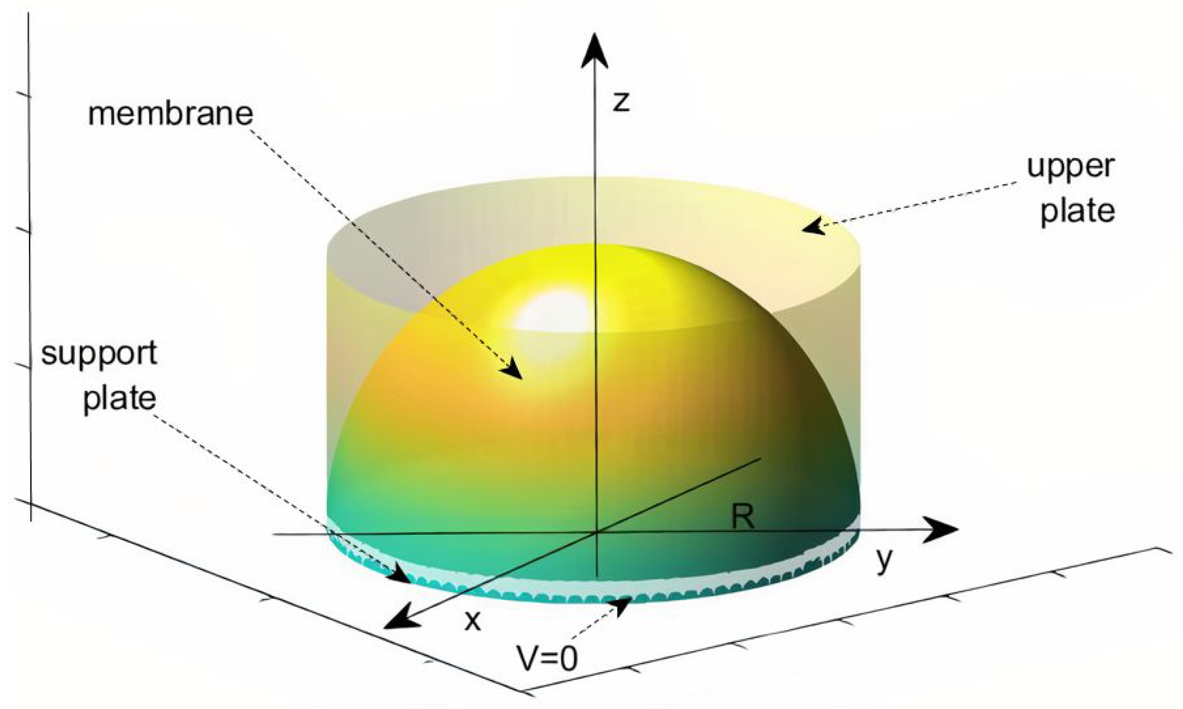
2. A Description of the 2d Electrostatic Membrane Mems Device and Previous Works

Let us consider the usual Euclidean space ${\mathbb{R}}^3$, and in it, let us consider a system of Cartesian axes $Oxyz$, where the z axis is the vertical one, as highlighted in Figure 1. The device studied in this work consists of two parallel and circular metal disks with radius R, placed at the distance d from each other. In particular, the lower disk is located on the $xy$ plane, so its center coincides with the origin of the Cartesian axis system. The device is subjected to an external electric voltage V in such a way that the lower disk is potential $V=0$. A membrane (whose radius is equal to the radius of the disks, if it is at rest), constrained to the edges of the lower disk, deforms towards the upper disk when V is applied. It is immediately apparent that the device, being circular, is endowed with radial symmetry, and therefore, by indicating the radial coordinate with r, $0<r\le R$, the profile of the membrane can only be expressed as a function of r (i.e., $u\left(r\right)$). Obviously, V must be such that it can overcome the mechanical inertia of the membrane and the corresponding value of $\mathbf{E}$ inside the device must generate the following electrostatic pressure [1,25]

$$p_{el}=\frac{1}{2}{ϵ}_0{\left|\mathbf{E}\right|}^2=\frac{1}{2}\frac{{ϵ}_0{V}^2}{{(d-u\left(r\right))}^2}$$

(1)

where ${ϵ}_0$ is the permittivity of the free space. $p_{el}$ translates into an equivalent electrostatic force $f_{el}$, as given by [1,25]

$$f_{el}=\frac{1}{2}\frac{{ϵ}_0\pi R^2{V}^2}{{(d-u\left(r\right))}^2},$$

(2)

so that a corresponding mechanical pressure p deflects the membrane towards the upper disk, obtaining a displacement in the center of the membrane, $u_0$, equal to $\frac{R^2}{4T}p$ [1,26], where T is the radial mechanical tension of the membrane. Because the membrane must not touch the upper disk for obvious electrostatic reasons, it is necessary to keep a critical security distance, $d^{*}$, such that $u\left(0\right)=u_0\le d-d^{*}$, which, in dimensionless conditions, becomes $u\left(0\right)=u_0\le 1-d^{*}$ [1,25].

Remark 1.

We highlight that $u_0$ is a crucial quantity in electrostatics, as capacitance, co-energy, electrostatic charge, electrostatic force depend on it (for detail, see [20,27]).

Historically, the first complete mathematical model of an electrostatic MEMS device was presented in [28], whose device consisted of two metal plates, one fixed and the other deformable (but anchored to the edges of a region $\mathsf{\Omega }\in {\mathbb{R}}^3$ and subject to drop voltage, which would deform the lower plate). This model, which assumed the following structure

$$\left\{\begin{array}{c}\alpha {\mathsf{\Delta }}^{2}u=\left(\beta {\int }_{\mathsf{\Omega }}{|\nabla u|}^{2}dx+\gamma \right)\mathsf{\Delta }u+\frac{{\lambda }_1{f}_1\left(x\right)}{{(1-u)}^{{\sigma }_1}\left(1+\zeta {\int }_{\mathsf{\Omega }}\frac{dx}{{(1-u)}^{{\sigma }_1-1}}\right)}\hfill \\ u=\mathsf{\Delta }u-d{u}_{\nu }=0,x\in \partial \mathsf{\Omega },d\ge 0\hfill \\ 0<u<1,x\in \mathsf{\Omega },\hfill \end{array}\right.$$

(3)

($f_1$, bounded function, depending on the dielectric properties of the material constituting the deformable plate; $\alpha$, $\beta$, $\gamma$, $\chi$, parameters that are related to the mechanical and electrical properties), although complete and exhaustive from a physical-mathematical point of view, presented certain difficulties in resolution, so that the solution was only obtainable if some simplifications were implemented [1]. Subsequently, neglecting the inertial and non-local effects, the following simplified model was obtained [28,29]:

$$\left\{\begin{array}{c}\frac{d^{2}u\left(x\right)}{d{x}^2}=-\frac{{\lambda }^2}{{(1-u\left(x\right))}^2};0\le u\left(x\right)<1;\mathrm{in}\mathsf{\Omega },\hfill \\ u=\mathsf{\Delta }u-\widehat{d}{u}_{\nu },\mathrm{on}\partial \mathsf{\Omega },\widehat{d}\ge 0.\hfill \end{array}\right.$$

(4)

(4) was studied using the Steklov boundary conditions in order to obtain Dirichlet and Navier boundary conditions when $\widehat{d}=0$ or $\widehat{d}=+\infty$. In [30], starting from (4), the following elliptical semi-linear dimensionless model for a one-dimensional (1D) membrane MEMS

$$\left\{\begin{array}{c}\frac{d^{2}u\left(x\right)}{d{x}^2}=-\frac{{\left(1+{\left(\frac{du\left(x\right)}{dx}\right)}^2\right)}^3}{\theta {\lambda }^2}{(1-u\left(x\right))}^2\mathrm{in}\mathsf{\Omega }=[-1,1]\hfill \\ 0\le u\left(x\right)<1;u=0\mathrm{on}\partial \mathsf{\Omega }\hfill \end{array}\right.$$

(5)

has been studied, where the deformable lower plate was replaced by a membrane and, moreover, $\left|\mathbf{E}\right|$ was considered to be proportional to the curvature K of the membrane [20,21,22,30,31]. In these works, the conditions of existence, uniqueness, and regularity of the solution were obtained, which allowed for the obtaining of non-ghost numerical solutions whose convergence was ensured by particular ranges of $\theta {\lambda }^2$ values [20,21,30]. We highlight that $\theta$ takes the applied voltage V into account and ${\lambda }^2$ takes the electro-mechanical properties of the material constituting the membrane into account [1]:

$${\lambda }^2=\frac{{ϵ}_0{V}^2{\left(2R\right)}^2}{2d^{3}T}.$$

(6)

From (6), ${\lambda }^2\propto V^2$, so ${\lambda }^2$ is bounded below, because a minimum value of V is required to overcome the mechanical inertia of the membrane. On the other hand, V cannot indefinitely increase, because its maximum value is fixed by the intended use of the device. Therefore, ${\lambda }^2$ is also limited by the intended use of the device.

Remark 2.

From an analytical point of view, θ has no limitations, except that it must obviously both be non-zero. However, we will see later that, numerically, the product $\theta {\lambda }^2$ will suffer specific limitations due to problems of convergence of the numerical procedures in the presence/absence of ghost solutions.

When considering a 2D circular membrane MEMS device, it follows that the profile u of the membrane only depends on the radial coordinate r, such that, only considering the radial part of the Laplace operator [31], and $\left|\mathbf{E}\right|$ in this case, is considered to be proportional to the mean curvature of the membrane (for detail, see [20]). Therefore, (4) was reformulated as follows [20]:

$$\left\{\begin{array}{c}\frac{d^{2}u\left(r\right)}{d{r}^2}=-\frac{1}{r}\frac{du\left(r\right)}{dr}-\frac{4{(1-u\left(r\right)-d^{*})}^2}{\theta {\lambda }^2}\hfill \\ u\left(R\right)=0,\frac{du\left(0\right)}{dr}=0,0<u\left(r\right)<d.\hfill \end{array}\right.$$

(7)

We note that (7), apparently, does not present the singularity, which characterizes (4). However, if in (7) we set $u\left(r\right)=1-d^{*}$, it follows that $\frac{du\left(r\right)}{dr}=0$ so that $\frac{d^{2}u\left(r\right)}{d{r}^2}=0$. But, being $\frac{d^{2}u\left(r\right)}{d{r}^2}=0=-\theta {\left|\mathbf{E}\right|}^2$, it follows that $\left|\mathbf{E}\right|=0$, and this occurrence would produce a linear deflection of the membrane that represents a physically unacceptable condition.

Remark 3.

Wrinkling is highly likely if the membrane is too thin. However, to formulate the mean curvature, it is necessary that $u\left(r\right)\in C^2\left([-L,L]\right)$, implying that abrupt local variations of the membrane profile are not allowed. Obviously, removing the hypothesis that $u\left(r\right)\in C^2\left([-L,L]\right)$ any wrinkles around the membrane can be arisen.

Model (7) has been studied both analitically and numerically, obtaining the following existence condition for the solution [20,30]

$$\theta {\lambda }^2>\frac{2R^2{d^{*}}^2}{k{ϵ}_0{V}^2}$$

(8)

in which k is the coefficient of proportionality between p and $p_{el}$. (8) ensures the absence of ghost solutions if numerical solutions that are achieved by any numerical approach exploited to recover the profile of the membrane satisfied it. It is worth noting that, from (8), the greater the external V applied the lower the value that is assigned to $\theta {\lambda }^2$ can be. Subsequently, from the equation of the model (7), $\frac{d^{2}u\left(r\right)}{d{r}^2}$ will be smaller. In other words, the higher the V, the more the membrane will be curved.

Remark 4.

We also observe that (8) ensures the existence of at least one solution for (7). However, the uniqueness of the solution is not ensured. This could create problems if the membrane deforms excessively. In this case, the risk of it touching the upper disk is high. Subsequently, the need arises to verify if the model under study admits possibly stable equilibrium positions and whether these positions are close to the upper disk. However, the numerical recovering of the membrane profile occurs for small displacements, so that the risk of the membrane touching the upper disc does not exist, as observed in Remark 6.

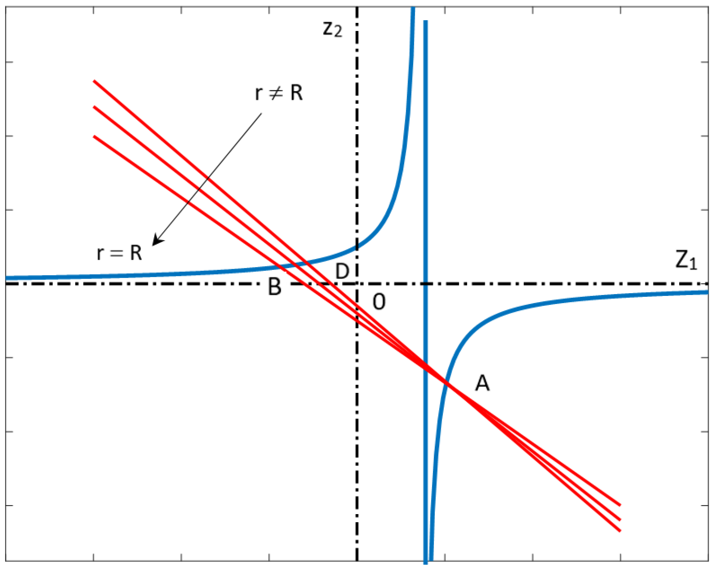
3. Critical Points and Stability

To achieve any critical points for the membrane whose profile is $u\left(r\right)$, it is necessary to transform the model (7) into the corresponding system of two ordinary differential equations of the first order in normal form [32]. In particular,

$$\left\{\begin{array}{c}\frac{d{u}_1\left(r\right)}{dr}=\overline{f}(u_1\left(r\right),u_2\left(r\right))\hfill \\ \frac{d{u}_2\left(r\right)}{dr}=\overline{g}(u_1\left(r\right),u_2\left(r\right)).\hfill \end{array}\right.$$

(9)

Therefore, to achieve any critical points, it will be sufficient to impose [32]

$$\left\{\begin{array}{c}\overline{f}(u_1\left(r\right),u_2\left(r\right))=0\hfill \\ \overline{g}(u_1\left(r\right),u_2\left(r\right))=0.\hfill \end{array}\right.$$

(10)

3.1. A More Suitable Writing of the Model under Study: Search for Critical Points

To write (7) as a system of ordinary differential equations of the first order, we consider two functions, $u_1\left(r\right)$ and $u_2\left(r\right)$, such that

$$\left\{\begin{array}{c}{u}_1\left(r\right)=u\left(r\right)\hfill \\ u_2\left(r\right)=\frac{du\left(r\right)}{dr}.\hfill \end{array}\right.$$

(11)

We immediately observe that equalities (11) can be physically investgated. In fact, $u_1\left(r\right)$ and $u_2\left(r\right)$ represent, respectively, $\forall r\in [-R,R]$, the profile of the membrane and its slope. From the physical point of view, (11) has a profound meaning, since $u_1\left(r\right)$ and $u_2\left(r\right)$ represent, locally, the position and speed of change of position of the membrane. This means that the search for equilibrium positions is entirely managed by kinematic variables.

Afterwards, (11) allows for rewriting (7) as a system of equations, where the unknown functions are, respectively, the position of the membrane and the speed of variation of the position of the membrane in the device. This permits a wide discussion about the stability of any critical points. Subsequently, when considering (11), model (7) becomes the following system, in which both $u_1\left(r\right)$ and $u_2\left(r\right)$ are two unknown functions [30]:

$$\left\{\begin{array}{c}\frac{d{u}_1\left(r\right)}{dr}=u_2\left(r\right);\hfill \\ \frac{d{u}_2\left(r\right)}{dr}=-\frac{1}{r}{u}_2\left(r\right)-\frac{4{(1-u_1\left(r\right)-d^{*})}^2}{\theta {\lambda }^2}\hfill \\ u_1\left(R\right)=0;u_2\left(0\right)=0.\hfill \end{array}\right.$$

(12)

Therefore, in this case, we can write:

$$\left\{\begin{array}{c}\overline{f}(u_1\left(r\right),u_2\left(r\right))=u_2\left(r\right)\hfill \\ \overline{g}(u_1\left(r\right),u_2\left(r\right))=-\frac{1}{r}{u}_2\left(r\right)-\frac{4{(1-u_1\left(r\right)-d^{*})}^2}{\theta {\lambda }^2}.\hfill \end{array}\right.$$

(13)

Accordingly, from (13), while taking (10) into account and considering that $\theta {\lambda }^2\ne 0$, we obtain the following critical point

$$(u_1^0,u_2^0)=(1-d^{*},0)$$

(14)

which, as proved in the following, is a stable point. It is worth noting that the only equilibrium position obtained corresponds, as reported in (14), to a profile $u\left(r\right)$ of the membrane, such that ${max}_r\left\{u\left(r\right)\right\}=1-d^{*}$. In other words, there is a point on the membrane that is very close to the upper disk whose distance is $1-d^{*}$ (for reasons of symmetry, this point can only be $u_0=u\left(0\right)$). It follows that, in the presence of any instability, the membrane could touch the upper disk with consequent generation of unwanted electrostatic discharges. Hence, it is worth studying the stability of this unique equilibrium position to understand whether there are risks in electrostatic terms.

Remark 5.

We observe that the critical point obtained in (14) is exactly equal to the critical point obtained in [24] for the same membrane MEMS device, but in 1D configuration. This important result is due to the fact that the 2D device is characterized by symmetry with respect to the vertical axis z. Therefore, whatever the plane π whose support is the vertical axis z, the intersection between π and the membrane is a curve, C, being symmetrical with respect to z. Subsequently, C, together with its vertical projection on the horizontal plane $z=0$, can be considered as a device totally similar to the device 1D studied in [24], and given the arbitrariness of π (and, therefore, C is also arbitrary), one deduces that both the 1D and 2D geometries have the same critical points.

Remark 6.

It is worth nothing that the MEMS membrane device that is studied in this work is not in the regime of large displacements. It is true that, in the paper, we show that the only equilibrium position of the membrane occurs at $1-d^{*}$, as specified in (14), but this position is entirely theoretical. In fact, as revealed by numerical simulations that were performed by both shooting techniques and by collocation methods (for details, see [30]), the reconstruction of the membrane profile in conditions of convergence of the numerical procedures and in the absence of ghost solutions has highlighted regimes of small displacements highlighting the appropriate uses of the device, for example, in the biomedical field as an intravenous drug diffuser system, where small movements of the membrane are required.

3.2. On the Stability of the Critical Point

Exploiting the first Lyapunov criterion based on the linearization of the non-linear system (12) in the neighborhood of the critical state, we can obtain information regarding the stability of the critical point [32]. Because it is easy to verify, model (12) can be rewritten in a the following general form:

$$\left\{\begin{array}{c}\frac{d{u}_1\left(r\right)}{dr}=u_2\left(r\right)=\overline{f}\left(\mathbf{u}\left(r\right)\right)\hfill \\ \frac{d{u}_2\left(r\right)}{dr}=-\frac{1}{r}{u}_2\left(r\right)-\frac{4{(1-u_1\left(r\right)-d^{*})}^2}{\theta {\lambda }^2}=\overline{g}\left(\mathbf{u}\left(r\right)\right)\hfill \end{array}\right.$$

(15)

where $\mathbf{u}\left(r\right)={\left[u_1\left(r\right)u_2\left(r\right)\right]}^T$. Therefore, setting

$$\mathbf{f}\left(\mathbf{u}\left(r\right)\right)=\left(\begin{array}{c}\overline{f}(u_1\left(r\right),u_2\left(r\right))\\ \overline{g}(u_1\left(r\right),u_2\left(r\right))\end{array}\right)=\left(\begin{array}{c}{u}_2\left(r\right)\\ -\frac{1}{r}{u}_2\left(r\right)-\frac{{(1-u_1\left(r\right)-d^{*})}^2}{\theta {\lambda }^2}\end{array}\right),$$

(16)

(12) can be matricially written, as follows:

$$\dot{\mathbf{u}}\left(r\right)=\mathbf{f}\left(\mathbf{u}\left(r\right)\right)$$

(17)

where $\dot{\mathbf{u}}\left(r\right)={\left[\frac{d{u}_1\left(r\right)}{dr}\frac{d{u}_2\left(r\right)}{dr}\right]}^T$. To linearize (17), we use the following change of variable:

$$\left\{\begin{array}{c}{u}_1\left(r\right)=u_1^0+ϵ\xi \left(r\right)\hfill \\ u_2\left(r\right)=u_2^0+ϵ\eta \left(r\right)\hfill \end{array}\right.$$

(18)

where $ϵ$ is a quantity that is small enough. Therefore, taking (18) into account and when considering that $u_1^0$ and $u_2^0$ do not depend on r, it is possible to write the folowing [32]:

$$\left\{\begin{array}{c}\frac{d{u}_1\left(r\right)}{dr}=ϵ\frac{d\xi \left(r\right)}{dr}=\overline{f}(u_1\left(r\right),u_2\left(r\right))\hfill \\ \frac{d{u}_2\left(r\right)}{dr}=ϵ\frac{d\eta \left(r\right)}{dr}=\overline{g}(u_1\left(r\right),u_2\left(r\right)).\hfill \end{array}\right.$$

(19)

From (19), developing in Taylor series both $\overline{f}(u_1\left(r\right),u_2\left(r\right))$ and $\overline{g}(u_1\left(r\right),u_2\left(r\right))$ and neglecting the terms of orders higher than the linear one, setting $\tau =\sqrt{{\xi }^2+{\eta }^2}$, it follows that

$$\left\{\begin{array}{c}ϵ\frac{d\xi \left(r\right)}{dr}=\overline{f}(u_1^0+ϵ\left(r\right),u_2^0+ϵ\eta \left(r\right))\approx \hfill \\ \approx \overline{f}(u_1^o,u_2^0)+ϵ\frac{\partial \overline{f}(u_1^0,u_2^0)}{\partial u_1}\xi \left(r\right)+ϵ\frac{\partial \overline{f}(u_1^o,u_2^0)}{\partial u_2}\eta \left(r\right)+o\left(\tau \right)\hfill \\ ϵ\frac{d\eta \left(r\right)}{dr}=\overline{g}(u_1^0+ϵ\left(r\right),u_2^0+ϵ\eta \left(r\right))\approx \hfill \\ \approx \overline{g}(u_1^o,u_2^0)+ϵ\frac{\partial \overline{g}(u_1^0,u_2^0)}{\partial u_1}\xi \left(r\right)+ϵ\frac{\partial \overline{g}(u_1^o,u_2^0)}{\partial u_2}\eta \left(r\right)+o\left(\tau \right).\hfill \end{array}\right.$$

(20)

Equations (20) make sense, as both $u_1\left(r\right)$ and $u_2\left(r\right)$ are analytical functions, as proven in [21], allowing for the linearization by means of $\frac{\partial \overline{f}(u_1^0,u_2^0)}{\partial u_1}$, $\frac{\partial \overline{f}(u_1^0,u_2^0)}{\partial u_2}$, $\frac{\partial \overline{g}(u_1^0,u_2^0)}{\partial u_1}$ and $\frac{\partial \overline{g}(u_1^0,u_2^0)}{\partial u_2}$. Moreover, observing that $\overline{f(u_1^0,u_2^0)}$ = $\overline{g(u_1^0,u_2^0)}$ = 0 and neglecting the terms of orders higher than $\tau$, we can write

$$\left\{\begin{array}{c}\frac{d\xi \left(r\right)}{dr}=\frac{\partial \overline{f}(u_1^0,u_2^0)}{\partial u_1}\xi \left(r\right)+\frac{\partial \overline{f}(u_1^0,u_2^0)}{\partial u_2}\eta \left(r\right)\hfill \\ \frac{d\eta \left(r\right)}{dr}=\frac{\partial \overline{g}(u_1^0,u_2^0)}{\partial u_1}\xi \left(r\right)+\frac{\partial \overline{g}(u_1^0,u_2^0)}{\partial u_2}\eta \left(r\right)\hfill \end{array}\right.$$

(21)

and, since $\frac{\partial \overline{f}(u_1^0,u_2^0)}{\partial u_1}=\frac{\partial \overline{g}(u_1^0,u_2^0)}{\partial u_1}=0$, $\frac{\partial \overline{f}(u_1^0,u_2^0)}{\partial u_2}=\eta \left(r\right)$, $\frac{\partial \overline{g}(u_1^0,u_2^0)}{\partial u_2}=-\frac{\eta \left(r\right)}{r}$, (21) becomes

$$\left\{\begin{array}{c}\frac{d\xi \left(r\right)}{dr}=\frac{\partial \overline{f}(u_1^0,u_2^0)}{\partial u_1}\xi \left(r\right)+\frac{\partial \overline{f}(u_1^0,u_2^0)}{\partial u_2}\eta \left(r\right)=\eta \left(r\right)\hfill \\ \frac{d\eta \left(r\right)}{dr}=\frac{\partial \overline{g}(u_1^0,u_2^0)}{\partial u_1}\xi \left(r\right)+\frac{\partial \overline{g}(u_1^0,u_2^0)}{\partial u_2}\eta \left(r\right)=-\frac{\eta \left(r\right)}{r}\hfill \end{array}\right.$$

(22)

from which

$$\xi \left(r\right)+ln\eta \left(r\right)=A$$

(23)

with A constant.

Remark 7.

Matricially, system (21) (i.e., the linearized version of the non-linear system (17) around the critical point) can be written, as follows:

$$\dot{\mathbf{z}}=A\mathbf{z}$$

(24)

where

$$\mathbf{z}=\left(\begin{array}{c}\xi \left(r\right)\\ \eta \left(r\right)\end{array}\right);\dot{\mathbf{z}}=\left(\begin{array}{c}\frac{d\xi \left(r\right)}{dr}\\ \frac{d\eta \left(r\right)}{dr}\end{array}\right);A=\left(\begin{array}{cc}\frac{\partial \overline{f}(u_1^0,u_2^0)}{\partial u_1}& \frac{\partial \overline{f}(u_1^0,u_2^0)}{\partial u_2}\\ \frac{\partial \overline{g}(u_1^0,u_2^0)}{\partial u_1}& \frac{\partial \overline{g}(u_1^0,u_2^0)}{\partial u_2}\end{array}\right)=\left(\begin{array}{cc}0& 1\\ 0& -\frac{1}{r}\end{array}\right).$$

(25)

To study the stability of (24), let us introduce the following definition [33].

Definition 1

(Algebraic/geometric multiplicities of an eigenvalue). Given a square matrix A of order n, suppose that it has $r\le n$ distinct eigenvalues ${\lambda }_1,{\lambda }_2,\dots ,{\lambda }_r$ with ${\lambda }_i\le {\lambda }_j$ for $i\le j$. Therefore, the characteristic polynomial of A can be written as $P\left(s\right)={(s-{\lambda }_1)}^{{\nu }_1}{(s-{\lambda }_2)}^{{\nu }_2}...{(s-{\lambda }_r)}^{{\nu }_r}$, with ${\sum }_{i=1}{\nu }^r=n$, where ${\nu }_i\in {\mathbb{N}}^{+}$ defines the algebraic multiplicity of the generic eigenvalue ${\lambda }_i$. Moreover, the geometric multiplicity of the eigenvalue ${\lambda }_i$ is defined as the number ${\mu }_i$ of linearly independent eigenvectors that correspond to it [32].

The following result evaluates the stability of (24) while using a criterion based on the eigenvalues of the matrix A [32].

Theorem 1.

System (24) admits stable equilibrium position only if matrix A does not have eigenvalues with positive real part and if any eigenvalues with real part zero have unit index. In addition, if ${\mathbf{z}}_0={\left[z_{0,1}{z}_{0,2}\right]}^T$, then

$$\mathbf{z}\left(r\right)=e^{Ar}\mathbf{z}\left(0\right)=e^{Ar}{\mathbf{z}}_0$$

(26)

where $\mathbf{z}\left(r\right)={\left[z_1\left(r\right)z_2\left(r\right)\right]}^T$.

Remark 8.

$\left|A\right|=0$, so that at least one eigenvalue is zero [33]. This means that the origin is not an isolated equilibrium point: there is at least one line of equilibrium points or even a plane of equilibrium points [32,33]. In other words, the only critical point obtained is represented by (14), where $d^{*}$ is the critical security distance. Accordingly, as the variation of $d^{*}$ changes the equilibrium point, in theory, we have infinite equilibrium points obtained $\forall d^{*}\in [0,1]$.

Moreover, because that the eigenvalues of matrix A are

$${\lambda }_1=0;{\lambda }_2=-\frac{1}{r}<0,$$

(27)

by Theorem 1, it follows that (24) admits stable equilibrium position.

Remark 9.

Because the number of eigenvalues of A counted with their algebraic multiplicity is equal to the order of A and the geometric multiplicity of each eigenvalue coincides with the algebraic multiplicity, then A is diagonalizable [32,33].

Therefore, exploiting Remark 9 and taking into account both (27), $e^{Ar}$ can be written as [33] $e^{Ar}={\sum }_{k=1}^n{\mathbf{t}}_k·{\mathbf{s}}_k{e}^{{\lambda }_{k}r}={\mathbf{t}}_1·{\mathbf{s}}_1+{\mathbf{t}}_2·{\mathbf{s}}_2{e}^{-1}$, where ${\mathbf{t}}_k$ and ${\mathbf{s}}_k$ are the left and right eigenvectors that correspond to ${\lambda }_k$, respectively. Subsequently, we can easily get that ${\mathbf{t}}_1={\left[10\right]}^T$, ${\mathbf{t}}_2={[1-r^{-1}]}^T$, ${\mathbf{s}}_1=\left[1r\right]$, ${\mathbf{s}}_2=\left[01\right]$, so that

$$e^{Ar}=\left(\begin{array}{cc}\frac{1}{r}& r+e^{-1}\\ 0& -\frac{e^{-1}}{r}\end{array}\right)$$

(28)

is limited in norm (for $r\ne 0$) and (26) can be written, as follows:

$$\left\{\begin{array}{c}{z}_1\left(r\right)=\frac{z_{0,1}}{r}+(r+e^{-1})z_{0,2}\hfill \\ z_2\left(r\right)=-\frac{z_{0,2}{e}^{-1}}{r}.\hfill \end{array}\right.$$

(29)

From (29), eliminating the parameter r, we easily obtain

$$z_1\left(r\right)z_2\left(r\right)=-\frac{z_{0,1}e{z}_2^2\left(r\right)}{z_{0,2}}-\frac{z_{0,2}^2}{e}+\frac{z_{0,2}}{e}{z}_2\left(r\right).$$

(30)

(30) represents a curve that can be written as

$$z_1\left(r\right)z_2\left(r\right)=\overline{A}{z}_2^2\left(r\right)+\overline{B}+\overline{C}{z}_2\left(r\right)$$

(31)

where $\overline{A}=-\frac{z_{0,1}e}{z_{0,2}}$, $\overline{B}=-\frac{z_{0,2}^2}{e}$ and $\overline{C}=\frac{z_{0,2}}{e}$. To study the curve (31), one needs to evaluate the determinants of the following matrices:

$$H=\left(\begin{array}{ccc}\overline{A}& -\frac{1}{2}& 1\\ -\frac{1}{2}& 0& 0\\ 1& 0& \overline{B}\end{array}\right);H_1=\left(\begin{array}{cc}\overline{A}& -\frac{1}{2}\\ -\frac{1}{2}& 0\end{array}\right).$$

(32)

In particular, with $\left|H\right|\ne 0$ and $|H_1|<0$, (31) represents an equilateral hyperbola, as shown in Figure 2 (blue lines). Moreover, from (29), we can also write

$$z_2\left(r\right)=-\frac{z_1\left(r\right)}{r(er+1)}+\frac{z_{0,1}}{r^2(er+1)}$$

(33)

that are straight lines passing for a fixed point (point A in Figure 2), as $r\to R$. Afterwards, as r increases (obviously excluding $r=0$ as a singular value), the hyperbola is traversed such that the point D in the Figure 2 (when $r\ne R$) tends to the point B (when $r=R$).

On the Stability of the Starting Non-Linear System

To study the stability for (17), let us introduce the following Lemma [32].

Lemma 1.

Let us consider a non-linear system $\dot{\mathbf{u}}\left(r\right)=\mathbf{f}\left(\mathbf{u}\left(r\right)\right)$ and its linearized system $\dot{\mathbf{z}}=A\mathbf{z}$. If $\dot{\mathbf{z}}=A\mathbf{z}$ is stable, then $\dot{\mathbf{u}}\left(r\right)=\mathbf{f}\left(\mathbf{u}\left(r\right)\right)$ is also stable.

Now, we are ready to introduce the following result.

Proposition 1.

The critical point (14) is a stable equilibrium point for the linear system (17).

Proof. 

See Appendix A.1 □

$(u_1^0,u_2^0)=(1-d^{*},0)$, even if it identifies a point that is very close to the upper disk of the device (for which there is a real risk that the membrane touches the upper disk), is nevertheless of stable equilibrium, as, electrostatically, taking into account that ${(1-u\left(r\right))}^{-2}\approx {\left(d^{*}\right)}^{-1}$, from (1), we can write

$$p_{el}=\frac{1}{2}\frac{{ϵ}_0{V}^2}{{(1-u\left(r\right))}^2}\approx \frac{{ϵ}_0{V}^2}{2d^{*}},$$

(34)

thereby fixing V, $p_{el}$ does not fluctuate. Thus, with the mechanical pressure p in the device proportional to $p_{el}$, p also does not fluctuate. Finally, from (34), since $p_{el}$ is constant, $u\left(r\right)$ also does not modify, so that the profile of the membrane is stable.

Remark 10.

As highlighted above, the only equilibrium position (14) is stable, unlike that obtained for 1D geometry where the same equilibrium position was found to be unstable (see [24]). This is due to the fact that, in 2D geometry, the symmetry of the device with respect to the vertical axis z imposes a sort of stability of the position of the membrane, both at rest and during deformation. This was also confirmed by the numerical simulations in which the recovering of the membrane profile markedly highlighted the phenomenon of stability (for detail, see [24]). On the other hand, in 1D geometry, the same numerical techniques showed a marked instability when the membrane reached the equilibrium configuration (for detail, see [23]).

Remark 11.

The phenomenon of the transition between the stability and instability of an equilibrium in a MEMS device membrane can have multiple causes. For example, instability phenomena can occur when the non-equilibrium state is related to the restriction failure mode occurring in the operation of MEMS devices. From the electrostatic point of view, membrane instability can be determined by small perturbations of the $p_{el}$ distribution in the device influencing: (i) the equilibrium path; (ii) the number and unstable positions; and, (iii) the behavior of the membrane in post-equilibrium conditions. Moreover, $p_{el}$, as specified in (34), depends on V. In addition, snapping behavior could occur if the device is repeatedly loaded and unloaded electrically. Finally, evident phenomena of instability could occur due to the Casimiro effect, regardless of the V applied.

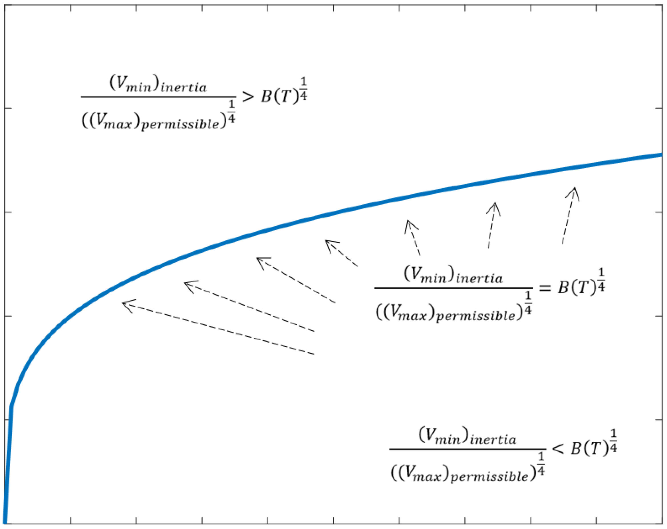
4. Voltage V and Its Admissible Values

4.1. $V_{Min}$ to Win the Mechanical Inertia of the Membrane

Proposition 2.

Let us consider the two-dimensional (2D) membrane MEMS device whose analytical model is (7). If the condition of existence (8) holds, then the minimum V that is needed to win the membrane mechanical inertia, ${\left(V_{min}\right)}_{inertia}$, verifies the following inequality:

$${\left(V_{min}\right)}_{inertia}=\sqrt[4]{\frac{d^3{d^{*}}^{2}T}{{ϵ}_0^2\theta k}}.$$

(35)

Proof. 

See Appendix A.2 □

(35) has a very important physical significance. In fact, once the geometry of the device is fixed (i.e., d fixed), materials with high mechanical stresses (i.e., high values of T) require high values of V to deform the membrane towards the upper disk, so that intended uses of the device requiring low external V cannot be considered. It follows that MEMS device membranes with high T values can be used in electrical devices for industrial applications, where the operating V is not negligible.

Remark 12.

${\left(V_{min}\right)}_{inertia}$, as highlighted in (35), depends on d, T, $d^{*}$, ${ϵ}_0$ and θ. This result is similar to that obtained in 1D geometry (see [22,24]). However, in the latter case, ${\left(V_{min}\right)}_{inertia}$ also depends on the sixth power of parameter $H=sup\left\{u^{\prime }\right\}=99$ by forcing ${\left(V_{min}\right)}_{inertia}$ to assume considerably higher values than in the case 2D studied here. In other words, in 2D geometry, reduced values of V are sufficient for moving the membrane as compared to the 1D case, thus allowing the device to also be used in biomedical applications, where V, usually, assumes extremely contained values.

4.2. The Maximum Value of V, ${\left(V_{Max}\right)}_{Permissible}$, in Order That the Membrane Does Not Touch the Upper Disk

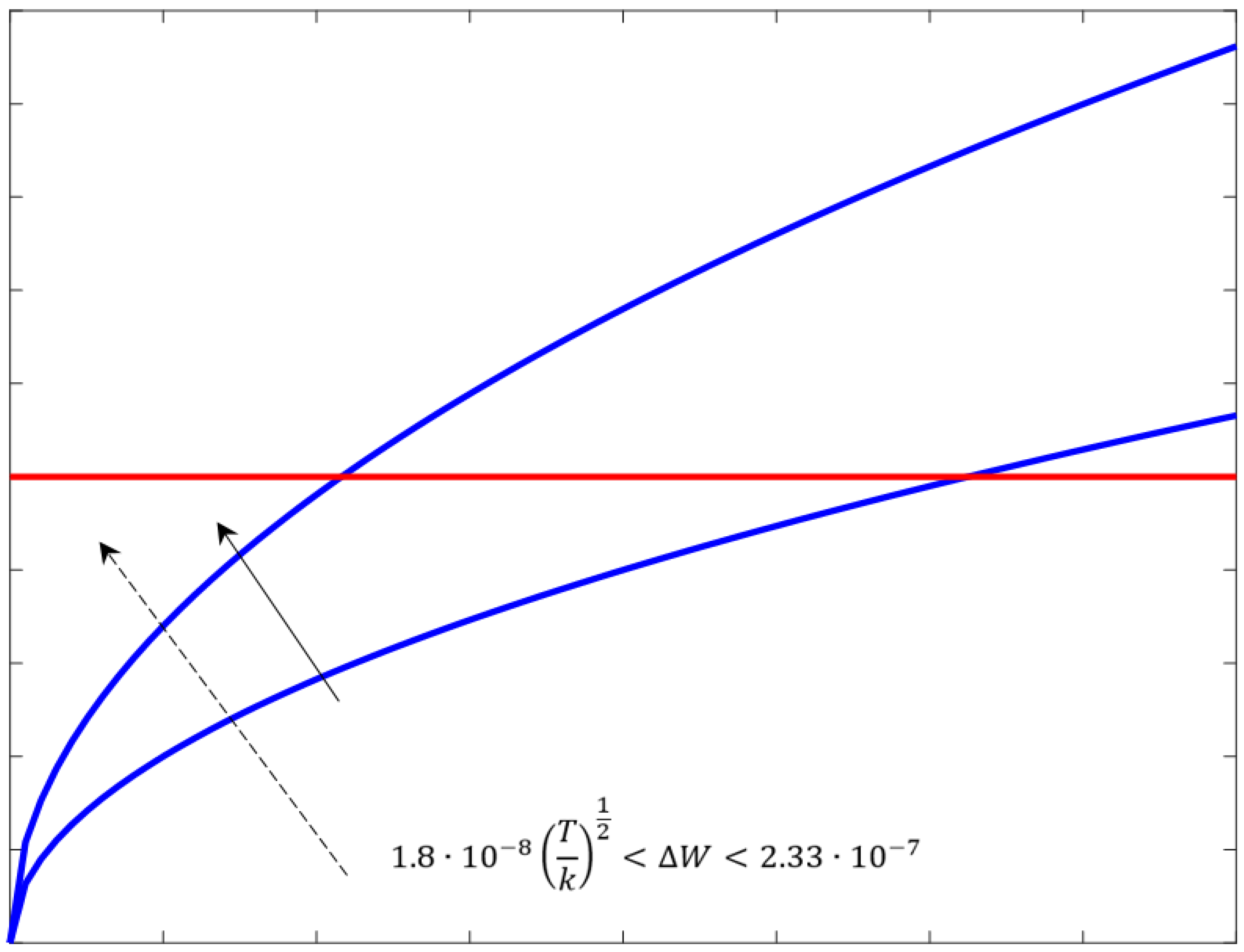
For this purpose, here we present some useful propositions [20].

Proposition 3.

If $u_0$ is the deflection in the center of the membrane (i.e., $u_0=u\left(0\right)$), the following inequality holds:

$$u_0\le \frac{k{ϵ}_0{V}^2}{2d^{*}}.$$

(36)

Proof. 

See Appendix A.3. □

(36) has an important physical significance. In fact, as V increases, the deflection in the center of the membrane, $u_0$, increases. However, $u_0$ does not increase indefinitely, as the presence of $d^{*}$ in (36) limits its value, avoiding the risk of the membrane touching the upper disk.

Remark 13.

It is worth noting that (36) is completely overlapping with the inequality obtained for $u_0$ in 1D geometry (see [24]). This is due to the fact that the MEMS membrane device that is studied in this paper is symmetrical with respect to the vertical axis z. Accordingly, as highlighted in Remark 5, each C curve belonging to π represents a good approximation of the membrane in a device in 1D gemetry.

The following Proposition has a mere mathematical meaning and it will be used in the following to demonstrate some relevant statements for the MEMS membrane device under study.

Proposition 4.

For the 2D membrane MEMS under study, $\sqrt{k}$ is computable, as follows:

$$\sqrt{k}=\frac{\sqrt{p}}{2\sqrt{p_{el}}}$$

(37)

Proof. 

See Appendix A.4. □

Proposition 5.

For the 2D membrane MEMS under study, the following inequality holds:

$$\frac{k{ϵ}_0{V}^2}{2d^{*}}<1-d^{*}.$$

(38)

Proof. 

See Appendix A.5. □

(38) looks physically interesting. In fact, it can be written, as follows:

$$\underset{f\left(V\right)}{\underbrace{k{ϵ}_0{V}^2}}<\underset{g\left(d^{*}\right)}{\underbrace{2(1-d^{*})d^{*}}}$$

(39)

from which it can be deduced that the chosen safety distance governs the intended use of the device.

Propositions 3, 4, and 5 have been introduced and proved, so that we are now able to compute the ${\left(V_{max}\right)}_{permissible}$.

Proposition 6.

For the 2D membrane MEMS device under study, it follows that

$${\left(V_{max}\right)}_{permissible}<\sqrt{\frac{2(1-d^{*})d^{*}}{k{ϵ}_0}}.$$

(40)

Proof. 

See Appendix A.6. □

It is very significant that ${\left(V_{max}\right)}_{permissible}$, according to (40), exclusively depends on the safety distance chosen. Furthermore, k appearing in the denominator of the right side of the inequality imposes that high $p_{el}$ allow ${\left(V_{max}\right)}_{permissible}$, allowing for the use of the device in industrial applications in which V is remarkable.

Remark 14.

(40) represents the limitation of ${\left(V_{max}\right)}_{permissible}$. Its structure is quite similar to that obtained in 1D geometry (see [2,21]). However, in the latter case, $H^2$ is present in the right side of the inequality allowing, in 1D geometry, values of ${\left(V_{max}\right)}_{permissible}$ higher than in the case 2D with a consequent increase of the risk that the membrane touches the upper disk. Hence, the result obtained in this paper cautions us of this risk by highlighting that, in 2D geometry, the values attributable to ${\left(V_{max}\right)}_{permissible}$ do not allow the membrane to touch the upper disk.

The following Proposition has a mere mathematical meaning, and it will be used to prove some relevant statements.

Proposition 7.

For the 2D membrane MEMS device under study, the following condition holds:

$$\sqrt{R\theta }=\frac{R}{d}\sqrt{\frac{{ϵ}_{0}R}{2dT}}.$$

(41)

Proof. 

See Appendix A.7. □

It is worth noting that, by increasing T in (41), the value of $\theta$ decreases and, from the differential Equation (7), we have confirmation that the membrane bends to a lesser extent.

Remark 15.

(41) offers an interesting link between the parameter θ and the geometric parameters R and d and the mechanical tension T of the membrane. In fact, it is observed that the more rigid the membrane is (i.e., high values of T), the lower the values of θ, i.e., the membrane will be less sensitive to electrostatic stresses. This result is similar to that obtained in 1D geometry, as discussed in [23,24].

The following Proposition verifies a useful inequality in the continuation of the work.

Proposition 8.

For the 2D membrane MEMS device under study, the following inequality holds:

$$\sqrt[4]{\frac{d^3{d^{*}}^{2}T}{4{ϵ}_0^2\theta k}}<\sqrt{\frac{2(1-d^{*})d^{*}}{k{ϵ}_0}}$$

(42)

Proof. 

See Appendix A.8. □

After having verified the inequality (42), we are able to provide the range of feasible values for V, as stated by the following Proposition.

Proposition 9.

For the 2D membrane MEMS device under study, the range of admissible values for V is as follows:

$$\sqrt[4]{\frac{d^3{d^{*}}^{2}T}{4{ϵ}_0^2\theta k}}<V<\sqrt{\frac{2(1-d^{*})d^{*}}{k{ϵ}_0}}.$$

(43)

Proof. 

See Appendix A.9. □

Remark 16.

The result that is highlighted by (43) is similar to that obtained in 1D geometry (see [24]. In this latter case, instead of the quantity $\sqrt[4]{\frac{d^3{d^{*}}^{2}T}{4{ϵ}_0^2\theta k}}$ at the left side of the (43) compares

$$\sqrt[4]{\frac{d^3{d^{*}}^{2}T}{4{ϵ}_0^2\theta k}}\sqrt{\frac{1+H^6}{H}}.$$

(44)

Afterwards, in 1D geometry, the range of admissible values for V is considerably smaller than in the 2D case studied in this paper due to the presence of the factor $\sqrt{\frac{1+H^6}{H}}$, which makes the minimum allowable value for V much higher than in the 2 D case.

It is worth noting that, when analyzing the (43), T affects the minimum value for V. This makes sense, because T, as is known, influences the mechanical inertia of the membrane that must be overcome when V reaches its minimum value, ${\left(V_{min}\right)}_{inertia}$. On the other hand, the maximum value, ${\left(V_{max}\right)}_{permissible}$, to be assigned to V cannot disregard $d^{*}$, because it must be ensured that the membrane does not touch the upper disk. Therefore, it is clear to wonder what is the link between ${\left(V_{min}\right)}_{inertia}$ and ${\left(V_{max}\right)}_{permissible}$. The following subsection will provide the answer.

4.3. ${\left(V_{Min}\right)}_{Inertia}$ & ${\left(V_{Max}\right)}_{Permissible}$: An Interesting Relationship

Proposition 10.

For the 2D membrane MEMS device under study, the relationship between ${\left(V_{min}\right)}_{inertia}$ and ${\left(V_{max}\right)}_{permissible}$ can be written, as follows:

$${\left(V_{min}\right)}_{inertia}>\sqrt[4]{\frac{d^4}{2(10-d)\theta }}\sqrt{{\left(V_{max}\right)}_{permissible}}\sqrt[4]{T}.$$

(45)

Proof. 

See Appendix A.10. □

Remark 17.

The link between ${\left(V_{min}\right)}_{inertia}$ and ${\left(V_{max}\right)}_{permissible}$ that is governed by (45) has the same algebraic structure as the link in 1D geometry (for details, see [24,30]). However, in the latter case, there is once again the presence of $\sqrt{\frac{1+H^6}{H}}$ on the right side of the inequality, which forces ${\left(V_{min}\right)}_{inertia}$ to level up. In other words, in 1D geometry a higher voltage V is needed to overcome the mechanical inertia of the membrane.

For the usual values $d={10}^{-9}$, $\theta \approx 1$, $T=1000$ $\mathrm{Pa}$, the inequality (45) becomes

$${\left(V_{min}\right)}_{inertia}>Z\sqrt{{\left(V_{max}\right)}_{permissible}}$$

(46)

with $Z\ll 1$. Afterwards, ${\left(V_{min}\right)}_{inertia}\ll {\left(V_{max}\right)}_{permissible}$, so that (45) makes physical sense. Furthermore, (45) can be physically interpreted. In particular, in it,

$$B=\sqrt[4]{\frac{d^4}{2(10-d)\theta }}$$

(47)

is a constant, so that we can write it as follows

$$\frac{{\left(V_{min}\right)}_{inertia}}{\sqrt{{\left(V_{max}\right)}_{permissible}}}>B\sqrt[4]{T}.$$

(48)

Therefore, once the material constituting the membrane has been chosen (i.e., T has been fixed), $\frac{{\left(V_{min}\right)}_{inertia}}{\sqrt{{\left(V_{max}\right)}_{permissible}}}$ depends on B (a quantity changing with d, which depends on the geometry of the device). On the other hand, if d is fixed (i.e., B has been chosen depending on the geometry of the device), the material constituting the membrane (i.e., T) determines $\frac{{\left(V_{min}\right)}_{inertia}}{\sqrt{{\left(V_{max}\right)}_{permissible}}}$. Figure 3 shows the curve $\frac{{\left(V_{min}\right)}_{inertia}}{\sqrt{{\left(V_{max}\right)}_{permissible}}}=B\sqrt[4]{T}$, above which the area where the link between ${\left(V_{min}\right)}_{inertia}$ and ${\left(V_{max}\right)}_{permissible}$ exists.

Remark 18.

From the electrostatic point of view, when the membrane is at rest, the device has a quantity of potential energy, which, during the deformation of the membrane, varies considerably. Then, a potential energy variation $\mathsf{\Delta }W$ occurs in the device. Accordingly, it makes sense to ask whether $\mathsf{\Delta }W$ admits limitations as the membrane undergoes deformation. The next section will provide those answers.

5. Some Optimal Control Conditions

If the membrane of the device is at rest, then the distance between the membrane and the upper disk is d. Therefore, the electrostatic capacitance of the device is $C={ϵ}_0\frac{\pi R^2}{d}$, so that the potential energy of the device can be evaluated as

$$W_{initial}=\frac{1}{2}C{V}^2=\frac{{ϵ}_0\pi R^2{V}^2}{2d}.$$

(49)

If the membrane deforms, $C={ϵ}_0{\int }_0^{\pi }Z\left(\varphi \right){\int }_{-R}^R\frac{dr}{d-u\left(r\right)}d\varphi$, and the final potential energy becomes

$$W_{final}=\frac{1}{2}{ϵ}_0{V}^2{\int }_0^{\pi }Z\left(\varphi \right){\int }_{-R}^R\frac{dr}{d-u\left(r\right)}d\varphi ,$$

(50)

where $Z\left(\varphi \right)$ is a bounded and continuous function, depending on $\varphi$. Therefore, the total variation of the potential energy, $\mathsf{\Delta }W=W_{final}-W_{initial}$, becomes

$$\begin{array}{c}\hfill \mathsf{\Delta }W=\frac{1}{2}{ϵ}_0{V}^2\left\{{\int }_0^{\pi }Z\left(\varphi \right){\int }_{-R}^R\frac{dr}{d-u\left(r\right)}d\varphi -\frac{\pi R^2}{d}\right\}.\end{array}$$

(51)

In addition, observing that $d-u\left(r\right)\ge d-d^{*}$, we can write $\frac{1}{d-u\left(r\right)}\le \frac{1}{d-d^{*}}$, so that (51) becomes

$$\mathsf{\Delta }W\le \frac{1}{2}{ϵ}_0{V}^2\left\{\frac{2R}{d-d^{*}}{\int }_0^{\pi }Z\left(\varphi \right)d\varphi -\frac{\pi R^2}{d}\right\}.$$

(52)

$Z\left(\varphi \right)$ being a bounded and continuous function, it follows that ${\int }_0^{\pi }Z\left(\varphi \right)d\varphi \le D$, where D is a positive constant. Subsequently, (52) can be written as

$$\mathsf{\Delta }W\le \frac{1}{2}{ϵ}_0{V}^2\left\{\frac{2RD}{d-d^{*}}-\frac{\pi R^2}{d}\right\}.$$

(53)

From (43), we can write $\sqrt{\frac{d^3{d^{*}}^{2}T}{4{ϵ}_0^2\theta k}}<V^2<\frac{2(1-d^{*})d^{*}}{k{ϵ}_0}$ so that, while taking (53) into account, it easily follows that

$$\mathsf{\Delta }W<\frac{(1-d^{*})d^{*}}{k}\left\{\frac{2RD}{d-d^{*}}-\frac{\pi R^2}{d}\right\}.$$

(54)

Conversely, from condition (35), $V^2>{\left(V_{min}\right)}_{inertia}^2=\sqrt{\frac{d^3{d}^{*}T}{4{ϵ}_0^2\theta k}}$, from which

$$\mathsf{\Delta }W>\frac{1}{2}{ϵ}_0\left\{\frac{2RD}{d-d^{*}}-\frac{\pi R^2}{d}\right\}{V}^2>\frac{1}{2}{ϵ}_0\left\{\frac{2RD}{d-d^{*}}-\frac{\pi R^2}{d}\right\}\sqrt{\frac{d^3{d}^{*}T}{4{ϵ}_0^2\theta k}}.$$

(55)

Finally, combining (54) and (55), we easily obtain the range of the admissible values for $\mathsf{\Delta }W$:

$$\frac{1}{2}\sqrt{\frac{d^3{d}^{*}}{4}}\frac{\sqrt{T}}{\sqrt{k}\sqrt{\theta }}<\mathsf{\Delta }W<\frac{(1-d^{*})d^{*}}{k}\left\{\frac{2RD}{d-d^{*}}-\frac{\pi R^2}{d}\right\}$$

(56)

from which, with the usual values for the parameters, we achieve $1.8·{10}^{-8}\frac{\sqrt{T}}{\sqrt{k}}<\mathsf{\Delta }W<2.33·{10}^{-7}$. Figure 4 shows the area of possible values for $\mathsf{\Delta }W$, which corresponds to the area that is bounded above by the red straight line, while it is bounded below by the less concave blue curve. Obviously, this area shrinks as k increases. It is worth noting that, from an energy point of view, the fact that the area of possible values is limited (as shown in Figure 4) guarantees us that the membrane MEMS device under study is subject to variations in potential energy of limited amplitude reducing the risk of any damage. However, as seen above, $\mathsf{\Delta }W$ strictly depends on V and V is closely related to $\left|\mathbf{E}\right|$. Therefore, it is imperative to know the values of V and $\left|\mathbf{E}\right|$ maximizing $\mathsf{\Delta }W$. The following Subsections answer this question.

Remark 19.

The range of admissible values for $\mathsf{\Delta }W$ in 1D geometry assumed the form [24]:

$$\frac{8d^{*}T{d}^3(1-d^{*})}{d(d-d^{*})\theta }\frac{1+H^6}{H}<\mathsf{\Delta }W<\frac{2{\left(d^{*}\right)}^2(1-d^{*})L}{kd(d-d^{*})}$$

(57)

where L is the length of the device. Additionally, for the range of values for $\mathsf{\Delta }W$ in 1D geometry appears $\frac{1+H^6}{H}$, which considerably reduces the range of admissible values. In particular, it is deduced that, in 1D geometry, higher energy levels are required to overcome the mechanical inertia of the membrane due to the presence of $\frac{1+H^6}{H}$ in (57), unlike the 2 D device studied in this paper, åwhere the absence of $\frac{1+H^6}{H}$ in (56) allows overcoming the inertia of the membrane through lower energy contents.

5.1. About the Values of V Maximizing $\mathsf{\Delta }W$.

As known (see (A1)), $u\left(r\right)\le \frac{k{ϵ}_0{V}^2}{2d^{*}}\left\{1-{\left(\frac{r}{R}\right)}^2\right\}$, so that

$$d-u\left(r\right)\ge d-\frac{k{ϵ}_0{V}^2}{2d^{*}}\left\{1-{\left(\frac{r}{R}\right)}^3\right\}>\frac{2d{d}^{*}-k{ϵ}_0{V}^2}{2d^{*}}$$

(58)

from which

$$\frac{1}{d-u\left(r\right)}<\frac{2d^{*}}{2d{d}^{*}-k{ϵ}_0{V}^2},$$

(59)

with $2d{d}^{*}-k{ϵ}_0{V}^2\ne 0$. As previously calculated, $C={ϵ}_0{\int }_0^{\pi }Z\left(\varphi \right){\int }_{-R}^R\frac{dr}{d-u\left(r\right)}d\varphi$ that, while taking the inequality (59) into account, becomes $C<\frac{4{ϵ}_{0}D{d}^{*}R}{2d{d}^{*}-k{ϵ}_0{V}^2}$. Therefore, from (52), we can write

$$\mathsf{\Delta }W=W_{final}-W_{initial}<\underset{h\left(V\right)}{\underbrace{\frac{2{ϵ}_0^{2}D{d}^{*}R{V}^2}{2d{d}^{*}-k{ϵ}_0{V}^2}-\frac{{ϵ}_0\pi R^2{V}^2}{2d}}}$$

(60)

where $h\left(V\right)$ is positively defined, so that the only stationary value for $h\left(V\right)$ is

$$V^{*}=\sqrt{\frac{2\pi R^{2}d{d}^{*}-8{ϵ}_{0}D{d}^{*}2}{k{ϵ}_0\pi R^2}}.$$

(61)

Moreover, it is easy to verify that $V^{*}$ is a point of maximum for $h\left(V\right)$ (we discard the negative root, as this value of V would deform the membrane symmetrically with respect to the lower disk, i.e., the condition is physically impossible to obtain). In addition, it is also easy to verify that $V^{*}>{\left(V_{min}\right)}_{inertia}$. $d^{*}$ plays a fundamental role in the formulation of $V^{*}$, as seen in (61). This is due to the fact that $V^{*}$, being the electrical voltage value that maximizes $\mathsf{\Delta }W$, would allow, at least theoretically, that the membrane deforms until, for $r=0$, $u\left(r\right)=1-d^{*}$.

5.2. A Useful Limitation for $\mathsf{\Delta }W$ Achieved Starting from $\left|\mathbf{E}\right|$

Starting from (4) and (7), and taking into account (A18), it follows that

$${\left|\mathbf{E}\right|}^2=\frac{1}{r\theta }\frac{du\left(r\right)}{dr}+\frac{{(1-u\left(r\right)-d^{*})}^2}{{\theta }^2{\lambda }^2}.$$

(62)

Being $W_{final}=0.5{ϵ}_0{\left|\mathbf{E}\right|}^2$, it makes sense to write

$$\mathsf{\Delta }W=\frac{1}{2}{ϵ}_0\left\{\frac{1}{r\theta }\frac{du\left(r\right)}{dr}+\frac{{(1-u\left(r\right)-d^{*})}^2}{{\theta }^2{\lambda }^2}\right\}-\frac{{ϵ}_0\pi R^2{V}^2}{2d}$$

(63)

and taking into account that $1-u-d^{*}<1-d^{*}$ and $\frac{du\left(r\right)}{dr}<\overline{H}$, with $\overline{H}=99$ positive constant (see [21]), equality (63) becomes

$$\mathsf{\Delta }W<\frac{1}{2}{ϵ}_0\left\{\frac{1}{r\theta }\overline{H}+\frac{{(1-d^{*})}^2}{{\theta }^2{\lambda }^2}\right\}-\frac{{ϵ}_0\pi R^2{V}^2}{2d}.$$

(64)

Proposition 11.

When considering both (53) and (64), it follows that

$$\frac{1}{2}{ϵ}_0{V}^2\left\{\frac{2RD}{d-d^{*}}-\frac{\pi R^2}{d}\right\}<\frac{1}{2}{ϵ}_0\left\{\frac{1}{r\theta }\overline{H}+\frac{{(1-d^{*})}^2}{{\theta }^2{\lambda }^2}\right\}-\frac{{ϵ}_0\pi R^2{V}^2}{2d}$$

(65)

Proof. 

See Appendix A.11. □

Afterwards, by Proposition 11, we can easily write

$$\mathsf{\Delta }W<\frac{1}{2}{ϵ}_0\left\{\frac{1}{r\theta }\overline{H}+\frac{{(1-d^{*})}^2}{{\theta }^2{\lambda }^2}\right\}-\frac{{ϵ}_0\pi R^2{V}^2}{2d},$$

(66)

which represent the limitation for $\mathsf{\Delta }W$ (depending on $\theta$), achieved starting from $\left|\mathbf{E}\right|$. It is worth nothing that the limitation (66) is oversized, because $\overline{H}=99$ was obtained in [21] by means of a sequence of inequalities. However, even if the value 99 is high, it is analytically correct.

Remark 20.(66) can be considered to be analogous to the limitation

$$\mathsf{\Delta }W<\frac{{ϵ}_0}{2{\theta }^2{\lambda }^2}{(1+H^2)}^3{(1-d^{*})}^2-{ϵ}_{0}L\frac{V^2}{L}$$

(67)

achieved in 1D geometry (for details, see [24,30]. However, the presence of ${(1+H^2)}^3$ in (67) raises the permissible energy levels in 1D geometry with the risk of the membrane touching the upper disk.).

6. Conclusions and Perspectives

The starting point of this paper concerns the study of the stability of the critical configurations of a second-order nonlinear boundary value problem with singularity relating to a 2D circular electostatic membrane MEMS with radial symmetry. In the model, because $\mathbf{E}$ is locally orthogonal to the straight line tangent to the membrane, it makes sense to consider $\left|\mathbf{E}\right|$ proportional to the mean curvature of the membrane at the same point. A single critical point is obtained, corresponding to the position of the membrane, where its central point reaches the maximum height allowed. Using the first Lyapunov criterion, it is verified that the only equilibrium position obtained is also stable. Furthermore, because the device is subjected to an external voltage V, both its minimum value capable of overcoming the mechanical inertia of the membrane, ${\left(V_{min}\right)}_{inertia}$, and its maximum allowed value, ${\left(V_{max}\right)}_{permissible}$, are obtained in order to determine an operating range of possible values for V. Thus, the solution of the inverse problem in the MEMS device under study has been addressed: starting from the deformation of the membrane, the range of allowed values of V was evaluated. Furthermore, the bond obtained between ${\left(V_{min}\right)}_{inertia}$ and ${\left(V_{max}\right)}_{admissible}$ explicitly depends on the value of the mechanical tension T to which the membrane was subjected. Accordingly, once we have chosen the material that constitutes the membrane (i.e., once T has been set), we obtain an easy and operational $\frac{{\left(V_{min}\right)}_{inertia}}{{\left(V_{max}\right)}_{admitted}}$. It is worth noting that the sophisticated mathematical models describing the phenomena involved in detail are obviously complex and do not allow easy study. Therefore, some simplifications in the geometry of the device have proven to be necessary to obtain an easier mathematical model for study. In addition, some useful observations on the potential energy variation have allowed identifying optimal control conditions using $\left|\mathbf{E}\right|$ as well. The study of the simplified model, despite not providing results that coincide with the experimental data, provided useful qualitative indications on the behavior of electrostatic circular MEMS devices, characterized by simplified geometries. Obviously, the choice of geometries, more adherent to the industrial reality, will make the approach that is presented in this paper more robust to facing an important class of inverse problems. We observe that we based their model on a single-mode problem, referring to the dependence on the voltage acting on the membrane. Therefore, to find a more realistic approach to the problem, in the future, multimode approaches will be taken into account. Moreover, at present, we have not yet carried out a study based on parametric stability analysis with respect to some relevant design parameters. In the next future, we proceed with the stability analysis in which V and $\mathsf{\Delta }W$ act as design parameters to be able to carry out evaluations concerning optimal control problems, even in the presence of fringing field phenomena. This will allow, as well as giving a more general view of the stability of the problem under study, for providing interesting indications for the solution of the inverse problem.

References

1. Pelesko, J.A. Modeling MEMS and NEMS; Chapman & Hall/CRC Press: Boca Raton, FL, USA; London, UK; New York, NY, USA; Washington, DC, USA, 2003. [Google Scholar]
2. Versaci, M.; Morabito, F.C. Membrane Micro Electro-Mechanical Systems for Industrial Applications. In Handbook of Research on Advanced Mechatronic Systems and Intelligent Robotics; IGI Global: Hershey, PA, USA, 2007; pp. 139–175. [Google Scholar]
3. Li, P.; Fang, Y.; Hu, R. Thermoelatic damping in rectangular and circular microplate resonators. J. Sounds Vib. 2012, 331, 721–733. [Google Scholar] [CrossRef]
4. Maity, R.; Maity, N.P.; Baishya, S. Circular Membrane Approximation Model with Effect of the Fitness of the Electrode’s Diameter of MEMS Capacitive Micromachined Ultrasonic Transducer. Mycrosyst. Technol. 2017, 23, 3513–3521. [Google Scholar] [CrossRef]
5. Sun, D.; Bohringer, K.F. Self-cleaning: From bio-inspired surface modification to MEMS/microfluidics system integration. Micromachines 2019, 10, 101. [Google Scholar] [CrossRef] [Green Version]
6. Narita, F.; Shindo, Y.; Karaiwa, M. Electroelastic fields concentrations and polarization switchinng by circular electrodes in piezoelectric disk compositem. In Proceedings of the XXI ICTAM, Warsaw, Poland, 15–21 August 2004; pp. 15–21. [Google Scholar]
7. Zhao, S.; Erturk, A. Electroelastic modeling and experimental validations of piezoelectric energy harvesting from broadband random vibrations of cantilevered biomorphs. Smart Mater. Struct. 2013, 22, 12–24. [Google Scholar] [CrossRef]
8. Vogl, G.W.; Nayfeh, A.H. A reduced-order model for electrically actuated clamped circular plates. J. Micromech. Microeng. 2005, 15, 37033. [Google Scholar] [CrossRef]
9. Jallouli, A.; Kacem, N.; Lardies, J. Investigations of the effects of geometric imperfections on the nonlinear static and dynamic behavior of capacitive micromachined ultrasonic transducers. Micromachines 2018, 9, 575. [Google Scholar] [CrossRef] [Green Version]
10. Vogl, G.W.; Nayfeh, A.H. Primary resonance excitation of electrically actuated clamped circular plates. Nonlinear Dyn. 2007, 47, 181–192. [Google Scholar] [CrossRef]
11. Jallouli, A.; Kacem, N.; Najar, F.; Bourbon, G.; Lardies, J. Modeling and experimental charactterization of squeeze film effect in nonlinear capacitive circular microplates. Mech. Syst. Signal Process. 2019, 127, 68–88. [Google Scholar] [CrossRef]
12. Mahnama, A.; Nourbakhsh, A.; Ghorbaniasl, G. A Survey on the Applications of Implantable Micropump Systems in Drug Delivery; Current Drug Delivery; Bentham Science Publishers: Sharjah, United Arab Emirates, 2014. [Google Scholar]
13. Lee, H.J.; Choi, N.; Yoon, E.S.; Kunal, P. MEMS Devices for Drug Delivery; Current Drug Delivery, Advanced Drug Delivery Reviews; Elsevier: Amsterdam, The Netherlands, 2018. [Google Scholar]
14. Velosa-Moncada, L.A.; Aguilera-Cortés, L.A.; González-Palacios, M.A.; Raskin, J.P.; Herrera-May, A.L. Design of a novel MEMS microgripper with rotatory electrostatic comb-drive actuators for biomedical applications. Sensors 2018, 18, 1664. [Google Scholar] [CrossRef] [Green Version]
15. Haque, M.A.; Espinosa, H.D.; Lee, H.J. MEMS fro in situ testing-handlingm actuation, loading, and dispacement measurements. Mrs Bull. 2010, 35, 375–381. [Google Scholar] [CrossRef] [Green Version]
16. Pitchappa, P.; Manjappa, M.; Ho, C.P.; Singh, R.; Singh, N.; Lee, C. Active control of electromagnetically induced transparency analog in terahertz MEMS metamaterial. Adv. Opt. Mater. 2016, 4, 54–68. [Google Scholar] [CrossRef]
17. Quakad, H. Electrostatitc fringing-fields effects on the structural behavior of MEMS shallow arches. Microsyst. Technol. 2018, 24, 1391–1399. [Google Scholar]
18. Kepper, J.H.; Claus, B.C.; Kinsey, J.C. A navigation solution using a MEMS IMU, model-based dead-reckoning, and one-way-travel-time acousting range measurements for autonomous underwater vehicles. IEEE J. Ocean. Eng. 2018, 44, 664–682. [Google Scholar] [CrossRef]
19. Tao, K.; Tang, L.; Wu, J.; Lye, S.W.; Chang, H.; Miao, J. Investigation of multimodal electret-based MEMS energy harvester with impact-induced nonlinearity. J. Microelectromech. Syst. 2018, 27, 276–288. [Google Scholar] [CrossRef]
20. Di Barba, P.; Fattorusso, L.; Versaci, M. A 2D Non-linear second-order differential model for electrostatic circular membrane MEMS devices: A result fo existence and uniqueness. Mathematics 2019, 7, 1193. [Google Scholar] [CrossRef] [Green Version]
21. Di Barba, P.; Fattorusso, L.; Versaci, M. Electrostatic field in terms of geometric curvature in membrane MEMS devices. Commun. Appl. Ind. Math. 2017, 8, 165–184. [Google Scholar] [CrossRef] [Green Version]
22. Versaci, M.; Angiulli, G.; Fattorusso, L.; Jannelli, A. On the uniqueness of the solution for a semi-linear elliptic boundary value problem of the membrane MEMS device for reconstructing the membrane profile in absence of ghost solutions. Int. J. Non-Linear Mech. 2019, 109, 24–31. [Google Scholar] [CrossRef]
23. Angiulli, G.; Jannelli, A.; Morabito, F.C.; Versaci, M. Reconstructing the membrane detection of a 1D electrostatic-driven MEMS device by the shooting method: Convergence analysis and ghost solutions identification. Comput. Appl. Math. 2018, 37, 4484–4498. [Google Scholar] [CrossRef]
24. Versaci, M.; Di Barba, P.; Morabito, F.C. Curvature-dependent electrostatic field as a principle for modelling membrane-based MEMS devices. A review. Membranes 2020, 10, 36. [Google Scholar] [CrossRef]
25. Jonassen, N. Electrostatics; Springer Science + Business Media: New York, NY, USA, 2002. [Google Scholar]
26. Timoshenko, S.P.; Woinowsky-Krieger, S. Theory of Plates and Shells; McGraw-Hill: New York, NY, USA, 1959. [Google Scholar]
27. Dean, D.S.; Dobnikar, J.; Naji, A.; Podgornik, R. (Eds.) Electrostatics of Soft and Disordered Matter; CRC Press: Boca Raton, FL, USA, 2010. [Google Scholar]
28. Cassani, D.; Fattorusso, L.; Tarsia, A. A non-local dynamic problem with singular nonlinearities and application to MEMS. Prog. Nonlinear Differ. Equ. Appl. 2014, 85, 185–206. [Google Scholar]
29. Cassani, D.; Ghoussoub, N. On a fourth order elliptic problem with a singular nonlinearity. Adv. Nonlinear Stud. 2009, 9, 177–197. [Google Scholar] [CrossRef]
30. Versaci, M.; Angiulli, A.; Jannelli, A. Recovering of the membrane profile of an electrostatic circular MEMS by a three-stage Lobatto procedure: A convergence analysis in the absence of ghost solutions. Mathematics 2020, 8, 487. [Google Scholar] [CrossRef] [Green Version]
31. Tu, L.W. Differential Geometry: Connections, Curvature, and Characteristic Classes; Springer: Berlin/Heidelberg, Germany, 2017. [Google Scholar]
32. Katok, A. Introduction to Model Theory of Dynamical Systems; Cambridge University Press: Cambridge, UK, 2015. [Google Scholar]
33. Petersen, P. Linear Algebra; Springer: New York, NY, USA, 2012. [Google Scholar]
Figure 1. Simplified representation of the 2D electrostatic circular membrane MEMS device. The membrane, anchored to the edges of the lower disk (whose potential V = 0 ), deforms towards the upper disk (whose potential is V 0 ) without ever touching it to avoid unwanted electrostatic effects.
Computation 09 00041 g001
Figure 2. Localization of stability points on the plane z 1 z 2 for system (24).
Computation 09 00041 g002
Figure 3. ( V m i n ) i n e r t i a ( V m a x ) p e r m i s s i b l e versus T 4 . The blue separation line identifies two distinct areas of system behavior.
Computation 09 00041 g003
Figure 4. Area of possible values for Δ W . As k decreases, this area increases by extending the possible values for T.
Computation 09 00041 g004
Publisher’s Note: MDPI stays neutral with regard to jurisdictional claims in published maps and institutional affiliations.