Abstract
In this paper, we consider an important problem for modeling complex coupled phenomena in porous media at multiple scales. In particular, we consider flow and transport in the void space between the pores when the pore space is altered by new solid obstructions formed by microbial growth or reactive transport, and we are mostly interested in pore-coating and pore-filling type obstructions, observed in applications to biofilm in porous media and hydrate crystal formation, respectively. We consider the impact of these obstructions on the macroscopic properties of the porous medium, such as porosity, permeability and tortuosity, for which we build an experimental probability distribution with reduced models, which involves three steps: (1) generation of independent realizations of obstructions, followed by, (2) flow and transport simulations at pore-scale, and (3) upscaling. For the first step, we consider three approaches: (1A) direct numerical simulations (DNS) of the PDE model of the actual physical process called BN which forms the obstructions, and two non-DNS methods, which we call (1B) CLPS and (1C) LP. LP is a lattice Ising-type model, and CLPS is a constrained version of an Allen–Cahn model for phase separation with a localization term. Both LP and CLPS are model approximations of BN, and they seek local minima of some nonconvex energy functional, which provide plausible realizations of the obstructed geometry and are tuned heuristically to deliver either pore-coating or pore-filling obstructions. Our methods work with rock-void geometries obtained by imaging, but bypass the need for imaging in real-time, are fairly inexpensive, and can be tailored to other applications. The reduced models LP and CLPS are less computationally expensive than DNS, and can be tuned to the desired fidelity of the probability distributions of upscaled quantities.
1. Introduction
In this paper, we develop reduced computational models motivated by a particular class of multiscale applications in porous media. Porous media are ubiquitous in nature and technology, and flow and transport in porous media has important applications in groundwater management, oil and gas reservoirs, modeling human tissue including lung and bone, and in other materials including wood and paper products.
Porous media are made of solid grains surrounded by the fluid domain in pore space; see Figure 1 for illustration. The modeling of processes in porous media proceeded only at a Darcy scale of and above up until the year 2000. At Darcy scale, only the Darcy properties, such as porosity (average volume fraction of the voids) and permeability K (average proportionality coefficient in Darcy’s law for momentum equation), were studied and experimentally obtained, and the details of were not recognized in practice, even if they were recognized as important [1]. In particular, there are well known correlations for derived from idealizing the pore-scale geometry of as a bundle of tubes or space between, e.g., periodically distributed spherical grains. In a more general context, the wide variety of porous media and the uncertainty of the actual values of and K in heterogeneous reservoirs led to research on the stochastic modeling of and , such as in [2,3,4,5], where is the random variable representing the uncertainty.

Figure 1.
Different pore-scale domains without obstructions: in black, and in white, with resolution as shown. From left to right: one slice of -CT data processed in [6,7,8], respectively, for (a) synthetic porous media (glass beads), (b) sandstone, (c) unconsolidated sand, and (d) proppant. Data courtesy of D. Wildenschild, B. Lindquist, A. Trykozko, and M. Dohnalik; see [6,7,8,9].
Since about the year 2000, advances in imaging led to an explosion of micro-images of and of its surrounding rock —see, e.g., [10,11,12] and the Digital Rocks portal [13]. See also efforts on pore network modeling [10,14,15], and [16] and references therein. Each imaged by -CT is segmented and digitized as a collection of voxels. The voxel geometry representing or its Representative Elementary Volume (REV) subset can be used as a computational domain for direct numerical simulations (DNS) of flow and transport, followed by upscaling of Stokes to Darcy’s law, to deliver and K for this particular . This process is now fairly standard, and its many variants have been widely reported in the literature, with many interesting and important algorithmic and application questions resolved and many more raised. It is now recognized that modeling at the pore-scale and upscaling of the properties of porous media are important for the qualitative understanding and quantitative modeling of the processes at large scales. However, questions remain on how to make use of K found for a particular , since the actual geometry of each is completely random. One might, therefore, infer that, for a particular collection of samples or corresponding REVs, and . For perspectives on the randomness of porous media, see [1,17]. See also our work on analysis and algorithms for anisotropic non-Darcy flow to upscaling from pore-scale to Darcy scale in [7,8,18,19,20].
However, much less is known about and K in the important case when the pore geometry changes in time due to chemical reactions or similar processes; see Figure 2 (bottom). Here, the recent work includes [9,21,22], which emphasize the multifaceted challenges associated with pore-scale modeling and upscaling when the geometry changes. In principle, one could attempt to image the evolving porous media in time t, observe , find the corresponding , and , and record information about some quantity associated with the process creating the solid obstructions. However, obtaining these data are expensive in terms of both material and person–time efforts, as well as being computationally intensive. It might also be technologically infeasible: in the case of biomass, x-ray imaging requires stopping the reproduction, and if done continuously, the process alters their ability to grow. Therefore, a typical workflow involves taking images prior to and after the process is complete. In particular, Figure 2 shows pore-scale after more than 50% of has been plugged up. In addition, the values of , and are further burdened with more uncertainty.
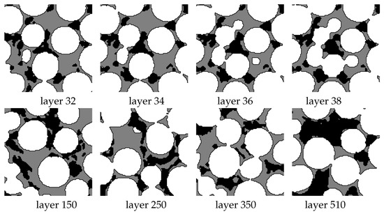
Figure 2.
Pore-scale data with obstructions present with data from [6] on biofilm. All images are at resolution . Region is in black, in white, and in gray. Shown are horizontal slices of column data for different layers, layer 34, which is identical to (a) in Figure 1. The original porosity for this layer is decreased to with the corresponding relative volume of obstructions . The obstructions are pore-coating at lower as well as when vertical slices are considered.
These challenges motivate the alternative methods we explore in this paper.
Aim of this paper. Our goal is to propose a practical method to approximate the connection between and K, specific to a particular process which obstructs the pore space, while allowing and taking advantage of the inherent randomness of the problem. We focus on the case when the pore space is being obstructed by a new solid phase, leading to the change in flow paths, clogging of the pores and the decrease in and K. In particular, we consider microbial growth leading to the plugging of porous media as well as the process of crystal formation and phase transitions. These two processes create obstructions of the pore-coating and pore-filling type. Other important scenarios not explored in this paper include the dissolution of the rock grains, which leads to the increase in and , or to the rearrangement and local changes in and K due to mechanical deformation.
Our approach to connect to K includes three steps: (1) generation of independent realizations of obstructions in , followed by (2) flow and transport simulations at pore-scale, and (3) upscaling. Step (1), the generation of new solid obstacles appearing in some original unobstructed , can be done in several ways, which exploit computations and randomness in many different ways. Steps (2–3) to calculate and K for the given or its REV subset are fairly standard, as we explain in Section 2. In all cases, the variable responsible for the solid appearance is correlated with .
We consider three methods (1A–1B–1C) for step (1), and we follow with the same workflow for (2–3) for each.
First, we consider (1A) Direct Numerical Simulations (DNS) of the actual physical process underlying the changing for the microbial growth application and pore-coating obstructions. Each instance of the (Monte Carlo ensemble of) DNS requires an initial condition, which is assumed to be random, and leads to an instance of of . After steps (2–3), each gives and , which we collect in an experimental probability distribution for built from . Unfortunately, DNS are extremely complex and depend on a multitude of parameters which may or may not be possible to calibrate. Rephrasing, DNS give very specific answers to what may be a very non-specific question.
Because of this complexity, we propose two new computational evolution algorithms (1B, 1C) which are surrogates of DNS of lesser complexity and are designed to generate plausible independent realizations for a given fixed . These eventually give an experimental probability distribution for from the collection . The two new models produce results similar to the known experimental and imaging results as well as to DNS. Both models share a design: they generate by finding stationary states of an evolution towards local minima of a certain non-convex design functional, which determines the quality of the fit of to a particular design of interest. We find these local minima in one of two ways, which we call (1B) Constrained Localized Phase Separattion (CLPS) and (1C) LP.
(1B) is the Constrained Localized Phase Separation (CLPS), which seeks stationary solutions to a partial differential equation, a continuum gradient flow model, and is our proposed modification of the well-known phase separation Allen–Cahn model. In turn, (1C) is the (lattice at pore-scale (LP) model, a discrete model which finds the states of a Metropolis algorithm adapted to pore-scale. Both CLPS and LP are initiated with a random initial state and calibrated to the desired qualitative behavior, consistent with the images from the literature. When run multiple times, we find as many independent realizations I as desired.
Broader context. First, this work is an alternative to traditional multiscale models which use a fixed pore-scale geometry [7,8,16,20,23] to calculate the corresponding Darcy properties. Instead, we consider ensembles of geometries which change to reactive transport. Our entire process is equivalent to creating off-line reduced models of certain quantities of interest, and is a computationally attractive alternative to DNS, which itself is an in silico alternative to imaging and experiments.
This work therefore fits in the area of reduced models [24] as well as in the emerging area of multifidelity approaches [25]. These create a hierarchy of models which approximate the same output but with a different fidelity or modeling accuracy. Our paper addresses the specific challenges of multifidelity and reduced models in the area of pore-scale modeling and upscaling. Specifically, the outputs of our models are pore geometries produced by the DNS, CLPS, and LP models (high-, intermediate-, and low-fidelity models, respectively). While we do not define any metric to compare these outputs, i.e., the geometries, directly, we do so indirectly after upscaling when we compare the Darcy-scale quantities.
We find that, overall, the reduced models CLPS and LP produce geometries which are visually similar to those generated by DNS. Furthermore, the Darcy scale quantities calculated by upscaling are naturally also very similar between DNS and the reduced models. The LP method is very fast but is also somewhat sensitive to the grid resolution and may produce rugged structures at a low obstruction volume. The CLPS method is a bit harder to calibrate and more computationally involved but produces results closer to the DNS. All methods produce upscaled quantities which agree well with those known from the literature for pore coating (mild decrease in K) and pore filling scenarios (dramatic decrease in K).
For upscaling, we draw upon our prior work in collaboration with physical scientists [6,18]. In particular, we set up flow experiments with flow rates in the linear laminar regime, as established in [1,7], and we compare the resulting permeability reduction to those cited in [26,27].
We see possibilities to expand on this work in the future and, in particular, the need to define precise metrics of comparison between the geometries with some form of shape analysis, as well as to connect these results to the data from imaging. Finally, the calibration of the LP and CLPS models was done heuristically, but we envision that it could be guided by some of the emerging data science approaches.
Overview. The outline of this paper is as follows. In Section 2, we define the notation and motivate our interest in the obstructions of two particular types, called “pore filling” and “pore coating”. These are important in two separate fields, respectively, hydrate crystal and biofilm modeling. We also explain how to post-process our geometry with steps (2) and (3). In Section 3, we present our (1A) DNS model for pore-coating associated with microbial growth. In Section 4, we present the (1B) CLPS model, and in Section 5, we present (1C) the LP model. In Section 6, we present our results and discuss the complexity of the three methods and sensitivity to the parameters. We close with a Summary and an Appendix with auxiliary tools and details.
2. Motivation and Notation on Modeling Obstructions
In this section, we explain the specifics of porous media and define the notation. A physical process taking place in porous media can be modeled at Darcy scale and at pore scale. The Darcy-scale models rely primarily on empirical data obtained for cores extracted from soil and rock, and the pore-scale models rely primarily on imaging and micro-fluidics experiments. In this paper, we focus on fluid flow of water, with viscosity , and reactive transport with phase transitions.
Numerical simulation of flow and transport aids in the understanding of and helps to optimize human-engineered systems involving porous media, including oil and gas recovery, remediation of contaminated aquifers, and biomedical applications in human body. Traditional practical models of porous media such as aquifers or hydrocarbon reservoirs [1,28] are posed at the Darcy scale.
In principle, one can also simulate various processes at the pore-scale, which delivers more precision. However, the complexity of the transient flow and transport computations is enormous; see [6] for various simulations of flow alone in realistic 3D pore geometries of synthetic porous media and sandstone. See also [29] for the repository of 3d pore-scale images.
In this paper, we propose reduced models for the multiscale connection between the pore scale and Darcy scale. We consider a porous domain , an open-bounded set with . The position variable has d components, and so do vector valued variables such as velocity u. We denote by , with , where is the usual Euclidean distance between the points .
2.1. Porous Media: Pore Scale and Darcy Scale
Porous media are materials in which the space available to fluid flow and transport is mixed up with solid impermeable particles (rock) aggregated in .
The pore scale is the scale of to at which one recognizes the pore walls, e.g., the interface between the pore (void) space and the solid matrix. We have that
where .
The Darcy scale is the scale of or above, at which the study of flow and other properties does not recognize and but rather relies on average properties found experimentally in a laboratory using core samples. In particular, porosity (volume fraction) is of interest, and permeability K, the coefficient of proportionality in Darcy flow between volumetric flow and pressure gradient. The coefficients and K lump the geometrical information about and . In practice, one uses the probability distributions around some known mean; here, refers to the uncertainty.
Imaging. In this paper, we work with geometries of and found from imaging. See Figure 3 and Figure 4 for illustration of a slice D from x-ray ct or (micro) -CT tomography. In such an image, D is covered by a union of cells , also called voxels. For simplicity, we will assume henceforth that every voxel is a cube of volume , with the side length h fixed by the -CT equipment used. For simplicity, we also assume that every D is rectangular. In particular, as in Figure 3 , , with denoting. Notation when or is analogous.

Figure 3.
Many-pore geometry with obstructions. D is a vertical slice from -CT column, with voxels. With voxel size equal , we have , , and . Rock is in black, fluid space is in blue, and obstructions are yellow. Left: unobstructed pore geometry with and . Middle, right, and far right: pore-filling (middle) and pore-coating (right) obstructions and generated by lattice at pore scale, LP algorithm. Far right: pore-coating obstructions simulated with direct numerical simulation (DNS) method for biofilm nutrient denoted later as BN.

Figure 4.
Single pore geometry with voxels. Left: unobstructed pore with , and . Middle: pore-filling obstructions (hydrate-like). Right: pore-coating obstructions (biofilm-like).
Obstructions and their volume. In many important applications, the pore-scale geometry changes due to various bio-chemical processes, e.g., due to microbial growth, or crystal precipitation. The flow domain itself is thus made of the void space , which is filled with ambient fluid, and of the obstructions in , which are impermeable or partially permeable to the flow and transport. We have that
where . In this paper, we consider solid obstructions which form due to the particular bio-geochemical reactions such as crystal precipitation, or biofilm growth. We motivate and describe these below, and illustrate these first in Figure 3.
To quantify the presence of the solid obstructions, we define
The reference porosity is the initial value of porosity before obstructions form, the current porosity is the volume ratio of space available to fluid, excluding obstructions to the entire porous domain, and is the obstruction volume ratio relative to the original volume of .
2.2. Motivation and Models for Pore Coating and Pore Filling Obstructions
Our main interest is to consider pore-coating and pore-filling obstructions. These two completely opposite characteristics are motivated by our long-term modeling projects with an impact on environmental and energy resource studies involving computational models of microbial growth [6,30] and methane hydrate modeling [31,32,33] in porous media.
2.2.1. Pore Coating Obstructions: Biofilm
Scientists and engineers use microbes to alter the flow paths in porous media in various applications. The understanding and quantitative modeling of microbial growth in porous media is important, e.g., in selective plugging for the needs of enhanced oil and gas recovery, as well as in carbon sequestration [34,35,36,37]. The microbial growth is promoted by providing nutrients. The microorganisms form a special extracellular polymer substance (EPS) of high density, which is impermeable or almost impermeable to the external flow, and which typically clings to the pore walls. EPS protects the microbes but clogs the pore void space. In particular, a reduction in permeability is significant; see, e.g., [6,38,39,40].
The experiments and DNS show that the biofilm growth and the Darcy-scale properties depend on various conditions at which the growth occurs, e.g., on flow rate. However, imaging biofilm is intrusive and harmful; thus, it is close to impossible to predict for the growth in a variety of different conditions. We present a DNS model of biofilm-nutrient (BN) dynamics at pore scale in Section 3.
2.2.2. Pore Filling Obstructions: Hydrate Crystals
Methane hydrate is a naturally occurring and highly concentrated form of methane: a crystal lattice comprised of frozen water cages trapping gas molecules. It holds significant quantities of carbon in the global system but forms in areas of low temperature and high pressure and is abundant in permafrost and marine sediments. It is important in energy and environmental studies as an energy source and potential climate accelerant, and some modeling and experiments have been forthcoming [27,31,33,41,42,43]. In particular, it is known that, at low , the hydrate grows in the pore centers and causes significant changes to the permeability and sediment strength; see, e.g., the experiments in [44].
However, observations and experiments on the impact of hydrate on permeability are challenging due to the requirements of low temperature and high pressure needed for their stability [41,45,46,47]. Thus, it is difficult or very expensive to obtain experimentally or to image for hydrates.
In turn, DNS for phase field models for hydrate are very complex and dependent on a multitude of parameters, as shown in [48,49]. We have forthcoming work on the pore-scale models of pore-filling crystal formation, but providing DNS here is out of scope.
2.3. Obtaining Darcy Permeability K with Computations
K depends on the connectivity within in a nontrivial way. Some experimental algebraic correlations for assume a particular simple form of . For example, the Carman–Kozeny relationship assumes that is a bundle of capillaries and postulates , where ; see [1,28].
For more general , the workflow to obtain from fluid flow simulations in is called upscaling or numerical homogenization. For laminar flow, the permeability K is found by (2) finding the solutions to a viscous flow model at the pore-scale, and (3) upscaling .
One additional consideration in pore-scale simulations is whether D used in Algorithm [Pore2K] (Algorithm 1) is a Representative Elementary Volume (REV) large enough for it to make sense to consider its Darcy scale properties as representative. This important issue was considered in, e.g., [20]. For example, consider the illustration in Figure 5, in which we show a realistic image from -CT as well as an idealized single-pore geometry. With studies in [50], we find that the one-pore domain is sufficient for the study of quantities of interest related to the flow, but may not be adequate for transport-related quantities.
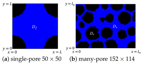
Figure 5.
Notation for pore-scale domains used in simulations. Domain is blue, is black. Left: domain D for single-pore experiments. Right: domain D for many-pore experiments, an imaged representative elementary volume (REV) from [6]. The single-pore domain on the left is an idealized subset of the many-pore domain on the right.
| Algorithm 1. Algorithm [Pore2K] for obtaining from |
| Given we calculate from (3). Next, we solve the velocity and pressure satisfying the Stokes system in with the no-slip boundary condition on the pore walls, inflow condition on the portion of , and a natural outflow condition on the outflow part |
| To approximate the solutions to (4), we use an MAC scheme extended to Brinkman flow, which we implemented in MATLAB as described in [30], or the computational environment HybGe-Flow3D [16,51]. |
| The approximations to are averaged over D to U and P, respectively, and fit to the Darcy model
|
| In particular, we find U by averaging over |
| From these, the permeability tensor K is calculated. See, e.g., [7,19,20] for a detailed description of this workflow, including setting up multiple flow scenarios to provide sufficient information to calculate the full tensor K. In this paper, we report only on one scalar value of K, the component corresponding to the flow from left to right. |
Example 1.


We simulate flow with (4) in a “many–pore” geometry . We consider the case with and without obstructions, and consider of both pore-filling and pore-coating type. We set the flow to go from left to right, with the average of through on the left, and on the right; see Figure 6. The flow rate is in the linear laminar regime and is similar to that used in [6]. The parameters used are in Table 1.

Figure 6.
Illustration of flow in Example 1 with , (a) no obstructions and , (b) hydrate-like pore-filling obstructions, (c) biofilm-like pore-coating obstructions. In (b–c) . Shown are normalized velocity magnitude as well as the streamlines. We follow up with calculation of permeabilities and obtain (a) , (b) , and (c) .

Table 1.
Parameters for the flow example in Example 1.
2.4. Flow: From Pore-Scale to Darcy Scale with Obstruction Formation
When obstructions appear in , they clog the pore space and significantly alter the flow and transport paths in , and the quantities and K decrease from and , respectively, see illustration in Example 1 and Figure 6.
To quantify this change, one can run physical flow experiments or imaging in parallel to the obstruction formation to obtain and . However, to our knowledge, such a set-up is extremely challenging, since it requires stopping the reactions somehow at fixed time intervals to run the flow experiment. In consequence, it involves large uncertainty. Therefore the sampling is frequently limited to only few time steps: the beginning and the end of experiment; see, e.g., [6,41] for the study of for hydrate crystal formation and of biofilm clogging, respectively. However, such imaging efforts in real time are very costly and time consuming and pose additional technical challenges, including how to stop the process for the purposes of imaging. For the applications of interest, including both the biofilm and hydrate applications, as detailed in Section 2.2, it is close to impossible to image at a fine resolution of t.
Instead, an unobtrusive way to understand how the pore-scale geometry is changing with time is to use Direct Numerical Simulations (DNS) of the underlying bio-chemical process at the pore-scale; see, e.g., the models in [52] or [6,30]. DNS are very appealing because they seem to closely represent the physical reality. However, they involve a multitude parameters with large uncertainty, including the initial conditions. Unfortunately, their complexity is also enormous: they require 3D simulations with O (10 M) cells and many time-steps, and thus cannot be used easily in multiscale scenarios involving simulations of complex coupled systems.
The general strategy to overcome this complexity is to consider reduced or surrogate models [24]; see also our pore-scale-related work in [16]. Reduced models exploit data collected or produced off-line in a library of simulation results to provide answers to queries on some desired quantities of interest. For the case considered in this paper, such a library can provide answers to a query on, say, sampling K from for a given and a given type of process, e.g., microbial growth or hydrate growth. More generally, answers can be provided for pore-coating or pore filling scenarios, with an associated measure of uncertainty. In the current era of data science, these models or queries can be replaced by neural networks.
The methods proposed in this paper are the third way (iii) to create experimental distributions of . In an abstract setting, they deliver surrogate or reduced models of the true DNS–derived distributions, and they do so very efficiently. While our simulations are not based on first principles, the geometries we generate are similar to those found by -CT imaging.
2.5. Transport from Pore-Scale to Darcy Scale
The Darcy coefficients and K are important for modeling the flow. For transport, other important quantities of interest at Darcy scale are the tortuosity and breakthrough curves relevant for transport models.
First, we recall the transport model at pore-scale. Once the velocity is known from (4), we can simulate the advective transport, the first-order PDE
The inlet value is constant, and in our experiments, we set .
To understand the impact of geometry of pore-scale on the transport at the Darcy scale, we can upscale the transport solution c by averaging over D to obtain
but a lot of information is lost in this step. As is widely known, it is useful in this context to consider the notion of tortuosity discussed in detail, see, e.g., [1,53] for various definitions and uses. In particular, the tortuosity helps to distinguish channel-like pores from those of more intricate shapes. For the left-to-right flow considered here, we calculate hydraulic tortuosity , where L is the “straight-line” distance in D from left to right, and is the effective path length taken by the fluid through . The path length for each streamline is easy to find, and is found by averaging over all streamlines. In addition, we recall the breakthrough curves which assess the average time it takes to travel through D
To compare the breakthrough curves, we also define
This -breakthrough time is the time when the pore is at percent of the total possible outflux.
The tortuosity and breakthrough curves provide information on the transport that is partly lost in upscaling. In particular, tortuosity is used to identify dispersion in the porous medium.
To find and the breakthrough curves, we apply Lagrangian and Eulerian methods, respectively. In the Eulerian frame, we approximate the solutions to (7a), and calculate with an explicit upwind Finite Volume scheme known as Donor in Cell [54]. The method is stable if the time step satisfies the Courant–Friedrichs–Lewy (CFL) condition. In the Lagrangian frame, we first find streamlines for the flow by explicit time-stepping of starting from , and using the approximation to u interpolated on each cell from the solution to (4). Next, we propagate the constant value of c along the streamlines from to . In the Eulerian frame, we approximate by summing over the cells adjacent to . In the Lagrangian frame, we track the position of the front of each streamline s at time , and approximate by summing the number of streamlines that have reached the outlet before .
Summary. We have identified the important quantities that will be used to study average properties of porous media at Darcy scale from the knowledge of the pore-scale geometry of the void domain . In the sections below, we present methods (1A–1B–1C), respectively, which generate the realizations of . We denote the upscaled quantities with subscript i. In addition to porosities and permeabilities , we consider and .
3. DNS for Single-Pore Geometry with Obstacles of the Pore-Coating Type
In this section, we generate multiple realizations of obstructions using the DNS of the process of biomass-nutrient (BN) dynamics. This process creates pore-coating obstructions, as noted in [6]. We consider a fixed and a fixed . Our DNS produces the domains and, equivalently, their complements in .
The model we use was first proposed in [6], recently refined in [30], and is further modified to reinforce the pore coating behavior.
3.1. Biomass-Nutrient Model
Let represent biomass and nutrient concentrations, respectively, chosen in convenient non-dimensional units. Let denote the maximum possible biomass density, and the threshold, such that the region represents the mature biofilm phase, which contains microbes as well as the biomass-produced extracellular polymer substance (EPS). This substance is beneficial to the microbes as it provides a safe environment for growth. For the purposes of this paper, we therefore consider that obstructions are the same as the quite dense phase
To model biomass growth and formation, we consider the model simplified from that in [6,30]
Here, the nearly singular diffusivity is parametrized by , motility and , and given by
The Lagrange multiplier enforces the constraint . (Here, denotes the subgradient of the indicator function of a set S). A numerical solution of (12) is challenging due to the nearly singular behavior of , and the presence of , which makes (12) a nonlinear parabolic variational inequality.
We use the linear diffusivity model for N
where the nutrient diffusivity in , which is close to the molecular diffusivity of water, and in .
We also have the biomass growth, and the nutrient consumption rates are given as
with the utilization rate in , the specific substrate uptake rate , and the Monod half . In this paper, we focus on the nutrient rich case and assume that is large enough.
The role of in (12j) is to “promote” the pore-coating behavior of biofilm. This is a well known feature of microbial growth: the microbes stay close to the wall, which provides protection to the community from detachment and other mechanical deformation due to large flow rates; they achieve this by excreting an adhesive substance which supports this mechanism. However, this pore-coating behavior is difficult to calibrate quantitatively, and we choose to do this by heuristically decreasing the reaction rates from according to the following model, depending on a parameter A, as in (12j), where is the solution to the Poisson equation with homogeneous Dirichlet boundary conditions on and Neumann boundary conditions on . For illustration, we provide the plot of in Figure 7. With , , and the rate . However, with , we see that as the distance from the wall increases, .

Figure 7.
Contours of the attraction coefficient defined by (12j) in single–pore geometry and many-pore geometry.
Finally, we close the system with initial conditions (12e) and (12f), and we choose to include only the voxels immediately adjacent to the wall of , so that with a given . This choice is consistent with the usual assumption that the porous domain is inoculated with microbes which settle down next to the wall .
3.2. Results of the DNS Model for Dynamics
We start with a single-pore geometry , in which we let evolve from initial state .
We use parameters listed in Table 2 and perform Monte Carlo Simulations with a collection of I realizations of , which lead to the biofilm evolution and formation of obstructions . A few examples are shown in Figure 8 (top) for and .

Table 2.
Parameters for the DNS model and simulations of described in Section 3.1. Simulations cases (a,b,c,d) are presented.
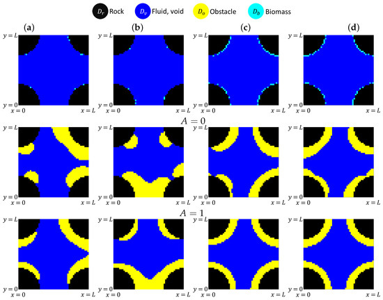
Figure 8.
Generation of with DNS for single-pore geometry , with simulation parameters for cases (a–d) are given in Table 2. Top row: randomly chosen regions used for initialization in (12e) for each case (a–d), with small relative volume in (a,b) and larger volume in (c,d). Middle and bottom rows: regions obtained with BN model at the time when the corresponding obstruction volume ; each region was obtained by simulation with initial conditions shown in the top row, respectively. Smaller and corresponds to less pronounced coating behavior.
The biomass in each case evolves first, and the biofilm phase becomes mature and impermeable when . Next, this phase continues growing by interface creating new obstructions , whose volume increases over time. The growth pattern depends on the initial state. Figure 8 (middle) and (bottom) show biofilm distribution evolved from the initial states Figure 8 (top) with and , respectively.
With and small , we see that the biofilm tends to grow spherically without strictly adhering to the walls. However, when we increase to cover evenly, the biofilm sticks together but grows gradually away from walls.
On the other hand, with , the growth away from the walls is suppressed to promote growth near the walls. We see a dramatic difference as compared to the case when .
4. Reduced CLPS Model: Constrained Localized Phase Separation
In this section, we describe our phase separation model. We work with a function called the phase or order parameter, defined in the pore-scale domain and evolving in time t. The function is a solution of a certain partial differential equations called phase separation model. We approximate with a finite difference scheme on the grid covering ; see Appendix. We post-process the numerical solution to obtain .
The phase separation models in the literature include the Allen–Cahn (AC) and the Cahn–Hilliard (CH) Equation [56], often studied together as gradient flows of the functional
The parameter has the physical meaning of the interface width, which arises due the competition between the diffusion and coarsening; it also affects the time scale of the evolution; see, e.g., [56,57]. The potential energy density part of (13) is typically a non-convex function with two stable minima and , and an unstable local maximum between these. One common choice is , which corresponds to the solid phase, and , which corresponds to the liquid phase, with the energy density given by the “double well” function . Non-polynomial functions, such as in Ginzburg–Landau models, are also possible [56].
The gradient flow
for in (13) is the Allen–Cahn (AC) equation which describes the evolution of towards one of many stationary solutions ; these are the local minima of . The dynamics of the resulting semilinear parabolic PDE are well known: the stationary solutions feature patterns with aggregation in the regions
with some diffuse interface region separating and of width proportional to , due to the competition of diffusive and reaction terms associated with and , respectively. Various rigorous analyses are available; see, e.g., [58]. With bounded initial data in , the solutions evolve towards one the (multiple) equilibria for .
In this paper, we exploit the ability of AC model to produce patterns as the main design idea, but we modify the model to fit the interactions with the boundary of D, as described next.
4.1. Volume Constrained Phase Separation CLPS Model
We exploit the non-convexity of and the non-uniqueness of the stationary solutions to the AC model as the main design idea. We aim to generate patterns of region with obstructions with a certain given prescribed volume , and we aim towards . We choose to denote cells with obstructions and (no obstructions). With these, we obtain that
We pose the AC model, the gradient flow of (14) in
where, for , we use the double-well potential density and its derivative
The solutions to (17) aggregate in the regions
Typically, these regions , are non-empty and they stabilize as , and as the values of separate on the path to stationary solutions. However, the volume of obstructions is not preserved. This can be seen by integrating (17) over and applying Neumann boundary conditions.
As part of our algorithm, we aim to maintain
We impose this equation as a constraint, and follow the general strategy outlined in [59]. We augment by the term with a Lagrange multiplier . The resulting evolution model for reads
4.2. Controlling the Location of Obstructions in CPS with Localization in CLPS
Consider now a given pore-scale domain D, with and known, as shown in Figure 4, and a simulation of the CPS model (20) in . Starting with some initial condition, the model will produce aggregated patterns of obstructions indicated in (18), but with the aggregates in somewhat randomly located in . In particular, these aggregated domains may be close or far from , and therefore will not adhere to a pattern with qualitative properties consistent with the “pore-coating” or “pore-filling” behavior illustrated in Figure 4.
To rectify this, we modify the CPS model to promote the desired qualitative properties of . In particular, we want to control the shape of and its distance to , as we promote the formation of obstruction with the “pore-coating” or the “pore-filling” behavior. In the pore–coating behavior, the obstructions aggregate adjacent to the solid matrix so that the distance is small. In the pore-filling behavior, they aggregate away from the solid matrix and is as large as possible. In other words, in the pore-filling behavior, , is “repelled” from , and in the pore-coating behavior it is “attracted” to .
Such behavior can be realized by an application of some form of physically motivated “taxis” towards or away from . In particular, one could set up the taxis with the gradient of an electrostatic or van der Waals potential to model the actual physical attractive or repulsive forces towards or away from . In particular, such taxis can involve electrochemical interactions such as those included in the work on Poisson–Nernst–Planck models as in [61,62,63]. These complex models require a multitude of physical parameters that might be difficult to measure and require additional computations.
To avoid this additional complexity, we choose instead a simpler heuristic approach, which we call the Constrained Local Phase Separation (CLPS). The model modifies (20) and reads
and is a modification of (20), which we amend with a spatially varying source function , with parameter , allowing additional control on the localization, and define
See Figure 9 for illustration.
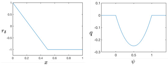
Figure 9.
Components and of the auxiliary function from (21e) with and . As , and . In contrast, away from , we have and .
Properties of the Solution to CLPS
The dynamics of (21) are competition of coarsening due to , diffusive action of , and the localization function , which is only active when . The solution to (21) maintains its total volume due to the Lagrange multiplier construction and Neumann boundary conditions. Additionally, the interplay of and is most interesting.
When , we work with the dynamical system to see that at each x, the solutions tend towards one of the two stable equilibria and , but may also remain at the unstable local maximum of . The action of as in (17) provides spatial variability and allows the patterns of the sets and to emerge and coalesce.
When , the dynamics of individual components of (21) are nontrivial. In particular, even the stationary problem in 1d alone, with homogeneous Neumann conditions, has exactly two solutions , and .
More generally, consider and the ODE , with a stable equilibrium , and an unstable one at . Adding to the right hand side, as in the ODE , does not change the qualitative nature of this evolution towards the stable equilibrium . In contrast, if and is large enough, the stable equilibrium is “promoted” in spite of the competition between and . The presence of leads to the formation of patterns.
Finally, consider the term with . Close to , the effect of is to “encourage” . Away from , we see that ; thus, this choice leads to the formation of patterns with “pore-coating” behavior.
On the other hand, if we obtain “pore-filling behavior”. If is large, then, close to , we encourage , and away from the boundary towards . In other words, we obtain the pore-filling behavior.
4.3. CLPS Model to Generate Multiple Realizations of Obstructions in Pore-Scale Domain
Consider now simulations of (21) in a domain which is a realistic 2D slice of a pore-scale domain from -CT experiments from [6,7,8], with rock domain , shown in Figure 3. For this domain, we have a discretization parameter relative to the domain size ; we provide an outline of the numerical scheme in Appendix A.
We must choose the desired volume of obstructions , and the parameters , and , which control the qualitative nature of the domain with obstructions. We recall that controls the width of the interface close to . With , we promote pore coating, and with , we promote pore filling. The choice of and is guided by heuristics and intuition, so that has the desired characteristics when assessed visually. In the future, we plan to guide the choice of parameters by a systematic approach guided by data science. Typically, we choose and . See Table 3 for a summary of all the parameters.

Table 3.
Parameters for CLPS model from Section 4.3 in single-pore and many-pore geometry. The model uses nondimensional rather than physical units.
The Algorithm CLPS (Algorithm 2) has (A) a pre-processing stage in which we choose parameters, (B) simulation of , and (C) post-processing step, in which we use to determine .
| Algorithm 2. Algorithm CLPS [A-B-C]: for a given and , generate a possible |
| CLPS [A]. Set parameters . |
| Pore–coating: set . |
| Pore–filling: set . |
| CLPS [B]. Choose some random and run the transient simulation of (21) until , when the system seems to reach a stationary solution. In practice, we run the simulations until reaching large , such that for , the solution does not change significantly. |
| CLPS [C]. Post-process and set and based on the value of the cell-centered approximation to found in (B) on the voxel grid covering . |
| Now, as seen in (18), the stationary solution is close to the characteristic function of . Thus, we assign the cell to when , and to whenever . However, when , we must make a choice so as to honor (19) with the fixed . We can do so by assigning to if , and to , otherwise, where is some threshold value chosen depending on : this strategy supports the interpretation that represents the amount of obstruction material contained in cell . Alternatively, we assign a certain number of cells to with the highest value of selected randomly; this strategy is easier to implement than the former. |
We can repeat the algorithm CLPS as many times as desired. Since we aim to obtain a large number of realizations, we consider a collection of “white noise” random initial conditions which satisfy (19), and which are generated by a uniform random generator on the voxel grid for . We seek a collection of stationary solutions , where , and the corresponding post-processed obstruction region .
Example 2.
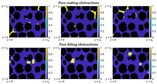
Consider the parameters in Table 3. and the many-pore geometry shown in Figure 3, and set . In Figure 10, we present two of the many stationary solutions obtained for each case, where we choose and apply algorithm CLPS. We plot the contours of the stationary solutions , which satisfy . These are later used in flow simulations with the post-processed results discussed in Section 6.

Figure 10.
Contours of selected stationary solutions , to (21) found with CLPS model from Section 4.3. The solutions are post-processed to give as described in Section 4.
5. The LP Method from Statistical Mechanics to Generate Obstructions
In this section, we present a method called the LP method to generate geometries with obstructions. Unlike CLPS (21), which is a PDE for the minimizer(s) of the functional in (13) under constraints, the LP method does not use any differential equation, and is motivated by statistical mechanics models of phase transitions from the class of dynamic discrete lattice models from [64,65].
We recall the Markov Chain Monte Carlo (MCMC) method, and, in particular, the Metropolis algorithm [66,67,68], in a setting similar to the Ising model, as in [67]. The Ising model is widely known as a tool for generating arrangements of spins on a lattice, with applications in the study of phase transitions. In this paper, we apply it to the pore-scale geometries represented on a lattice, hence the name LP. We are motivated by the work in [69,70], which in [71], we adapted to multi-component adsorption. We modify the setting from [71] to the present case of pore-coating and pore-filling geometries from -CT. We explain the case of lattice, but an extension to is immediate.
We start with a given digitized rock image D from -CT, and a given . The practical objective is to assign each voxel of the voxel grid covering to either or . This is equivalent to setting an indicator variable to one of three values indicating the void region, rock, and obstructions, as follows
Now, each can be considered as a node of a lattice, and we collect these in the vector . For a collection of realizations, we denote the i’th realization by , with the corresponding , . We start from some initial configuration , and we seek its stationary state, , a local minimum of a certain non-convex Hamiltonian functional , which determines the quality of the fit to our particular design of interest. We find these local minima using the Metropolis algorithm.
After the ensembles of geometries are found, we post-process each one to get and to calculate the porosity , permeability and tortuosity .
5.1. LP Model for Minimization of a Hamiltonian Functional Defined on a Lattice
Next, we define the Hamiltonian energy functional , which assigns some energy to each X. This Hamiltonian depends on various parameters which eventually lead to different cell aggregation patterns. In particular, we consider the aggregation patterns of the pore-coating or pore-filling character.
5.1.1. Hamiltonian for Generation of Obstructions
In the design of , we include weights for the interaction at each type of interface between the lattice nodes in , and . The weights allow control over the qualitative character of the configuration of obstructions, such as in the pore-filling or pore-coating patterns.
Consider the node and let denote its immediate neighbors. Let the next nearest neighbors be defined as
We use periodic boundary conditions; thus, any of the nodes in and are well defined.
Next, we set some weights , , and and associate these with the rock–obstruction, rock–void, and void–obstruction interfaces, respectively. Now, we define
We also let be the weight of the next-nearest neighbor interactions, and define the Hamiltonian
As usual, we use the Boltzmann distribution where Z is the normalizing factor, is the Boltzmann constant, and is the inverse temperature. We follow the literature closely [64,65,67,68].
5.1.2. Metropolis Algorithm for Pore-Coating and Pore-Filling Obstruction Patterns
The Metropolis algorithm for minimization of starts from some random initial configuration to produce the chain, which evolves towards one of the local minima of . The algorithm is inherently stochastic. In each step, the method rearranges the assignment of the cells to to find the configurations which are more likely, i.e., have a lower value of energy represented by the Hamiltonian (Algorithm 3). The process is similar to fixing the net magnetic spin in the Ising model and flipping randomly chosen spins so as to find a configuration corresponding to finding one of the local minima of .
| Algorithm 3. Algorithm LP [A-B-C] |
| LP [A]. Generate the initial state randomly for the given . |
| Choose parameters and W, ; see Table 4. |
LP [B]. and follow with iteration for updating for as follows. Let .
|
| Continue the Markov chain until satisfied that the so-called “burn-in” process is completed. Stop the iteration at some . |
| LP [C]. Postprocess the final state which corresponds to one realization of pore geometry with an obstruction. Specifically, the nodes corresponding to identify the voxels in . |
Notice that a different corresponds to a different , i.e., a different realization of .
5.2. Results of LP Model for Single-Pore Geometry
We now illustrate the algorithm for as shown in Figure 4. The -CT data provide the resolution with . We also choose , . To obtain pore-filling and pore-coating obstructions, we set set the weights, as in Table 4, which avoid or promote the clinging to rock matrix and tend towards clumping.
In Figure 11 we show the progression of the LP model for generating the obstructions for pore-filling. We see that the obstruction cells quickly aggregate. However, it takes many steps for the process to stabilize with a single clump.
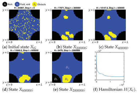
Figure 11.
States of the LP process for the formation of an obstruction with weights given in Table 4. Rock matrix is black and void space is blue, while the obstructions in are yellow.
We next consider the generation of obstructions that favor adjacency to the rock matrix. The chosen weights also discourage the formation of fingers of obstruction. In Figure 12, we show the progress of the LP model. We can see that the obstruction cells form a thin layer along the rock matrix. The burn-in time for this process is much shorter than in our previous example.
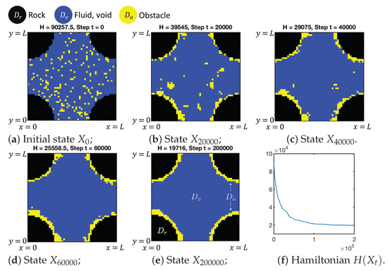
Figure 12.
States of the LP model process for the formation of an obstruction from Section 5.2. Rock matrix , is black, void space is blue and the obstruction is yellow. .
6. Results and Comparison of DNS and Reduced Models
In this section, we compare the three methods of generating domains with obstructions. For the pore-coating scenario, we compare a method of generating obstructions from (1A) DNS (BN) from Section 3, (1B) CLPS from Section 4 and (1C) LP from Section 5. For the pore-filling scenario, we only consider (1B) and (1C).
The workflow in our experiments is as follows. We start with a porous domain with some known , i.e., with some known initial porosity . This domain may be either a many-pore model, such as from -CT imaging, as shown in Figure 3, or a smaller idealized single-pore model, such as in Figure 4. We choose the type of obstructions from either biofilm (pore coating) or hydrate (pore filling). The generation of obstructions is followed by simulations of flow and transport in and upscaling to Darcy-scale parameters impacted by the presence of obstructions; these steps are as described in Section 2. Of interest is the relative change in the upscaled quantities from their unobstructed values denoted with subscript “0”, e.g., or , corresponding to .
The first method (1A) produces I independent realizations with DNS for the pore-coating scenario, with the associated . The simulations start with initial conditions localized in randomly chosen grid cells close to , with a fixed initial amount given by parameter , which indicates the total initial biomass amount. We simulate each case up until the timepoint t at which the desired ratio in is obtained, or until clogging, whichever occurs first.
The method (1B) CLPS produces I independent realizations corresponding to a given chosen , with a given , starting from random initial condition . The result of each simulation is a corresponding stationary solution for the evolution, which we post-process to obtain the collection for each . For (1C), the LP model, we set and randomly select the desired number of cells out of the voxels in ; this choice gives the random collection of . We run the evolution until the stationary solutions are found.
The first overall observation is that we find a qualitative agreement between the DNS model BN and the reduced models CLPS and LP both by visual inspection of geometries and through the probability distribution of upscaled properties. There are also some differences, which we discuss in detail. This is of primary importance for our purposes, as we aim towards the creation of reduced models.
We also present additional interesting features for the pore-coating and pore-filling obstructions, which we discuss in detail below. We first focus on flow properties in Section 6.1, and then on transport results in Section 6.2.
6.1. Permeability Distributions in the Idealized ”Single-Pore” Geometry
We consider an idealized single-pore domain D, as in Figure 4. We generate geometries with the DNS model BN, starting with a completely random initial microbial amount situated next to , as shown in Figure 13. We also use this for initial BN with a identical to the regions produced by LP method.

Figure 13.
Realization of used in DNS results: (a) for Figure 16, (b) for Figure 17, (c) for Figure 18, (d) for Figure 19.
Next, we use models LP and CLPS with the parameters shown in Table 3 and Table 4, set with intuition and heuristics. For each type of obstruction and obstruction volume in (25), we generate obstructed geometries, of pore-coating and pore-filling type, for each of the selections
Various snapshots of selected geometries and the corresponding are shown for the single-pore geometry for different methods in Section 3, Section 4 and Section 5. They are generally qualitatively similar to each other within the category of pore-coating or pore-filling, but also feature some differences, revealed by visual inspection. The solutions to BN models depend on how closely we enforce the adhesion of biofilm to the boundary , i.e., on parameter A.
6.1.1. Pore-Coating Biofilm-Like Obstructions
We start by emphasizing the difference between (1A) and (1B–C). We recall from (3) that
Thus, obtained with DNS model (1A) varies (continuously) in time t, but are actually constant for each experiment with (1B) and (1C) when using selected volume fractions from (25). This is shown well in Figure 14 and Figure 15, where we compare the scatter plots of with the results of BN vs. CLPS vs. LP model for the pore-coating scenario.
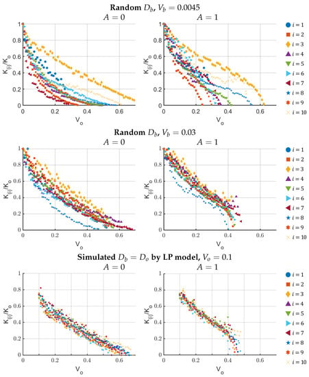
Figure 14.
Dependence of on with the BN model discussed in Section 6.1.1. Results are shown for 10 realizations of geometries, selected out of , generated with and A, as shown.
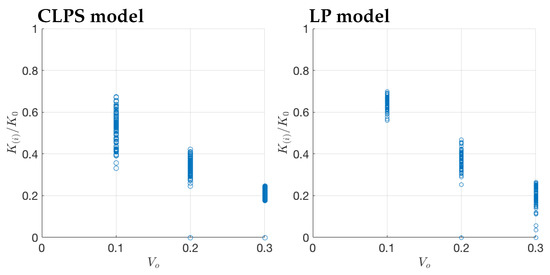
Figure 15.
Dependence of K on when are found with reduced models CLPS and LP discussed in Section 6.1.1.
For BN discussed in Figure 14, the shape of geometries, and thus the relationship between and , depends on how these geometries were created, and, in particular, on the choice of A. We recall snapshots found with BN and shown in Figure 8, and now study the evolution of in Figure 14. We see that decays close to linearly with , with more uniform pore-coating, and is promoted with and large , but we see faster decay of K with or large .
In this context, an important natural question arises. Since all the geometries we create are random, it is not useful to compare them one by one. However, we want to know whether a BN initialized with one of geometries created by CLPS or LP with small will predict evolution towards large which is consistent, on average, with those produced by the reduced models. We confirmed this, and we saw a very close agreement between the distributions given by BN and CLPS and LP, as seen by comparison of plots in Figure 14 (bottom) and Figure 15. This result is desirable but not unexpected, because the geometries corresponding to more tightly prescribed initial conditions tend to evolve in a more predictable way.
Remark 1.
Furthermore, we want to know whether the trends in the decrease in permeabilities predicted by DNS and plotted in Figure 14 are realistic, and how they compare with the realistic data. For this, we recall the model for the dependence of K on based on Carman–Kozeny models for pore-coating and pore-filling scenarios ([27] Figure 4, p. 8), given from algebraic expressions for the pore-coating strategies, and with or for pore-filling. In the range considered here, these formulas predict a mild (linear) decrease in K for pore coating, but a dramatic one (convex) for pore filling, in the shown range of .
Analysing Figure 14 and Figure 15, we see that the case of strong pore coating corresponding to is consistent with the mild linear decrease discussed in Remark 1.
Next, we discuss the histograms and other statistical information on the probability distribution of . We compare the results for BN with and and the different initial biomass domain fraction , CLPS and LP. We consider the distributions shown in Figure 16, Figure 17, Figure 18 and Figure 19 for DNS model BN, and CLPS and LP in Figure 20 and Figure 21, respectively. For each, we present a cartoon of a sample geometry and the statistical information on the permeability distribution for depending on .
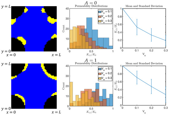
Figure 16.
Results of DNS with and A as shown. Left: one of the realizations for . Middle: histogram of for . Right: mean and standard deviation of for .
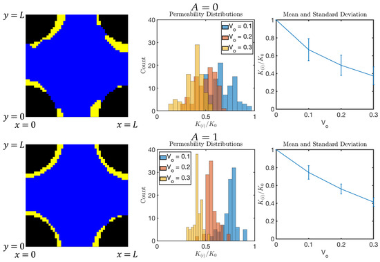
Figure 17.
Results of DNS for and A as shown. Left: one of the realizations for . Middle: histogram of for . Right: mean and standard deviation of for .
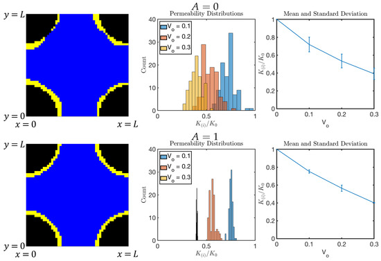
Figure 18.
Results of DNS with and A as shown. Left: one of the realizations for . Middle: histogram of for . Right: mean and standard deviation of for .
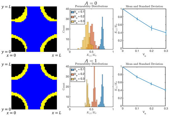
Figure 19.
Results of DNS with A as shown when using from LP model from Section 6.1.1; here . Left: one of the realizations for . Middle and right: histogram of and mean and standard deviation of for , respectively.
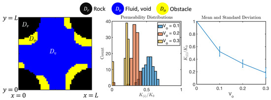
Figure 20.
Results of CLPS model for biofilm-like obstructions from Section 6.1.1. Left: one of the realizations of for . Middle and right show the experimental probability distribution of for three values of .
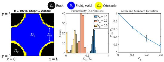
Figure 21.
Results of LP model for biofilm-like obstructions in Section 6.1.1. Left: one of the realizations for . Middle and right show the experimental probability distribution of for three values of .
Studying the sample snapshots of in these figures, we see that the obstructions aggregate in distinct “colonies” for DNS with and for CLPS, but do not cover the entire rock–fluid interface. This feature is dissimilar to the case of DNS with , and to the results of the LP model in Figure 21. It seems that the LP model is tuned to promote adhesion to more strongly than CLPS. The difference between CLPS and LP is similar to the use of and in Figure 16, Figure 17, Figure 18 and Figure 19. Once again, we confirm the same trend for pore coating, consistent with the mild linear decrease discussed in Remark 1.
These observations correlate to the properties of probability distribution for permeability. The distribution for CLPS is less tight than for LP. The histograms of for are symmetric, but less so than for the larger . For the higher values of , we see that, occasionally, the pore space is completely clogged, resulting in for some realizations. The trend in the mean of depending on follows a similar trajectory to that for the LP model, but with a greater variance in . These observations are also similar to those for the DNS model BN and the case and , respectively.
Overall, we infer that pore-coating obstructions, such as in biofilm formation in porous media, may cause somewhat predictable changes in permeability for this range of , but that a larger corresponds to smaller predictability.
6.1.2. Hydrate-Like Obstructions
Next, we tune the CLPS and LP models to produce pore-filling (hydrate-line) obstructions. We use parameters in Table 3 and Table 4.
Results for CLPS are shown in Figure 22. The CLPS model predicts a drop in relative permeability of about one order of magnitude at . For the LP model, the histograms of show a distribution skewed towards the origin, and the change in the mean is sharp, dropping nearly 85% with , but levels off as increases. The standard deviation of is quite large, suggesting a very significant but less predictable impact on the sediment permeability when hydrate crystals form.
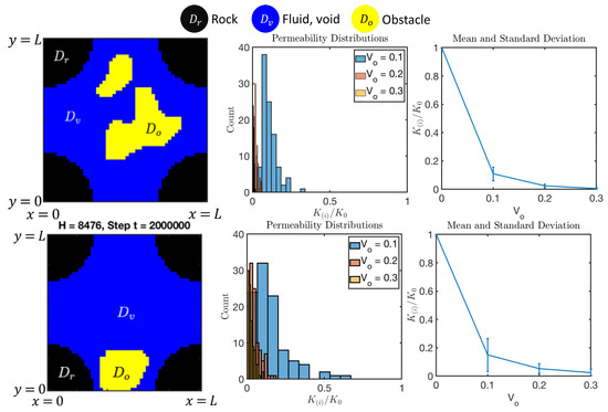
Figure 22.
Results of CLPS (top) and LP (bottom) models for pore-filling in Section 6.1.2. Left: one of the realizations of domain . Middle: histogram of for 3 values of . Right: mean and standard deviation of for three values of .
While the results of CLPS and LP are similar, we note that the CLPS model has a smaller spread with smaller standard deviation as compared to the LP model.
Finally, we see that the trend for pore filling is consistent with the dramatic decrease (sharp drop with a convex graph) discussed in Remark 1.
6.1.3. Disaggregated Obstructions
For additional interest, we here present the results for geometries without any aggregation, of the “free colloid” type. These can be generated by the LP model with parameters, as in Table 4. We show the results in Figure 23 for the distributions corresponding to . We see that he impact on permeability appears much stronger than in the pore-coating or pore-filling case. We acknowledge that this effect may be somewhat overstated, due to our experiments being conducted in 2D and to the coarse grid resolution. Nevertheless, this is a striking result, which speaks for the need to simulate the aggregation and disaggregation of for realistic predictions of permeability.
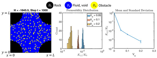
Figure 23.
Results of LP model for disaggregated obstructions from Section 6.1.3. Left: one of the realizations for . Middle and right: relative change in permeability due to colloidal obstructions. Note the log scale used for .
6.2. Flow and Transport Properties in Many-Pore Geometries
In addition to studying the flow in obstructed geometries, it is important to study the transport time at which the outflow reaches some fixed ratio of the inflow of the transported species.
For these studies, we use a large REV with the many-pore geometry from Figure 3. We generate obstructed geometries with CLPS and LP models for each pore-coating and pore-filling obstruction with . For each geometry , we solve for flow and upscale to the permeability . We follow up with transport solutions in the Eulerian frame of reference, and approximate the breakthrough curve as in (9). We study the scatter plots of vs to show that the latter quantity is not correlated to the former; thus, it is important to study both.
Example 3
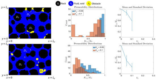
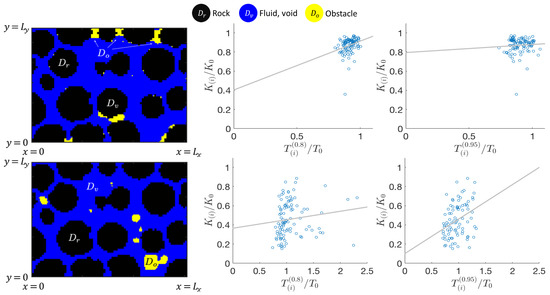
(Many-pore with LP model). We use the parameters from Table 4 for many-pore geometries. We present the permeability results in Figure 24 and transport results for and in Figure 25, with a least squares fit to the data shown as a solid gray line.

Figure 24.
Flow properties with geometries obtained with LP model in Example 3. Top row: pore-coating, and bottom row: pore-filling geometries, Left: many-pore geometry with . Middle: histogram of for two values of . Right: mean and standard deviation of for two values of .

Figure 25.
Transport properties with geometries obtained with LP model in Example 3. Top row: pore-coating, and bottom row: pore-filling geometries, Left: many-pore geometry with . Middle and right: relative change in K against the relative change in with , and , respectively.
In Figure 24, we see good agreement with the single-pore results from Section 6.1. This includes a severe drop in permeability in the case of pore-filling obstructions and a less significant drop in the permeability in the case of pore-coating obstructions. Mean values and standard deviations for these cases are reported in Table 5 and Table 6. For pore-coating obstructions, when , there are 20 geometries that are impermeable and excluded from the mean; this explains the large standard deviation in relative permeability for that case.

Table 5.
Sensitivity of the probability distribution of to the simulation parameters of the CLPS model on the single-pore and many-pore geometries. The mean and standard deviation of K are presented for three selected vales of the relative volume , as shown.

Table 6.
Sensitivity of the probability distribution of to the simulation parameters of the LP model on the single-pore and many-pore geometries. The mean and standard deviation of K are presented for several selected vales of the relative volume , as shown. For the many-pore geometry and , the method LP generates 20 out of impermeable geometries. For , most are impermeable. These facts result in a large standard deviation, and these results are not included.
For this example, we observe that, for many of the cases, we have . Compared to the intuition on a small or single-pore geometry, this result may appear surprising, since it suggests that transport in the presence of obstructions is happening more quickly. After reflection, in many-pore geometry, the result can be explained by the fact that our experiments use the same inflow value in a large REV, and the transport time substantially depends on a larger variety of flow paths than was possible in a single-pore geometry.
Next, for pore-coating obstructions, when , the trend line suggests a correlation between and with a slope about of 0.6. However, when , this trend diminishes. We also note an outlier where the permeability has dropped by nearly 60% while the breakthrough time has dropped by less than 20%; this is due to the clogging of certain throats in the REV.
For pore-filling, we see the opposite feature: the trend line gets steeper when the experiment progresses from to . There is also a dramatic vertical cloud of points around , showing that there can be a wide range of changes in the permeability without much change in the breakthrough time. Moreover, for both and , the spread of the points on the scatter plots is quite wide. These results reinforce the intuition that pore-filling obstructions in porous media may cause less predictable changes in flow and transport.
We next discuss the results obtained with the CLPS model. Since they are qualitatively similar for permeabilities, we present a different view of transport properties.
Example 4
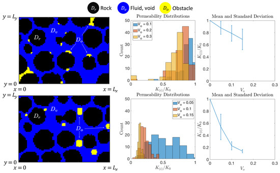
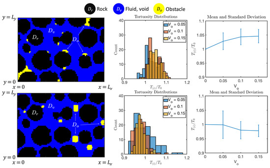
(Many-pore with CLPS model). We use the parameters with (21) model as in Table 3 for the many-pore example. We present the results for permeability in Figure 26. Additionally, we study the tortuosity as a function of obstruction volume, which we show in Figure 27. The case or corresponds to the increasing or decreasing average path lengths in the presence of obstructions.

Figure 26.
Flow properties with geometries created by CLPS in Example 4. Top row: pore-coating, and bottom row: pore-filling geometries. Left: example of with . Middle and right: experimental probability distribution of relative change in permeability for three values of .

Figure 27.
Transport properties with geometries created by CLPS in Example 4. Top row: pore-coating, and bottom row: pore-filling geometries. Left: example of with . Middle and right: experimental probability distribution of relative change in tortuosity for three values of .
We discuss these results here. We see good agreement between the single-pore, in Section 6.1), and many-pore cases. For pore-coating obstructions, there is a gradual decrease in permeability with , whereas, in the pore-filling case, the decrease in permeability is sharper. In the pore-filling case, the many-pore geometry with is, on average, more than twice as permeable as the single-pore case; see Table 5.
Next, from visual observations of geometries in Figure 27, we see for pore-coating featuring two instances of throat clogging and many small “colonies”. In addition, we see that is usually greater than in the unobstructed geometry; with a greater obstruction volume , there is a greater increase in . For pore-filling, we see tortuosity decreasing as increases.
6.3. Sensitivity of BN and Reduced Models CLPS and LP to Parameters
For any computational model, it is important to study its sensitivity to data. For models whose solutions depend on the data, a formal framework is provided, e.g., through Sobol indices [72] based on multivariate polynomial expansions of the quantity of interest; see, e.g., their use in [22]. This type of analysis requires high regularity of the quantities of interest so that the sensitivities, i.e., “derivatives”, can be assessed.
The quantities of interest in our models are (i) the geometries and (ii) the upscaled parameters such as .
For the first, (i) the framework to study (the smoothness of) their dependence on data is largely unavailable, while it loosely connects to the abstract framework of shape analysis in high-dimensional spaces. In the practical setting of this paper, our experiments indicate that the most important qualitative characteristic is whether the geometries produced by our models are of pore-coating or of pore-filling character, but it is unclear whether these observations can be correlated with some metrics that are to be studied quantitatively. Further analyses and theoretical framework are needed; see future work discussed in Section 7.
For (ii), the Darcy scale quantities rely on an averaging process carried out in upscaling, and thus can be believed to be reasonably smooth. However, the dependence of K resulting from DNS models and CLPS and LP models on their parameters raises formal challenges. One challenge is as follows: the permeability values K for some realizations of geometry can be zero because the associated geometries may include obstructions critically placed in the flow path. This feature may occur without any apparent dependence on the parameters of the simulations, and is an example of the non-smooth behavior of even the upscaled quantities.
At this time, we are unsure whether the formal framework of sensitivity applies to the quantities (i) and (ii) from our simulations. We comment on the qualitative observations only briefly.
6.3.1. Sensitivity of BN Models
In the DNS model for the pore-coating behavior related to the BN model for biofilm growth, the solutions governed by (12) and the pattern of depend on all the data to the PDE model. In particular in the results discussed here, we keep boundary conditions as well as the diffusion and reaction rates fixed using parameters from the literature; see [6,30].
In this paper, we vary the initial conditions through parameter and the right-hand-side function depending on parameter A. As we show in the geometries in Figure 8, and in the plots of permeabilities in Figure 14, the initial condition parameter for the DNS simulation plays a significant role in the biofilm growth pattern. For large(r) , the growth in biofilm is more evenly distributed near the walls, which results in more pronounced pore-coating behavior. For small , the attraction parameter A, when set to , contributes significantly to the “pore coating” pattern, and eventually results in the dependence of the upscaled quantities consistent with this pattern, as discussed in Remark 1. More detailed data for this sensitivity study are provided in Table 7.

Table 7.
Sensitivity of the probability distribution of to the simulation parameters and A for the geometries obtained with DNS for pore-coating scenarios. The values K presented here correspond to three selected vales of the relative volume from the set .
6.3.2. Sensitivity of reduced models CLPS and LP
For the reduced models CLPS and LP the control parameters include those discussed in Section 4 and Section 5. The CLPS model depends on parameters , as in Table 3, and the choice of is most delicate, as its small perturbations lead to different stationary solutions. The LP models solutions critically depend on as shown, e.g., in Table 4. The CLPS model is far more sensitive to its parameters than the LP model.
The choice of parameters for CLPS and LP is guided by heuristics, and the qualitative character of geometries is assessed by visual inspection. Most significantly, the reduced models produce geometries of drastically different characters (pore-coating or pore-filling) due to a small change in the control parameters, i.e., they produce bifurcations. This feature seems similar to the sensitivity of the Ising-like models of phase transitions to their critical parameters, such as the inverse temperature . We provide data for the sensitivity of the CLPS and LP models in Table 5 and Table 6.
Lastly, we provide an aggregated set of figures, which, taken together, illustrate the sensitivity of the simulation results to the initial conditions and to the initial geometry (single-pore or many-pore). See Figure 28, including our commentary on the overall sensitivity and qualitative and quantitative comparison between DNS, CLPS, LP and algebraic models.
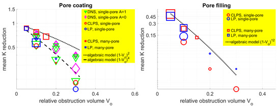
Figure 28.
Illustration of sensitivity of mean reduced permeability to the choice of and to the choice of initial pore geometry. The displayed results were obtained by DNS in various variants, and reduced models CLPS and LP for pore coating, and CLPS and LP for pore filling. The algebraic models guide the eye. The data are extracted from Table 6 and Table 7, and the marker size is proportional to the standard deviation for the data. The illustrations confirm the observations made in text, which we paraphrase here. The reduced model results generally qualitatively agree with DNS and algebraic models from Remark 1, but simulation models predict a more severe reduction in K than predicted by algebraic models. They have larger uncertainty for pore-coating scenarios and pore-filling scenarios for small . Predictions for single-pore and many-pore geometries are similar to each other for small , but their mean is not reliable at large due to clogging, especially for many-pore geometry.
In the end, we acknowledge the sensitivity to parameters, but do not see it as useful to study these quantitatively within formal frameworks which use differentiation or otherwise rely on the regularity of the quantities of interest. In turn, we believe more theoretical work is needed to study the metrics, smoothness, and overall sensitivity of the solutions on the model parameters.
6.4. Computational Complexity of BN and Comparison with Reduced Models CLPS and LP
The overall cost of each method, per realization , is the cost of each of
and has to be multiplied by the number I of realizations.
In the estimates below, we assume we have M grid cells, including those in . However, an efficient implementation may have lower complexity or be based on rather than M, depending on how we handle the keyed-out elements from . Regardless, we have for single-pore and many-pore geometries in . For large-case simulations in , which are not reported here, typically, .
We report the cost of the algorithms, which create one realization of . The pre-processing cost involves the initialization of algorithms with some initial conditions, which use a random number generator called I times on a vector of size M.
Throughout, we denote the cost of solving a linear system with M unknowns by . We recall that the cost of direct methods such as LU and QR in the MATLAB environment for dense matrices is with . On the other hand, the discretizations we consider lead to sparse linear systems, and it is well known that appropriate direct and iterative solvers have a cost of , where p is band size. On the other hand, the solver in the post-processing environment HybGE-Flow3D has , since it uses state-of-the-art preconditioners, and in , the band size .
Once are found, we post-process. The cost of post-processing and upscaling to Darcy scale properties is about .
In general, we find that the cost of generation of far outweighs that of post-processing for DNS and CLPS, and is comparable to that for LP. The DNS of BN seems feasible for , but may be unfeasible for .
Moreover, we find that the cost of data storage and file IO is already considerable for , and may require creative approaches when .
6.4.1. Complexity of BN
The solver BN for DNS requires the solution of two coupled nonlinear PDEs for , each of size M. Additionally, we keep track of and update the Lagrange multiplier, also of size M. In other words, we have unknowns: . We also pre-compute prior to simulations.
We solve the problem over 100 to 1000 time-steps, depending on the case, and each requires, on average, about two iterations of the semi-implicit method. We require around operations per iteration, plus the cost . The former include computing diffusion coefficients, the Jacobian, residuals, and other operations. For the linear solver, the system is sparse but not symmetric.
We provide approximate times to indicate complexity when solving BN up until plugging. We report on wall clock time on a Linux multicore desktop with MATLAB. For single-pore geometry with , this took about for and for . For many-pore geometry with , this took for and for . These times simply indicate that it takes longer to simulate until complete plugging when the obstructions adhere more closely to the walls.
6.4.2. Complexity of CLPS
As compared to BN, the CLPS algorithm only solves one variable , and uses linear symmetric non-degenerate diffusion and time-lagging, without any additional iterations. The localization functions are pre-computed. Thanks to these reductions, the complexity is considerable compared to BN.
The cost per time-step is about operations, which icludes dealing with the volume constraint plus the cost of the linear solver . We run time-steps until a stationary solution is found, which ranges from 100 to .
Depending on the case, single-pore simulations run for about on average.
6.4.3. Complexity of LP
The LP algorithm might take as many as time-steps to reach the stationary solution, but each is very inexpensive, and requires only the cost of swaps and recalculation of Hamiltonian update . We approximate this cost to be 10 operations per time-step.
Depending on the case, LP simulations for single-pore on a laptop take less than on average, and are about 6 times faster than CLPS.
7. Summary and Future Work
Imaging and other high-resolution data pose an opportunity and, simultaneously, a challenge to computational science. In this paper, our focus is on pore-scale data for flow and transport, and their upscaling to Darcy-scale properties of porous media, such as permeability and tortuosity. Specifically, we consider a medium which changes due to clogging, with two patterns of obstructions in pore-scale geometries, referred to as pore-coating and pore-filling. Both are motivated by their important applications to biofilm and hydrate crystal growth, respectively.
Interpreting the static imaging data as grids for flow simulations and upscaling is possible. However, imaging of pore-scale which changes in time due to clogging poses additional difficulties, and handling the potentially large collection of geometries is extremely computationally intensive, and requires calibration and tuning. Using DNS for time-dependent processes instead of imaging is quite complex and comes with considerable uncertainty.
In this paper, we presented an alternative reduced model, which can create off-line probability distributions of properties of interest without the DNS. In particular, we present two algorithms which generate plausible geometries with obstructions called , which clog the pores. These algorithms are not simulations of the actual physical process, but rather simulate the presence of which appear similar to those observed in experiments. The methods have roots in mathematical and statistical models of phase separation; they are easily tunable and efficient.
In the paper, we demonstrated that our reduced models produce comparable results to those of DNS, both by visual inspection of and when considering the upscaled quantities. Overall, the CLPS model is about one order of magnitude more efficient than DNS, and the LP model is about one further order of magnitude more efficient than CLPS. However, as we move from DNS to CLPS to LP models, we also move farther and farther away from the actual physical model of generating obstructions.
More work is needed to understand this trend and how to use and calibrate efficient reduced models which maintain close agreement with physical simulations. At the same time, validation efforts are needed to further calibrate the DNS models, which can serve as the basis for reduced models. In addition, theoretical analyses, and, specifically, new metrics, are needed to compare the images we generate with reduced models to the DNS and to the imaging data. In this paper, we used judgement made by the human eye, but we are currently exploring various emerging data science approaches which can be used to analyze the similarity between shapes.
Finally, we aim to continue the validation efforts of the probability distributions we generate with the experimentally obtained Darcy-scale quantities. In particular, in this paper, we considered only two representative geometries, called single-pore and many-pore. Further testing and validation efforts should include testing the reduced models in a collection of pore geometries ranging from simple to complicated. Since the permeability depends very much on the local arrangement of the pores and throats, it depends not just on the size but also on the choice of an REV, and this randomness is even more pronounced when the geometry is modified by reactive transport starting from random initial conditions. These facts motivate this paper, since reduced models would produce more reliable results than, say, algebraic formulas, such as those in Remark 1; we observed this fact in [6].
We believe that it would be useful to create a library of probability distributions corresponding to the obstructed domains classified by type, say, channel-like, or large porosity (glass-beads), or sand-stone geometries. These efforts may be connected to some theoretical analyses of shapes, which we hope to address in the future.
Our current work also includes further calibration of the models to discover the optimal values of parameters for CLPS and LP starting from the available data. In this direction, we plan to explore data science approaches. There are also many interesting application-specific challenges, including the dependence of the results on I, the size and the shape of the rock domain in the selected REV, and the voxel resolution h.
Author Contributions
Conceptualization: M.P., J.U. and C.S.; investigation: J.U and C.S.; software: J.U., C.S. and M.P.; writing—original draft preparation: M.P., J.U. and C.S.; supervision: M.P. All authors have read and agreed to the published version of the manuscript.
Funding
This research was partially supported by the grants from National Science Foundation DMS-1522734 “Phase transitions in porous media across multiple scales” (with supplement DMS-1738014), as well as by NSF DMS-1912938 “Modeling with Constraints and Phase Transitions in Porous Media”. Choah Shin would like to thank Larry Martin and Joyce O’Neill for their generous support with the endowed College of Science at Oregon State fellowship 2019–2020. This material is also based upon work supported by, and while serving at, the National Science Foundation: M. Peszynska was supported by NSF IRD plan 2019-21.
Institutional Review Board Statement
Not applicable.
Informed Consent Statement
Not applicable.
Acknowledgments
The authors would like to thank the anonymous referees whose comments helped to improve the exposition. The bulk of J. Umhoefer’s work was completed while he was a PhD student at Oregon State University [50]. This material is based upon work partially supported by, and while serving at, the National Science Foundation. Any opinion, findings, and conclusions or recommendations expressed in this material are those of the authors and do not necessarily reflect the views of the National Science Foundation. We also want to thank our former collaborators and co-authors in [6] for the inspiration and access to data.
Conflicts of Interest
The authors declare no conflict of interest.
Appendix A
Appendix A.1. Numerical Scheme for CLPS
Numerical solution of gradient flow problems such as Allen–Cahn equations, such as those in Section 4, is challenging, and the literature is abundant. The first challenge is the presence of sharp fronts, which require a fine spatial grid and delicate time-stepping. The second challenge is the strong nonlinearity without monotonicity; this feature has motivated the construction of various semi-implicit schemes which provable stability in a specially chosen quantity of interest which can be obtained. We refer, e.g., to [57,58].
In this paper, for the spatial discretization of (21), we apply a cell-centered finite-difference scheme. For time discretization, we apply an Implicit–Explicit scheme. We treat the linear terms, such as diffusion terms, implicitly in time, and we treat nonlinear terms explicitly in time. For problems with constraints, we also implicitly solve . We keep the time-step small to maintain accuracy, but the explicit treatment of nonlinearities makes the system very easy to implement. The linear systems are solved by a direct solver in MATLAB.
Appendix A.2. Illustrations of CLPS Model in 1d
We consider the evolution problem (21) in 1d, with and . We set up examples to illustrate the role of parameters and . We use . To demonstrate the effect of localization as in (21e), considering , we define the continuous piecewise linear with and , for this example only.
We use a family of random initial conditions for which the pointwise values are drawn from the uniform distribution. For each, we find the corresponding stationary solutions .
Our first example shows that different initial conditions give different stationary solutions.
Example A1.
We set , and and approximate the solutions to (21). We let the solution evolve until the time , after which the solutions remain essentially stationary. In Figure A1, we show the two stationary states corresponding to i = 1 and i = 2. In Figure A2, we illustrate the well-known impact of parameter ϵ, when the initial state , and .
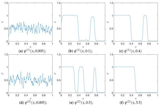
Figure A1.
Solutions to Example A1, corresponding to with (top) and (bottom) at three different times t. The right column is at , different for each i.

Figure A2.
Solutions in Example A1, showing the impact of the coefficient . From left to right, , with the corresponding .
Next, we study the impact of the parameter and of the localization functions.
Example A2.
We set and , and consider or . In Figure A3, we confirm that a positive θ encourages near . At the same time, away from Γ, the function competes with . With large enough , the behavior is dominated by , resulting in away from . With , we obtain , but with , the impact of localisation prevails over and we obtain .
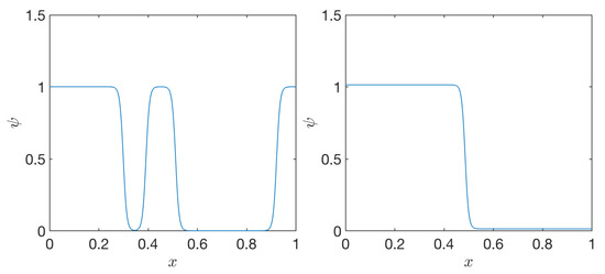
Figure A3.
The solutions from Ex. A2 showing the impact of the coefficient . From left to right: with , respectively.
Appendix A.3. Numerical Approximation to Stokes Flow
We approximate the solutions to the Stokes flow problem from Section 2.3 with a computational model built on the MAC scheme and implemented in MATLAB and in solver HybGe-Flow3D [16]. The approximations pressure and velocity values are given on a staggered voxel grid, with the pressures given as cell-centered quantities, the -velocity component given on the left and right edges of a cell and the -component velocity values given on the bottom and top edges. The additional feature of our implementation is that it is very efficient when handling a collection of obstruction volumes; the method follows the stochastic immersed volume approach described in detail in [16].
References
- Bear, J.; Cheng, A.H.-D. Modeling Groundwater Flow and Contaminant Transport; Springer: Berlin/Heidelberg, Germany, 2010. [Google Scholar]
- Zhang, D. Stochastic Methods for Flow in Porous Media: Coping with Uncertainties; Elsevier: Amsterdam, The Netherlands, 2001. [Google Scholar]
- Ossiander, M.; Peszynska, M.; Madsen, L.; Mur, A.; Harbert, W. Estimation and simulation for geospatial porosity and permeability data. Environ. Ecol. Stat. 2017, 24, 109–130. [Google Scholar] [CrossRef]
- Ossiander, M.; Peszynska, M.; Vasylkivska, V. Conditional stochastic simulations of flow and transport with karhunen-loeve expansions, stochastic collocation, and sequential gaussian simulation. J. Appl. Math. 2014, 2014, 21. [Google Scholar] [CrossRef]
- Ganis, B.; Klie, H.; Wheeler, M.F.; Wildey, T.; Yotov, I.; Zhang, D. Stochastic collocation and mixed finite elements for flow in porous media. Comput. Methods Appl. Mech. Eng. 2008, 197, 3547–3559. [Google Scholar] [CrossRef]
- Peszynska, M.; Trykozko, A.; Iltis, G.; Schlueter, S.; Wildenschild, D. Biofilm growth in porous media: Experiments, computational modeling at the porescale, and upscaling. Adv. Water Resour. 2016, 95, 288–301. [Google Scholar] [CrossRef]
- Peszynska, M.; Trykozko, A. Pore-to-core simulations of flow with large velocities using continuum models and imaging data. Comput. Geosci. 2013, 17, 623–645. [Google Scholar] [CrossRef]
- Trykozko, A.; Peszynska, M.; Dohnalik, M. Modeling non-Darcy flows in realistic porescale proppant geometries. Comput. Geotech. 2015, 71, 352–360. [Google Scholar] [CrossRef]
- Kim, D.; Peters, C.A.; Lindquist, W.B. Upscaling geochemical reaction rates accompanying acidic co2-saturated brine flow in sandstone aquifers. Water Resour. Res. 2011, 47. [Google Scholar] [CrossRef]
- Blunt, M.J. Flow in porous media—Pore-network models and multiphase flow. Curr. Opin. Colloid Interface Sci. 2001, 6, 197–207. [Google Scholar] [CrossRef]
- Porter, M.L.; Wildenschild, D. Image analysis algorithms for estimating porous media multiphase flow variables from computed microtomography data: A validation study. Comput. Geosci. 2010, 14, 15–30. [Google Scholar] [CrossRef]
- Kulkarni, R.; Tuller, M.; Fink, W.; Wildenschild, D. Three-dimensional multiphase segmentation of x-ray CT data of porous materials using a Bayesian Markov random field framework. Vadose Zone J. 2012, 11. [Google Scholar] [CrossRef]
- Digital Rocks Portal. Available online: https://www.digitalrocksportal.org/ (accessed on 1 January 2020).
- Prodanović, M.; Mehmani, A.; Sheppard, A.P. Imaged-based multiscale network modelling of microporosity in carbonates. Geol. Soc. Lond. Spec. Publ. 2015, 406, 95–113. [Google Scholar]
- Balhoff, M.T.; Thompson, K.E.; Hjortsø, M. Coupling pore-scale networks to continuum-scale models of porous media. Comput. Geosci. 2007, 33, 393–410. [Google Scholar] [CrossRef]
- Costa, T.B.; Kennedy, K.; Peszynska, M. Hybrid three-scale model for evolving pore-scale geometries. Comput. Geosci. 2018, 22, 925–950. [Google Scholar] [CrossRef]
- Torquato, S.; Haslach, H.W., Jr. Random heterogeneous materials: Microstructure and macroscopic properties. Appl. Mech. Rev. 2002, 55, B62–B63. [Google Scholar] [CrossRef]
- Peszynska, M.; Trykozko, A.; Sobieski, W. Forchheimer law in computational and experimental studies of flow through porous media at porescale and mesoscale. Math. Sci. Appl. 2010, 32, 463–482. [Google Scholar]
- Peszynska, M.; Trykozko, A.; Augustson, K. Computational upscaling of inertia effects from porescale to mesoscale. In Proceedings of the International Conference on Computational Science, Baton Rouge, LA, USA, 25–27 May 2009; Allen, G., Nabrzyski, J., Seidel, E., van Albada, D., Dongarra, J., Sloot, P., Eds.; Springer: Berlin/Heidelberg, Germany, 2009; pp. 695–704. [Google Scholar]
- Peszynska, M.; Trykozko, A. Convergence and stability in upscaling of flow with inertia from porescale to mesoscale. Int. J. Multiscale Comput. Eng. 2011, 9, 215–229. [Google Scholar] [CrossRef]
- Coyte, K.Z.; Tabuteau, H.; Gaffney, E.A.; Foster, K.R.; Durham, W.M. Microbial competition in porous environments can select against rapid biofilm growth. Proc. Natl. Acad. Sci. USA 2017, 114, E161–E170. [Google Scholar] [CrossRef] [PubMed]
- Landa-Marbán, D.; Liu, N.; Pop, I.S.; Kumar, K.; Pettersson, P.; Bødtker, G.; Skauge, T.; Radu, F.A. A pore-scale model for permeable biofilm: Numerical simulations and laboratory experiments. Transp. Porous Media 2019, 127, 643–660. [Google Scholar] [CrossRef]
- Chu, J.; Engquist, B.; Prodanovic, M.; Tsai, R. A multiscale method coupling network and continuum models in porous media. ii. Single-and two-phase flows. In Advances in Applied Mathematics, Modeling, and Computational Science; Springer: Berlin/Heidelberg, Germany, 2013; pp. 161–185. [Google Scholar]
- Quarteroni, A.; Manzoni, A.; Negri, F. Reduced Basis Methods for Partial Differential Equations: An Introduction; Springer: Berlin/Heidelberg, Germany, 2015; Volume 92. [Google Scholar]
- Peherstorfer, B.; Willcox, K.; Gunzburger, M. Survey of multifidelity methods in uncertainty propagation, inference, and optimization. SIAM Rev. 2018, 60, 550–591. [Google Scholar] [CrossRef]
- Thullner, M.; Zeyer, J.; Kinzelbach, W. Influence of microbial growth on hydraulic properties of pore networks. Transp. Porous Media 2002, 49, 99–122. [Google Scholar] [CrossRef]
- Liu, X.; Flemings, P.B. Dynamic multiphase flow model of hydrate formation in marine sediments. J. Geophys. Res. 2008, 112, B03101. [Google Scholar] [CrossRef]
- Lake, L.W. Enhanced oil Recovery; Prentice Hall: Denver, CO, USA, 1989. [Google Scholar]
- Prodanovic, M.; Esteva, M.; Hanlon, M.; Nanda, G.; Agarwal, P. Digital Rocks Portal: A repository for porous media images. In AGU Fall Meeting Abstracts; 2015; p. MR43A-02. [Google Scholar]
- Shin, C.; Alhammali, A.; Bigler, L.; Vohra, N.; Peszynska, M. Coupled flow and biomass-nutrient growth at pore-scale with permeable biofilm, adaptive singularity and multiple species. Math. Biosci. Eng. 2021, in press. [Google Scholar]
- Peszynska, M.; Hong, W.-L.; Torres, M.E.; Kim, J.-H. Methane Hydrate Formation in Ulleung Basin Under Conditions of Variable Salinity: Reduced Model and Experiments. Transp. Porous Media 2016, 114, 1–27. [Google Scholar] [CrossRef]
- Peszynska, M.; Showalter, R.; Webster, J. Advection of methane in the hydrate zone: Model, analysis and examples. Math. Methods Appl. Sci. 2015, 38, 4613–4629. [Google Scholar] [CrossRef]
- Peszynska, M.; Medina, F.P.; Hong, W.; Torres, M.E. Reduced numerical model for methane hydrate formation under conditions of variable salinity. time-stepping variants and sensitivity. Computation 2015, 4, 1. [Google Scholar] [CrossRef]
- Ebigbo, A.; Phillips, A.; Gerlach, R.; Helmig, R.; Cunningham, A.B.; Class, H.; Spangler, L.H. Darcy-scale modeling of microbially induced carbonate mineral precipitation in sand columns. Water Resour. Res. 2012, 48. [Google Scholar] [CrossRef]
- Tang, Y.; Valocchi, A.J.; Werth, C.J. A hybrid pore-scale and continuum-scale model for solute diffusion, reaction, and biofilm development in porous media. Water Resour. Res. 2015, 51, 1846–1859. [Google Scholar] [CrossRef]
- Verba, C.; Thurber, A.; Alleau, Y.; Koley, D.; Peszynska, M.; Colwell, F.; Torres, M. Feasibility of Biogeochemical Sealing of Wellbore Cements: Lab and Simulation Tests; U.S. Department of Energy, National Energy Technology Laboratory: Albany, OR, USA, 2017.
- Verba, C.; Thurber, A.R.; Alleau, Y.; Koley, D.; Colwell, F.; Torr, M.E. Mineral changes in cement-sandstone matrices induced by biocementation. Int. J. Greenh. Gas Control 2016, 49, 312–322. [Google Scholar] [CrossRef]
- Baveye, P.; Valocchi, A. An evaluation of mathematical models of the transport of biologically reacting solutes in saturated soils and aquifers. Water Resour. Res. 1989, 25, 1413–1421. [Google Scholar] [CrossRef]
- Molz, F.J.; Widdowson, M.A.; Benefield, L.D. Simulation of Microbial Growth Dynamics Coupled to Nutrient and Oxygen Transport in Porous Media. Water Resour. Res. 1986, 22, 1207–1216. [Google Scholar] [CrossRef]
- Soleimani, S.; Geel, P.J.V.; Isgor, O.B.; Mostafa, M.B. Modeling of biological clogging in unsaturated porous media. J. Contam. Hydrol. 2009, 106, 39–50. [Google Scholar] [CrossRef] [PubMed]
- Chen, X.; Espinoza, D.N. Ostwald ripening changes the pore habit and spatial variability of clathrate hydrate. Fuel 2018, 214, 614–622. [Google Scholar] [CrossRef]
- Ruppel, C.D.; Kessler, J.D. The interaction of climate change and methane hydrates. Rev. Geophys. 2017, 55, 126–168. [Google Scholar] [CrossRef]
- Solomon, S.; Qin, D.; Manning, M.; Chen, Z.; Marquis, M.; Averyt, K.B.; Tignor, M.; Miller, H.L. Climate Change 2007: The Physical Science Basis; Technical Report; Cambridge University Press: Cambridge, UK, 2007. [Google Scholar]
- Zhang, L.; Yang, L.; Liu, Y.; Song, Y. Microstructural characteristics of natural gas hydrates hosted in various sand sediments. Phys. Chem. Chem. Phys. 2015, 17, 22632–22641. [Google Scholar]
- Kumar, A.; Maini, B.; Bishnoi, P.R.; Clarke, M.; Zatsepina, O.; Srinivasan, S. Experimental determination of permeability in the presence of hydrates and its effect on the dissociation characteristics of gas hydrates in porous media. J. Pet. Sci. Eng. 2010, 70, 114–122. [Google Scholar] [CrossRef]
- Huang, D.; Fan, S. Thermal conductivity of methane hydrate formed from sodium dodecyl sulfate solution. J. Chem. Eng. Data 2004, 49, 1479–1482. [Google Scholar] [CrossRef]
- Spangenberg, E. Modeling of the influence of gas hydrate content on the electrical properties of porous sediments. J. Geophys. Res. Solid Earth 2001, 106, 6535–6548. [Google Scholar] [CrossRef]
- Tegze, G.; Pusztai, T.; Tóth, G.; Gránásy, L.; Svandal, A.; Buanes, T.; Kuznetsova, T.; Kvamme, B. Multiscale approach to CO2 hydrate formation in aqueous solution: Phase field theory and molecular dynamics. nucleation and growth. J. Chem. Phys. 2006, 124, 234710. [Google Scholar] [CrossRef] [PubMed]
- Kvamme, B.; Graue, A.; Aspenes, E.; Kuznetsova, T.; Gránásy, L.; Tóth, G.; Pusztai, T.; Tegze, G. Kinetics of solid hydrate formation by carbon dioxide: Phase field theory of hydrate nucleation and magnetic resonance imaging. Phys. Chem. Chem. Phys. 2004, 6, 2327–2334. [Google Scholar] [CrossRef]
- Umhoefer, J. Modeling Flow and Transport at Pore Scale with Obstructions. Ph.D. Thesis, Oregon State University, Corvallis, OR, USA, 2019. [Google Scholar]
- Costa, T. HybGe-Flow3d. Available online: https://github.com/numsol/HybGe-Flow3D (accessed on 1 January 2021).
- Noorden, T.L.V.; Pop, I.S. A Stefan problem modelling crystal dissolution and precipitation. IMA J. Appl. Math. 2008, 73, 393–411. [Google Scholar] [CrossRef][Green Version]
- Clennell, M.B. Tortuosity: A guide through the maze. Geol. Soc. Lond. Spec. Publ. 1997, 122, 299–344. [Google Scholar] [CrossRef]
- LeVeque, R.J. Finite Volume Methods for Hyperbolic Problems; Cambridge Texts in Applied Mathematics; Cambridge University Press: Cambridge, UK, 2002. [Google Scholar]
- Frederick, M.R.; Kuttler, C.; Hense, B.A.; Eberl, H.J. A mathematical model of quorum sensing regulated eps production in biofilm communities. Theor. Biol. Med Model. 2011, 8, 1–29. [Google Scholar] [CrossRef] [PubMed]
- Visintin, A. Models of phase transitions. In Progress in Nonlinear Differential Equations and their Applications, 28; Birkhäuser Boston Inc.: Boston, MA, USA, 1996. [Google Scholar]
- Shen, J.; Yang, X. Numerical approximations of Allen-Cahn and Cahn-Hilliard equations. Discret. Contin. Dyn. Syst. 2010, 28, 1669–1691. [Google Scholar] [CrossRef]
- Elliott, C.M.; Stuart, A.M. The Global Dynamics of Discrete Semilinear Parabolic Equations. SIAM J. Numer. Anal. 1993, 30, 1622–1663. [Google Scholar] [CrossRef]
- Rockafellar, R.T. Lagrange Multipliers and Optimality. SIAM Rev. 1993, 35, 183–238. [Google Scholar] [CrossRef]
- Rubinstein, J.; Sternberg, P. Nonlocal reaction—Diffusion equations and nucleation. IMA J. Appl. Math. 1992, 48, 249–264. [Google Scholar] [CrossRef]
- Frank, F.; Ray, N.; Knabner, P. Numerical investigation of homogenized stokes—Nernst—Planck—Poisson systems. Comput. Vis. Sci. 2011, 14, 385–400. [Google Scholar] [CrossRef]
- Ray, N.; Muntean, A.; Knabner, P. Rigorous homogenization of a stokes-nernst-planck-poisson system. J. Math. Anal. Appl. 2012, 390, 374–393. [Google Scholar] [CrossRef]
- Herz, M.; Ray, N.; Knabner, P. Existence and uniqueness of a global weak solution of a Darcy-Nernst-Planck-Poisson system. GAMM-Mitteilungen 2012, 35, 191–208. [Google Scholar] [CrossRef]
- Oono, Y.; Puri, S. Study of phase-separation dynamics by use of cell dynamical systems. I. Modeling. Phys. Rev. A 1988, 38, 434–453. [Google Scholar] [CrossRef]
- Puri, S.; Oono, Y. Study of phase-separation dynamics by use of cell dynamical systems. II. Two-dimensional demonstrations. Phys. Rev. A 1988, 38, 1542–1565. [Google Scholar] [CrossRef] [PubMed]
- Metropolis, N.; Rosenbluth, A.W.; Rosenbluth, M.N.; Teller, A.H.; Teller, E. Equation of state calculations by fast computing machines. J. Chem. Phys. 1953, 21, 1087–1092. [Google Scholar] [CrossRef]
- Madras, N.N. Lectures on Monte Carlo Methods; American Mathematical Soc.: Providence, RI, USA, 2002. [Google Scholar]
- Shonkwiler, R.W.; Mendivil, F. Explorations in Monte Carlo Methods; Springer Science & Business Media: New York, NY, USA, 2009. [Google Scholar]
- Sarkisov, L.; Monson, P.A. Modeling of adsorption and desorption in pores of simple geometry using molecular dynamics. Langmuir 2001, 17, 7600–7604. [Google Scholar] [CrossRef]
- Sarkisov, L.; Monson, P.A. Lattice model of adsorption in disordered porous materials: Mean-field density functional theory and Monte Carlo simulations. Phys. Rev. E 2002, 65, 011202. [Google Scholar] [CrossRef] [PubMed]
- Medina, F.P.; Peszynska, M. Hybrid modeling and analysis of multicomponent adsorption with applications to coalbed methane. In Porous Media: Theory, Properties, and Applications; Nova Science Publishers: Hauppauge, NY, USA, 2016; pp. 1–52. ISBN 978-1-63485-474-0. [Google Scholar]
- Sobol, I.M. Global sensitivity indices for nonlinear mathematical models and their monte carlo estimates. Math. Comput. Simul. 2001, 55, 271–280. [Google Scholar] [CrossRef]
Publisher’s Note: MDPI stays neutral with regard to jurisdictional claims in published maps and institutional affiliations. |
© 2021 by the authors. Licensee MDPI, Basel, Switzerland. This article is an open access article distributed under the terms and conditions of the Creative Commons Attribution (CC BY) license (http://creativecommons.org/licenses/by/4.0/).