Optimization of the Controls against the Spread of Zika Virus in Populations

Abstract

In this paper, we study and explore two control strategies to decrease the spread of Zika virus in the human and mosquito populations. The control strategies that we consider in this study are awareness and spraying campaigns. We solve several optimal control problems relying on a mathematical epidemic model of Zika that considers both human and mosquito populations. The first control strategy is broad and includes using information campaigns, encouraging people to use bednetting, wear long-sleeve shirts, or similar protection actions. The second control is more specific and relies on spraying insecticides. The control system relies on a Zika mathematical model with control functions. To develop the optimal control problem, we use Pontryagins’ maximum principle, which is numerically solved as a boundary value problem. For the mathematical model of the Zika epidemic, we use parameter values extracted from real data from an outbreak in Colombia. We study the effect of the costs related to the controls and infected populations. These costs are important in real life since they can change the outcomes and recommendations for health authorities dramatically. Finally, we explore different options regarding which control measures are more cost-efficient for society.

1. Introduction

The Zika virus is primarily spread by the female Aedes aegypti mosquito, which must feed on blood to lay eggs. The virus can cause symptoms such as fever, red eyes, joint pain, headache, and a maculopapular rash [1]. A pregnant woman infected by ZIKV can have had vertical transmission to the fetus, which increases the risk of microcephaly. Therefore, the control and eradication of ZIKV are crucial due to the social impact of the disease from different perspectives.

The infection caused by ZIKV is a significant vector-transmitted disease, which in the last few decades caused many cases in Latin America [2]. Moreover, the ZIKV virus has spread worldwide in countries such as Australia, Canada, France, Italy, and Spain. For instance, in the USA, the state of Florida reported over 735 travel-related Zika cases since February 2016, becoming the first state in the continental USA to report multiple laboratory-confirmed autochthonous cases of Zika [3]. Based on the previous facts, it makes sense to develop studies to decide how we can slow down or eradicate the spread of the ZIKV. In this study, we consider an optimal control design considering the cost-effectiveness of strategies to accomplish the aims mentioned above. We use a previously developed mathematical model along with objective functions that help us to reach the purpose of the study. The outcomes of this approach can lead health authorities to make the most convenient decisions regarding the slowing down of the transmission of the ZIKV, considering some cost associate with different choices.

In this study, we use a mathematical model for the ZIKV transmission using a system of nonlinear differential equations. The model includes the populations of humans and mosquitoes. In the mathematical model, the birth rate of the mosquitoes is assumed to be equal to their death rate, and the same is assumed between birth and death rates for humans [2]. Moreover, the model considers a hundred percent vertical transmission in the human population. Furthermore, the model includes mutations of the ZIKV; therefore, the recovered subpopulation can return to the susceptible state [2,4,5]. This type of mathematical modeling approach is used widely to study the dynamics of diseases in populations [6,7]. As mentioned above, there is a variety of mathematical models for ZIKV transmission. We did not consider very detailed mathematical models that include mosquito larvae, since then the parameters are not very easily identifiable and our aim here is to propose an approach to study the effects of control policies with a classical ZIKV model.

A critical feature of this type of epidemiological models is the basic reproduction number ${\mathcal{R}}_0$ [6,8]. This famous number, which is currently used to characterize the COVID-19 pandemic, is defined as the expected number of new infections from one infected individual in a fully susceptible population through the entire duration of the infectious period. In this work, we use parameter values that were estimated using real data from Colombia [2].

Some previous interesting publications use optimal control techniques to minimize the spread of the diseases in the presence of vectors such as mosquitoes [9,10,11,12,13]. In particular, in [10] the authors considered an asymptotic carrier, which might be an important factor in the dynamics. Saturation and optimal controls were considered and studied in [9]. In [14], the authors studied the optimal effects of bednets (prevention), treatments of infective, and spray of insecticides on the disease spread. The authors use Pontryagins’ Maximum Principle to determine the necessary conditions to control ZIKV. The authors used a particular model which assumed an effective contact rate between infected and susceptible humans could result in infection. Moreover, the authors included the infected and exposed populations for humans and mosquitoes in the objective functional $\mathcal{J}$. Among other results, they found that exposed mosquitoes are not affected by the prevention and treatment controls. Surprisingly, prevention and insecticide control increased the number of infected humans [14]. Furthermore, they found that treatment and insecticide spraying controls increased the number of exposed and infected humans despite the fact that the infected and exposed human populations are included in the objective functional $\mathcal{J}$. In our study, we include two time-dependent controls (prevention and insecticide), and only the infected populations for humans and mosquitoes in the objective functional $\mathcal{J}$.

Here, we use Pontryagins’ maximum principle in order to solve the optimal control. Thus, we can find the conditions that are necessary for the Zika disease to be controlled optimally. The outcome of the optimal control problem is the particular time-dependent controls related to the Zika mathematical model. In addition, we can observe the new dynamics under the action of time-dependent controls. It is important to remark that various studies regarding optimal control do not mention the paramount importance of the costs related to the controls and infected populations. These costs can change dramatically the outcomes and recommendations made by health authorities. In fact, assigning costs to infected populations is not an easy task and may involve ethical, political, philosophical, and sanitary considerations in many cases. Nowadays cost-effectiveness analysis has become a common method to use for decision making [15,16,17,18]. There are several studies that have estimated the associated costs of control policies and infected individuals [19,20,21,22,23,24].

This paper is organized as follows. In Section 2, we present the Zika mathematical model and introduce the time-dependent controls. In Section 3, we present the objective functional $\mathcal{J}$. Moreover, we also construct the optimality system using Pontryagins’ maximum principle and explain the procedure to solve the control problem. In Section 4, we numerically solve the control problem and discuss the outcomes. Finally, in Section 5, we present the conclusions and discussion.

2. Mathematical Model

The mathematical model that we use in this study for the Zika virus transmission relies on a system of nonlinear differential equations. The model includes the populations of humans and mosquitoes. For more details, see [2]. A crucial characteristic of the model is that it considers vertical transmission in the human population. In addition, the model includes mutations of the ZIKV, therefore the recovered individuals can return to the susceptible state [2,4,5]. The Zika virus spreads by the effective contact between an infected mosquito with a susceptible individual and vice-versa. This effective contact depends on several environmental factors such as weather, temperature, altitude, clothes, bednets, and mosquito bite rate [3,25,26,27]. Varying these factors would generate different outcomes of transmission of the disease.

The mathematical model comprises five ordinary differential equations. Thus, we have a continuous mathematical model for the transmission and evolution of the Zika virus in human and mosquito populations. The total population of human $N_h\left(t\right)$ is divided into three subpopulations: Humans who may become infected (Susceptible $S_h\left(t\right)$), humans infected by the Zika virus (Infected $I_h\left(t\right)$) and humans who have recovered from Zika virus (Recovered $R_h\left(t\right)$) [2]. Parameter $b_h$ is the human birth rate. This birth rate $b_h$ is assumed as equal to that of natural death $d_h$. The total population of mosquitoes $N_T\left(M\right)$ is divided in two subpopulations: Mosquitoes which may become infected $S_M\left(t\right)$ and mosquitoes infected by the Zika virus $I_M\left(t\right)$. Parameters $b_M$ and $d_M$ are the birth and death rates respectively. A susceptible human can transit to the infected subpopulation $I_h\left(t\right)$ because of an effective transmission due to being bitten by an infected mosquito depending on parameter ${\beta }_h$. A susceptible mosquito can be infected if there is an effective transmission when it stings an infected human depending on the parameter ${\beta }_M$. We assume a hundred percent vertical transmission in the human population. A fraction Ψ of the recovered humans may return to the susceptible state. Finally, homogeneous mixing is assumed, i.e., all susceptible humans have the same probability of being infected and all susceptible mosquitoes have the same probability of infection. Using these ideas and the structure of mathematical modeling in epidemiology we have the following model [2]:

$$\begin{array}{ccc}\hfill S_h^{\prime }\left(t\right)& =& R_h\left(t\right)(b_h+\mathsf{\Psi })-{\beta }_h{S}_h\left(t\right){\displaystyle \frac{I_M\left(t\right)}{N_h\left(t\right)}},\hfill \\ \hfill I_h^{\prime }\left(t\right)& =& {\beta }_h{S}_h\left(t\right){\displaystyle \frac{I_M\left(t\right)}{N_h\left(t\right)}}-\mathsf{\Lambda }{I}_h\left(t\right),\hfill \\ \hfill R_h^{\prime }\left(t\right)& =& \mathsf{\Lambda }{I}_h\left(t\right)-R_h\left(t\right)(\mathsf{\Psi }+d_h),\hfill \\ \hfill S_M^{\prime }\left(t\right)& =& b_M{N}_M\left(t\right)-{\beta }_M{S}_M\left(t\right){\displaystyle \frac{I_h\left(t\right)}{N_h\left(t\right)}}-d_M{S}_M\left(t\right),\hfill \\ \hfill I_M^{\prime }\left(t\right)& =& {\beta }_M{S}_M\left(t\right){\displaystyle \frac{I_h\left(t\right)}{N_h\left(t\right)}}-d_M{I}_M\left(t\right).\hfill \end{array}$$

(1)

If we add all the human classes, one gets, $N_h^{\prime }\left(t\right)=S_h^{\prime }\left(t\right)+I_h^{\prime }\left(t\right)+R_h^{\prime }\left(t\right)=0$ therefore the human population is constant. Adding the susceptible and infected vector subpopulations one gets, $N_M^{\prime }\left(t\right)=S_M^{\prime }\left(t\right)+I_M^{\prime }\left(t\right)=b_M{N}_M\left(t\right)-d_M{N}_M\left(t\right)$. System (1) is well-posed, in the sense that if the initial data $(S_h\left(t\right),I_h\left(t\right),R_h\left(t\right),S_M\left(t\right),I_M\left(t\right))$ are in the region ${\mathbb{R}}_{+}^5$, then they will be defined for all time $t\ge 0$ and remain in ${\mathbb{R}}_{+}^5$. Initial conditions are given by $(S_h\left(0\right),I_h\left(0\right),R_h\left(0\right),S_M\left(0\right),I_M\left(0\right))$.

Notably, other models have been presented to study the spread of Zika in human and mosquito populations. However, those mathematical models have more parameters, which may cause an identifiability problem when we need to estimate the model’s parameter values using real data of infected cases [2,28,29].

The region, $\mathsf{\Omega }=\left\{(S_h,I_h,R_h,S_M,I_M):0\le S_h+I_h+R_h\le N_h,0\le S_M+I_M\le N_M\right\}$ is positive for system (1). System (1) has the disease free equilibrium point $F_1^{*}=(s_{h_1}^{*},i_{h_1}^{*},r_{h_1}^{*},s_{M_1}^{*},i_{M_1}^{*})=(N_h,0,0,0,0)$ for all the values of the parameters in this system, whereas, only if ${\mathcal{R}}_0\ge 1$, there is only one endemic equilibrium point $F_2^{*}=(S_{h_2}^{*},I_{h_2}^{*},R_{h_2}^{*},S_{M_2}^{*},I_{M_2}^{*})$ in the interior of Ω. For more details about the stability analysis we refer the readers to [2].

We are interested in proposing a mathematical model that includes control health policies to reduce the spread of the Zika virus in the human population. We consider here two different time-dependent controls. The first one is the inclusion of educational or awareness campaigns for the human population. This action includes promoting the population to the use of repellent, insect bednets, and appropriate clothing to avoid mosquito bites. The second control includes the use of insecticides, reduction of breeding sites, mosquito traps to reduce the number of mosquitoes in the urban areas [30].

Using the model (1) in conjunction with the proposed controls we constructed a mathematical model with two different time-dependent controls $u\left(t\right)=\left(u_i\left(t\right)\right)\in Ufori=1,2$ for the Zika virus spread. These controls are: control $u_1\left(t\right)$ represents the prevention of humans individuals from the Zika mosquitoes by using the bednets, mosquito repellent, clothing, etc. Control $u_2\left(t\right)$ is the use of insecticide spray against the mosquitoes. The mathematical model with all the controls is given by:

$$\begin{array}{ccc}\hfill S_h^{\prime }\left(t\right)& =& R_h\left(t\right)(b_h+\mathsf{\Psi })-(1-u_1\left(t\right)){\beta }_h{S}_h\left(t\right){\displaystyle \frac{I_M\left(t\right)}{N_h\left(t\right)}},\hfill \\ \hfill I_h^{\prime }\left(t\right)& =& (1-u_1\left(t\right)){\beta }_h{S}_h\left(t\right){\displaystyle \frac{I_M\left(t\right)}{N_h\left(t\right)}}-\mathsf{\Lambda }{I}_h\left(t\right),\hfill \\ \hfill R_h^{\prime }\left(t\right)& =& \mathsf{\Lambda }{I}_h\left(t\right)-R_h\left(t\right)(\mathsf{\Psi }+d_h),\hfill \\ \hfill S_M^{\prime }\left(t\right)& =& b_M{N}_M\left(t\right)-(1-u_1\left(t\right)){\beta }_M{S}_M\left(t\right){\displaystyle \frac{I_h\left(t\right)}{N_h\left(t\right)}}-d_M{S}_M\left(t\right)-u_2\left(t\right)S_M\left(t\right),\hfill \\ \hfill I_M^{\prime }\left(t\right)& =& (1-u_1\left(t\right)){\beta }_M{S}_M\left(t\right){\displaystyle \frac{I_h\left(t\right)}{N_h\left(t\right)}}-d_M{I}_M\left(t\right)-u_2\left(t\right)I_M\left(t\right).\hfill \end{array}$$

(2)

Note that, in this model, we assume that the control $u_1\left(t\right)$ is a control action that involves the use of repellent, insect bednets, and appropriate clothing to avoid the bite of mosquitoes. Thus, this control reduces the contact rate between the humans and mosquitoes. Notice that including the control $u_1$ does not affect the constant human population $N_h$. We included the option to have a control variable $u_2\left(t\right)$ that represents the use of insecticides that can kill the mosquitoes and reduce their population. This control model includes several nested models depending on the implementation of the different controls $u_1\left(t\right)$ and $u_2\left(t\right)$.

3. Optimization of the Controls

In this section, we solve the optimal control problem for different scenarios to provide insights on which is the best control policy from a cost-effectiveness perspectives for this model.

We consider that $u_1\left(t\right)$ and $u_2\left(t\right)$ are time-dependent control policies as mentioned in the previous section. Moreover, we assume that the control set $\mathcal{U}$ is measurable and bounded.

$$\mathcal{U}=\{(u_1\left(t\right),u_2\left(t\right)):0\le u_i\left(t\right)\le u_{imax},\forall t\in [0,T],i=1,2\}$$

(3)

We consider an optimal control problem with the objective (cost) functional $\mathcal{J}$ given by:

$$\mathcal{J}(I_h,I_M,u_1,u_2)={\int }_0^T\left({\kappa }_1{I}_h+{\kappa }_2{I}_M+{\kappa }_3{\displaystyle \frac{u_1^2}{2}}+{\kappa }_4{\displaystyle \frac{u_2^2}{2}}\right)dt$$

(4)

where the weight coefficients ${\kappa }_i,i=3,4$ measure the relative cost of each of the $u_i$ control policies, and the weight coefficients ${\kappa }_i,i=1,2$ are relative costs related to the infected humans and mosquitoes. The goal might vary depending on the viewpoint. For instance we would like to minimize the number of infected humans, but simultaneously reducing the outcome cost. Moreover, one might argue that we would also like to minimize the number of infected mosquitoes. We can include both perspectives by just modifying the values of weights ${\kappa }_i,i=1,2$.

To determine the control problem for $u_i^{*}$ where $i=1,2$, such that

$$J\left(u_i^{*}\right)=\underset{\mathcal{U}}{min}J\left(u_i\right)$$

(5)

where $\mathcal{U}$ is defined in Equation (3) and subjected to the system (2) with non-negative initial conditions. Then, we can apply Pontryagins’ Maximum Principle [31] to solve the optimal control problem. The Lagrangian for the optimal control problem (5) is given by:

$$\mathcal{L}(I_h,I_M,u_1,u_2)={\kappa }_1{I}_h+{\kappa }_2{I}_M+{\displaystyle \frac{{\kappa }_3{u}_1^2}{2}}+{\displaystyle \frac{{\kappa }_4{u}_2^2}{2}}$$

(6)

Based on these previous arguments, it is not clear which would be the most convenient functional $\mathcal{J}$, and what would be the weights that we need to assign to each term in the functional $\mathcal{J}$. One of our aims is to partially answer these questions.

We will apply Pontryagins’ Maximum Principle [31] to solve the proposed optimal control problem related to the Zika virus spread. The Hamiltonian of this particular control problem is given by:

$$\begin{array}{cc}\hfill \mathcal{H}& ={\kappa }_1{I}_h+{\kappa }_2{I}_M+{\kappa }_3{\displaystyle \frac{u_1^2\left(t\right)}{2}}+{\kappa }_4{\displaystyle \frac{u_2^2\left(t\right)}{2}}+{\lambda }_1\left[R_h(b_h+\mathsf{\Psi })-(1-u_1){\beta }_h{S}_h{\displaystyle \frac{I_M}{N_h}}\right]\hfill \\ \hfill & +{\lambda }_2\left[(1-u_1){\beta }_h{S}_h{\displaystyle \frac{I_M}{N_h}}-\mathsf{\Lambda }{I}_h\right]+{\lambda }_3[\mathsf{\Lambda }{I}_h-R_h(\mathsf{\Psi }+d_h)]\hfill \\ \hfill & +{\lambda }_4\left[b_M(S_M+I_M)-(1-u_1){\beta }_M{S}_M{\displaystyle \frac{I_h}{N_h}}-S_M(d_M+u_2)\right]\hfill \\ \hfill & +{\lambda }_5\left[(1-u_1){\beta }_M{S}_M{\displaystyle \frac{I_h}{N_h}}-I_M(d_M+u_2)\right]\hfill \end{array}$$

(7)

To achieve an optimal solution ($x,u_i$) of an optimal control problem, there must exist a nontrivial vector function $\lambda =({\lambda }_1,{\lambda }_2,\dots ,{\lambda }_5)$ that satisfies [31]:

$$\begin{array}{c}\hfill {\displaystyle \frac{dx}{dt}}={\displaystyle \frac{\partial H(t,x,u_i,\lambda )}{\partial \lambda }},0={\displaystyle \frac{\partial H(t,x,u_i,\lambda )}{\partial u_i}},{\displaystyle \frac{d\lambda }{dt}}=-{\displaystyle \frac{\partial H(t,x,u_i,\lambda )}{\partial x}}.\end{array}$$

Therefore, the adjoint system is given by:

$$\begin{array}{cc}\hfill \frac{{\lambda }_1}{dt}=-\frac{\partial H}{\partial S_h}& ={\lambda }_1\left[(1-u_1){\beta }_h{\displaystyle \frac{I_M}{N_h}}\right]-{\lambda }_2\left[(1-u_1){\beta }_h{\displaystyle \frac{I_M}{N_h}}\right]\hfill \\ \hfill \frac{{\lambda }_2}{dt}=-{\displaystyle \frac{\partial H}{\partial I_h}}& ={\lambda }_2\mathsf{\Lambda }-{\lambda }_3\mathsf{\Lambda }+{\lambda }_4(1-u_1){\beta }_M{\displaystyle \frac{S_M}{N_h}}-{\lambda }_5(1-u_1){\beta }_M{\displaystyle \frac{S_M}{N_h}}-{\kappa }_1\hfill \\ \hfill \frac{{\lambda }_3}{dt}=-{\displaystyle \frac{\partial H}{\partial R_h}}& =-{\lambda }_1(b_h+\mathsf{\Psi })+{\lambda }_3(\mathsf{\Psi }+d_h)\hfill \\ \hfill \frac{{\lambda }_4}{dt}=-{\displaystyle \frac{\partial H}{\partial S_M}}& =-{\lambda }_4(b_M-(1-u_1){\beta }_M{\displaystyle \frac{I_h}{N_h}}-(d_M+u_2))-{\lambda }_5(1-u_1){\beta }_M{\displaystyle \frac{I_h}{N_h}}\hfill \\ \hfill \frac{{\lambda }_5}{dt}=-{\displaystyle \frac{\partial H}{\partial I_M}}& ={\lambda }_1(1-u_1){\beta }_h{\displaystyle \frac{S_h}{N_h}}-{\lambda }_2(1-u_1){\beta }_h{\displaystyle \frac{S_h}{N_h}}-{\lambda }_4{b}_M+{\lambda }_5(d_M+u_2)-{\kappa }_2\hfill \end{array}$$

(8)

with transversality conditions (or boundary conditions)

$$\begin{array}{c}\hfill {\lambda }_1\left(T\right)={\lambda }_2\left(T\right)={\lambda }_3\left(T\right)={\lambda }_4\left(T\right)={\lambda }_5\left(T\right)=0.\end{array}$$

(9)

Theorem 1.

There exists an optimal control $u^{*}\left(t\right)=\left(u_1^{*}\left(t\right),u_2^{*}\left(t\right)\right)$ such that $J\left(u^{*}\left(t\right)\right)=\underset{\mathcal{U}}{min}J\left(u\left(t\right)\right)$, subject to the control system (2) with adequate initial conditions.

Proof. 

The characterization of the optimal controls $u_1^{*},u_2^{*}$, is obtained from the conditions: ${\displaystyle \frac{\partial \mathcal{H}}{\partial u_1}}={\displaystyle \frac{\partial \mathcal{H}}{\partial u_2}}=0$. Thus, one gets,

$$\begin{array}{cc}\hfill {\displaystyle \frac{\partial \mathcal{H}}{\partial u_1}}& ={\displaystyle \frac{N_h{u}_1{\kappa }_3-\left({\lambda }_2-{\lambda }_1\right){\beta }_h{S}_h{I}_M-\left({\lambda }_5-{\lambda }_4\right){\beta }_M{S}_M{I}_h}{N_h}}=0,\hfill \end{array}$$

(10)

$$\begin{array}{cc}\hfill {\displaystyle \frac{\partial \mathcal{H}}{\partial u_2}}& ={\kappa }_4{u}_2-{\lambda }_4{S}_M-{\lambda }_5{I}_M=0,\hfill \end{array}$$

(11)

subject to the constraints $0\le u_1\le u_{1max},0\le u_2\le u_{2max}$. Solving for each of the controls $u_i$, one gets

$$\begin{array}{cc}\hfill u_1^{*}& ={\displaystyle \frac{{\beta }_h{S}_h{I}_M\left({\lambda }_2-{\lambda }_1\right)+{\beta }_M{S}_M{I}_h\left({\lambda }_5-{\lambda }_4\right)}{N_h{\kappa }_3}},\hfill \end{array}$$

(12)

$$\begin{array}{cc}\hfill u_2^{*}& ={\displaystyle \frac{{\lambda }_4{S}_M+{\lambda }_5{I}_M}{{\kappa }_4}}.\hfill \end{array}$$

(13)

Let $f_{max}\left(t\right)={\displaystyle \frac{{\beta }_h{S}_h\left(t\right)I_M\left(t\right)\left({\lambda }_2-{\lambda }_1\right)+{\beta }_M{S}_M\left(t\right)I_h\left(t\right)\left({\lambda }_5-{\lambda }_4\right)}{N_h{\kappa }_3}}$. Using the bounds of the controls $u_{imax}$ one gets that,

$$\begin{array}{c}\hfill u_1^{*}\left(t\right)=\left\{\begin{array}{cc}{\displaystyle \frac{{\beta }_h{S}_h{I}_M\left({\lambda }_2-{\lambda }_1\right)+{\beta }_M{S}_M{I}_h\left({\lambda }_5-{\lambda }_4\right)}{N_h{\kappa }_3}},\hfill & \mathrm{if}0\le f_{max}\left(t\right)\le u_{1max}.\hfill \\ 0,\hfill & \mathrm{if}{f}_{max}\left(t\right)<0.\hfill \\ u_{1max},\hfill & \mathrm{if}{f}_{max}\left(t\right)>u_{1max}.\hfill \end{array}\right.\end{array}$$

(14)

The values for $u_2^{*}\left(t\right)$ are calculated in the same way as (14). Thus, the maximality condition ensures that the optimal control variables $u_1^{*},u_2^{*}$ are given by

$$\begin{array}{cc}\hfill u_1^{*}& =\min \left\{\max \left\{0,{\displaystyle \frac{{\beta }_h{S}_h{I}_M\left({\lambda }_2-{\lambda }_1\right)+{\beta }_M{S}_M{I}_h\left({\lambda }_5-{\lambda }_4\right)}{N_h{\kappa }_3}}\right\},u_{1max}\right\},\hfill \\ \hfill u_2^{*}& =\min \left\{\max \left\{0,{\displaystyle \frac{{\lambda }_4{S}_M+{\lambda }_5{I}_M}{{\kappa }_4}}\right\},u_{2max}\right\}.\hfill \end{array}$$

(15)

□

Finally, we can minimize functional (4) by solving an optimal control problem which translates in computing the solution of a boundary value problem [32,33]. This problem implies solving the optimality system, composed by the state system (2), the adjoint system (8), initial conditions, transversality conditions (9), and the optimal control is given by (3). It is important to remark that the second derivatives of the Lagrangian with respect to the control variables are positive. Thus, the optimal problem achieves a minimum at optimal control variables $u_1^{*},u_2^{*}$. We can solve the optimal control and state, by solving the above equations numerically. We can use two methods, the direct method and the indirect method are often used to solve the control problem. The first method uses the cost functional and the state system [34,35]. The indirect method is iterative and can be implemented using different ODE numerical schemes [35,36].

The indirect method (iterative) outcome relies on solving the adjoint system and the control expressions explicitly. Thus, the indirect method uses Pontragyns’ maximum principle and the Hamiltonian. Based on these facts, here we implemented the indirect method which is also commonly used for this type of problem [35,36]. Nevertheless, the numerical implementation is not straightforward and several numerical issues can arise [24].

4. Numerical Solution of the Model with Time-Dependent Controls and Cost-Effectiveness Analysis

Here we solve the optimal control problem using the indirect method [35,36]. This method has advantages and disadvantages. It is straightforward to implement if the numerical integrator uses a uniform step size and it has a high accuracy if a high order integrator is used together with a small uniform step size [24,32]. On the other hand, the main disadvantage is that it may be difficult to obtain convergence [24]. However, solving the equations for the states and the adjoint variables as a two-point boundary value problem usually helps.

We will analyze the effectiveness of the different time-dependent controls $u_1\left(t\right),u_2\left(t\right)$, varying the relative costs (weights) of each control. We study different situations depending on the perspective that some health authorities and people might consider. The relative costs of each control policy are varied to consider realistic situations where the prices related to the control policies might differ from one country to another. The reason for that is that in each country or region the cost of each control policy can vary due to different factors such as accessibility of the region, climate, and people’s culture.

We use the bvp routine implemented in python for solving the optimal control problem numerically [37]. This routine uses a fourth order collocation algorithm with the control of residuals similar to the algorithm presented in [38]. The produced collocation system is solved by a damped Newton method with an affine-invariant criterion function [39]. The results were also obtained by using the forward-backward method which is well-known in optimal control literature [24,40].

When we solve the control problem, one gets the optimal strategy which is given by the particular optimum control functions $u_1^{*}\left(t\right),u_2^{*}\left(t\right)$. This particular strategy is obtained by numerically solving the adjoint and state equations in conjunction with the transversality conditions (9).

For the parameter values of the mathematical model we use the ones obtained in [2] and presented in

Table 1. Parameter values the mathematical model (1).

Parameter	Symbol	Values	Rate
Average-life of the human host	$\frac{1}{b_h}$	25 Days	$0.00004$
Average-life of vector	$\frac{1}{b_M}$	14 Days	$0.071\overline{33}$
Average time spent at the infectious stage in the humans	$\frac{1}{\mathsf{\Lambda }}$	5 Days	$0.2$
Time of immunity in the humans	$\frac{1}{\mathsf{\Psi }}$	5 Days	$0.2$
Transmission of Virus $S_h$(t) → $I_h$(t)	$T_h$		$1.06869$
Transmission of Virus $S_M$(t) → $I_M$(t)	$T_M$		≈0.0103791

. These values were obtained fitting the mathematical model (1) to real data (given by weeks) from Zika cases in Colombia for 2016. The numerical simulations are presented using the absolute values of the subpopulations in the mathematical model (1).

We divide the presentation of the numerical results into two subsections for the sake of clarity. We start with the effects of the time-dependent control $u_1\left(t\right)$, which represents mass educational campaigns as explained before.

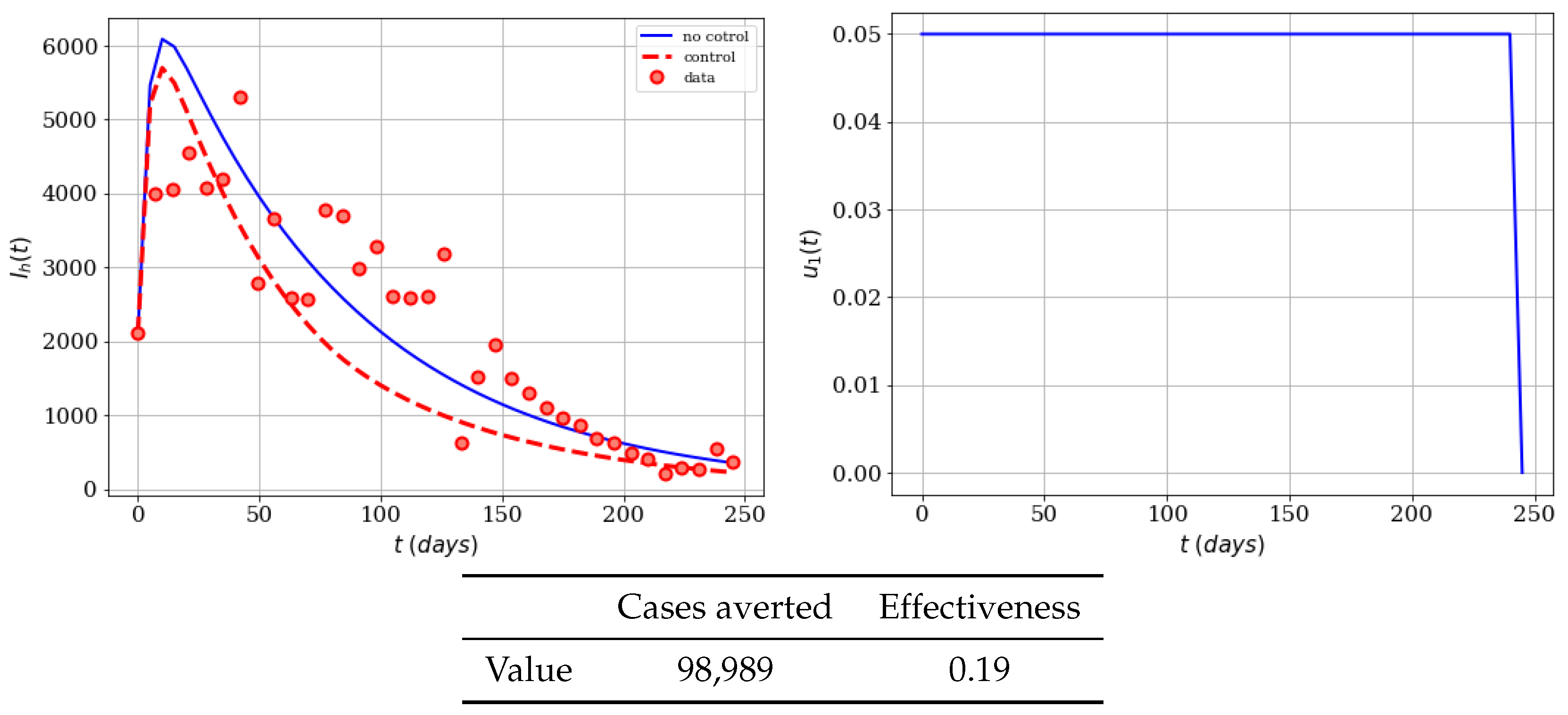
4.1. Mass Educational Campaigns Effects

In this scenario, we consider the case where only the educational campaign policies are implemented as a control policy to minimize the spread of the Zika virus. As we have mentioned before, depending on the viewpoint, we might want to use a different functional $\mathcal{J}$ (4), or even different weights. Several ways can be used to assign the weights depending on costs of each control policy and the cost to health institutions and society of having infected people. For instance, whether infected people might need to see a doctor or occupy a room in a hospital. Thus, here we use a variety of values for the weights ${\kappa }_i$ in order to explore different impacts. We would like to remark that this is an important contribution related to the optimal control that helps with the analysis of the impact of the weights on the solution. Notice that the minimum of the control problem does not change if all the weights are multiplied by a constant. There are infinitely many options from which to choose these weights, but in the real-world, the weights must be assigned based on the priorities of the health institutions and on the costs associated to having an infected and symptomatic individual. In addition, it is important to take into account the costs of each control policy [35,41,42,43]; for example, the cost of educational campaigns. We will use metrics to measure the impact of each time-dependent control $u_1\left(t\right)$ and $u_2\left(t\right)$. The first metric is the total cases avoided by the control strategy during the full time period T [44]. This metric is computed using the following equation

$$Av=T{I}_h\left(0\right)-{\int }_0^T{I}_h^{*}dt,$$

(16)

where $I_h\left(0\right)$ is the initial number of infected persons and $I_h^{*}$ is the infected individuals corresponding to the optimal solution associated with the optimal controls. The second metric is given by:

$$Eff={\displaystyle \frac{Av}{T{I}_h\left(0\right)}}=1-{\displaystyle \frac{{\int }_0^T{I}_h^{*}dt}{T{I}_h\left(0\right)}}.$$

(17)

This second metric is the effectiveness, which is the proportion of the total of avoided cases as compared to the total possible cases under a no intervention attitude [44]. The efficacy function [44] is defined by

$$Ef\left(t\right)={\displaystyle \frac{I_h\left(0\right)-I_h^{*}\left(t\right)}{I_h\left(0\right)}}=1-{\displaystyle \frac{I_h^{*}\left(t\right)}{I_h\left(0\right)}}.$$

(18)

For this first scenario we choose ${\kappa }_1=0.1$, ${\kappa }_3=0.1N_h$, and ${\kappa }_4=0$. This means that we are only interested in minimizing the infected people, and using repellent, insect bednets, and appropriate clothing to avoid the bite of mosquitoes, i.e., just control $u_1$. We choose this particular set in such a way that the terms in the functional $\mathcal{J}$ have a similar order of magnitude, and therefore the weights have impact on the functional $\mathcal{J}$. The functional is given by

$$\mathcal{J}(I_h,u_1)={\int }_0^T\left({\kappa }_1{I}_h+{\kappa }_3{u}_1^2\right)dt.$$

(19)

In this study, we assume that the maximum potential value for the control $u_1$ related to the educational campaign is $u_{1max}=0.5$. This is a particular value that can be changed in a real situation, and depends on the potential efficacy of the control. Notice that assuming $u_{1max}=1$ would give a potential 100% efficacy of the control $u_1$ and therefore no transmission of the Zika virus would happen. We think that this particular situation would be very optimistic for the real world. Therefore we used a more conservative efficacy of 50% ($u_{1max}=0.5$). In Figure 1, the behavior of the infected population with and without control can be seen. In addition, the time-dependent control function $u_1\left(t\right)$ can be observed. We can also see that the implementation of a mass educational campaign would result in a reduction of the number of the infected population at any time. Notice, therefore, that the control stays at its maximum almost during the whole time period and that the effectiveness is not close to 100% since it cannot avoid all the infected cases. This makes sense since the educational campaign will not reach everybody right away. Furthermore, the maximum value that the control $u_1$ takes on during the simulation period is 0.5. In fact, this really means that the use of repellent, insect bednets, and appropriate clothing is necessary in order to have the optimal strategy to reduce the infected people.

The next variation that we include is to choose that the maximum potential value of the control of $u_1$ is $u_{1max}=0.05$ (efficacy of 5%). We can consider this as the population not being able to effectively grasp the educational campaign, and therefore the control will have less impact on avoiding the mosquito bites. Here we expect to have less effectiveness and averted cases. In Figure 2, the infected population with and without control can be seen. We can see that there is a reduction of the number of infected population, but much less than in the previous case, since the control has a maximum value of $u_{1max}=0.05$. Notice that again the control stays at its maximum almost during the whole time period. This means that the use of repellent, insect bednets, and appropriate clothing is necessary in order to have the optimal strategy to reduce the number of infected persons.

Now we include the scenario where the cost of control $u_1$ is reduced to ${\kappa }_3=0.05N_h$, i.e., half of the previous value. We kept the maximum value of the control of $u_1$ as $u_{1max}=0.05$. Since the cost associated to this control $u_1$ is lower, we expect to have more averted cases and effectiveness. In Figure 3, the infected population with and without control can be seen. Notice that control $u_1$ stays at its maximum almost during the whole time period, and the number of averted cases increased due to lower cost of this control. This situation in the real world means that, if for instance the cost of the educational campaign (TV, radio, internet, use of repellent, insect bednets, and appropriate clothing) is reduced then the optimal strategy will reduce even more the number of infected individuals.

4.2. Insecticide Spraying Campaign

Here, we consider that only the insecticide spraying campaign is implemented as a control policy to minimize the spread of the Zika virus by reducing the mosquito population choosing ${\kappa }_1=0.1$, ${\kappa }_3=0$, and ${\kappa }_4\ne 0$. We will minimize the following functional

$$\mathcal{J}(I_h,u_2)={\int }_0^T\left({\kappa }_1{I}_h+{\kappa }_4{u}_2^2\right)dt.$$

(20)

First we choose ${\kappa }_4=0.1N_h$, which is the same associated cost that we initially chose for the mass education campaign. In Figure 4, the trajectories of the infected population with and without control can be seen. It is clear that the insecticide control strategy produces a reduction of the infected population and show the effectiveness of control $u_2\left(t\right)$. This time-dependent control disappears after around 100 days, since there are no infected mosquitoes at that time. Surprisingly, in this case we get better results as compared to the ones with the mass education control policy since we get more averted cases and furthermore the infected subpopulations disappear. Moreover, the control $u_2\left(t\right)$ never reaches the maximum value ($u_{2max}=0.5$) decreases over time, which means that the optimal strategy is to gradually diminish the use of insecticide over the time period. The decision of which control policy would be better might depend on the costs of the mass education (repellent, insect bednets, and appropriate clothing) and application of insecticide controls. In addition, it would depend on the efficacy of the insecticide. Here we kept it at $u_{2max}=0.5$, but in the real-world situation it may be different.

Now we will consider that the maximum value of the control of $u_2$ is $u_{2max}=0.05$, i.e., we reduce the insecticide killing efficacy on mosquitoes. Surprisingly, in this case there is no change since the weights are the same and in the previous case the maximum optimal value reached by control $u_2$ was 0.05. However, if we reduce the $u_{2max}=0.01$ the total averted cases decreases to 277,523 and the effectiveness to 0.53. In this particular case the time-dependent control $u_2\left(t\right)$ needs to be maintained for a longer time due to the reduction of the spraying efficacy on the killing of the mosquitoes.

The last case that we will consider with only insecticide control is lowering the associated cost of this control. Here we assume that ${\kappa }_4=0.01N_h$ and $u_{2max}=0.5$. In Figure 5, we can see (as we expected) that the insecticide control strategy substantially reduces the infected populations, and shows the effectiveness of control $u_2\left(t\right)$. This time-dependent control disappears after about 60 days, since there are no infected mosquitoes at that time. Therefore, no more insecticide is necessary. In a real world situation we might have an infected person coming from another place and a new Zika outbreak might start. The number of averted cases is 433,156, and the effectiveness reaches a value of 0.83. These effects are understandable since the cost associated to control $u_2\left(t\right)$ has been reduced and, therefore, the resources devoted to the implementation of control policies yield better performance.

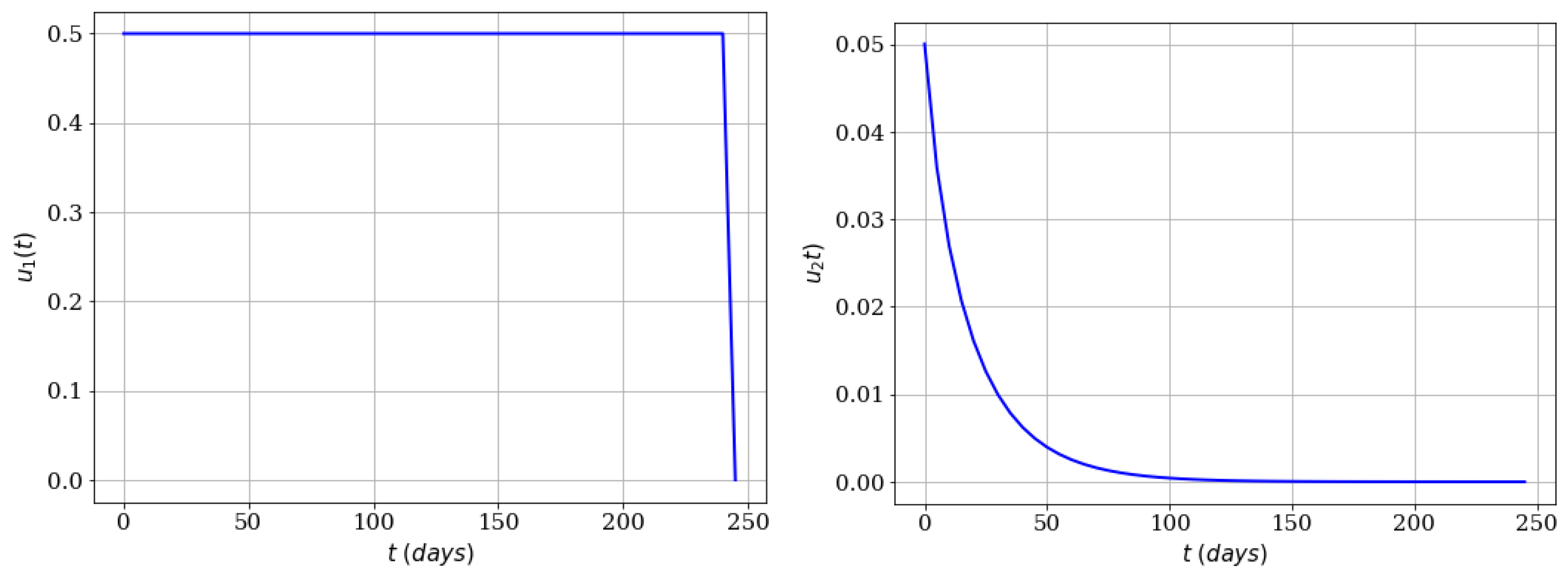
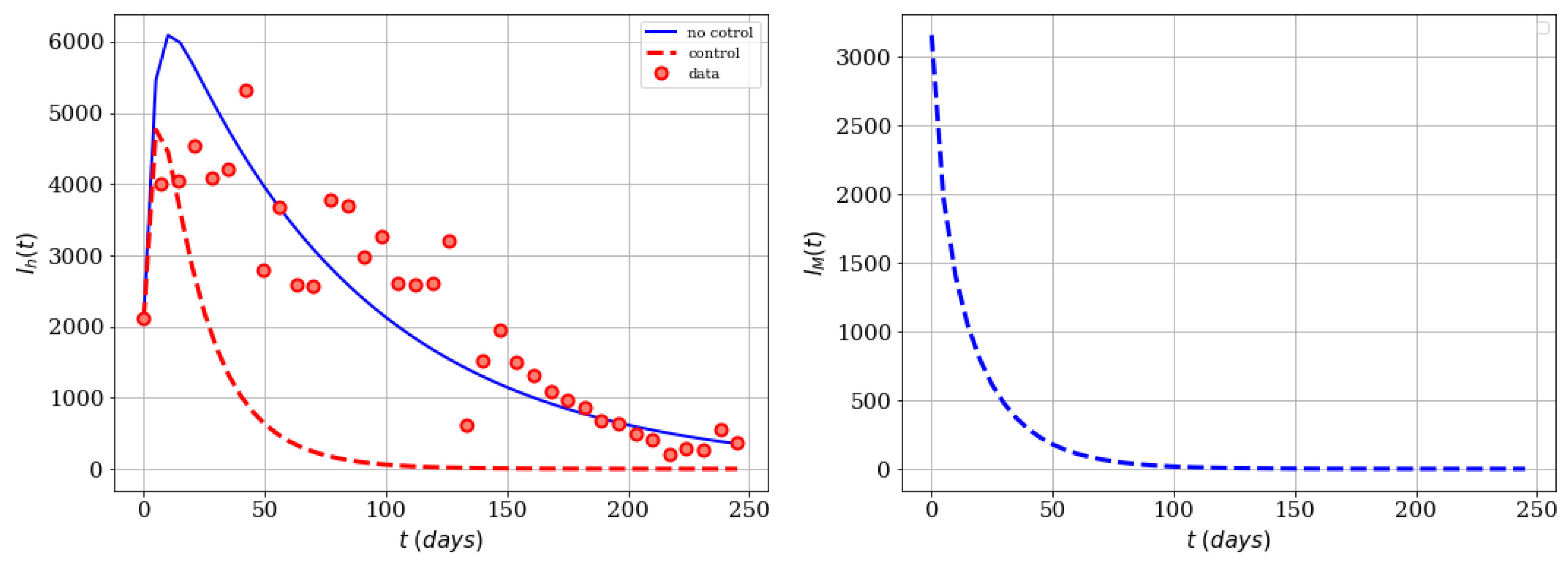
4.3. Mixing the Controls and Including the Infected Mosquitoes

We assume that the cost associated to one infected person is one fold more than the one associated to one infected mosquito. For this scenario we choose ${\kappa }_1=0.1$, ${\kappa }_2=0.01$, and $u_{1max}=u_{2max}=0.5$. This situation means that we want to reduce both infected populations, i.e., $I_h,I_M$. The functional, similar to the one in (4), is given by

$$\mathcal{J}(I_h,I_M,u_1,u_2)={\int }_0^T\left({\kappa }_1{I}_h+{\kappa }_2{I}_M+{\kappa }_3{u}_1^2+{\kappa }_4{u}_2^2\right)dt.$$

(21)

First we only consider mass education control (to use of repellent, insect bednets, and appropriate clothing), i.e., ${\kappa }_4=0$. As can be seen on the left-side of Figure 6, control $u_1$ is used almost during the whole time period in order to reduce the infected population. However, the reduction is lower than in comparison when only the human infected population is included in the functional to be minimized. In fact, the averted cases are 260,096 and the effectiveness is 0.5. Then we did a simulation to consider only an insecticide campaign (${\kappa }_3=0$). Surprisingly, the number of averted cases increased dramatically to 365,464 and the effectiveness to 0.7. Moreover, these results are better than in comparison to when only the human infected population is included in the functional to minimize. On the right-side of Figure 6 it can be seen that control $u_2$ (insecticide) is only necessary for a little bit more than 100 days, and at a maximum optimal value of 0.05. In other words, the time-dependent control related to insecticide seems more efficient to decrease the spread of Zika virus. In this particular case the mosquito population survived, which can be seen as a good outcome from an ecological and biological viewpoint. It is important to remark that here we assume that ${\kappa }_4=0.1N_h$, which is the associated cost related to the insecticide control $u_2$. This value is higher than the one related to infected persons, and that is a factor to explain why the optimal control strategy reduces the insecticide control $u_2$ faster in order to reduce the costs. Nevertheless, in the real world these associated cost values might vary due to different factors.

One last simulation that we would like to present in this subsection is to consider both controls with the same associated cost, i.e., ${\kappa }_3={\kappa }_4$, and with the same amount of resources as in the previous case. Thus, we set ${\kappa }_1=0.09,$ and ${\kappa }_2=0.01$, in a such way that ${\sum }_{i=1}^2{\kappa }_i=0.1$. In regard to the costs of the controls we split resources assigning values ${\kappa }_3={\kappa }_4=0.05N_h$. The simulation of this last scenario, provides an important example of how synergy works for the two controls. Here we obtained better results (same resources) than in comparison with previous cases, where one control was used without the other and vice-versa. The number of averted cases is 384,578 and the effectiveness is 0.74. In Figure 7, it can be seen that both infected populations are reduced and eliminated. Thus, we can conclude that a combination of both controls is the best strategy assuming that the cost associated to one infected person is one fold greater than having one infected mosquito. In the real world, the cost associated to infected people is much higher than the one related to infected mosquitoes. However, we have seen that including the infected mosquito population in the functional is a good strategy to reduce the Zika virus spread.

5. Conclusions and Discussion

We studied and explored the impact that mass educational (to use of repellent, insect bednets, and appropriate clothing) and insecticide campaigns have on the human population risk of infection with the Zika virus. We solved several optimal control problems with different costs associated to the controls and the infected populations, in order to find the best strategies to reduce the spread of the Zika virus in the human population. We relied on Pontryagins’ maximum principle to solve the optimal control problem, which includes a mathematical model for the spread of the Zika virus in human and mosquito populations. To solve the control problem we solved an optimality system, composed by the state system, the adjoint system, initial conditions, transversality conditions, and the optimal controls. We used the indirect method to solve the control problem, which is in nature iterative. We faced some numerical issues that sometimes arise when the indirect method is used. However, adjusting the time step size, we could overcome these numerical issues.

We tackled the optimal problem considering the costs associated to the control campaigns because in the real world this is an essential factor that health institutions and governments consider. We found that the educational campaign (to use of repellent, insect bednets, and appropriate clothing) reduces the number of infected people, but not as well as the insecticide campaign. However, insecticide use can be harmful to the human population and to the environment in general. Therefore, in the real world these factors must be included in the cost associated to the insecticide control. We found that using the same amount of resources it is better to combine or mix both campaigns for more efficient results, regarding the reduction of infected people. We found that there is a synergy effect between the educational (to use of repellent, insect bednets, and appropriate clothing) and insecticide campaigns, and they work better together. We would like to remark that these results assume some particular associated costs for each of the control strategies. However, the approach used here can be extended if different associated costs are used due to real-world aspects. Finally, we found that including the mosquito population in the objective function gives the best results concerning the effectiveness metric that we proposed. We think that this is because one infected human cannot infect another one, and the transmission of Zika virus needs the mosquito vector to spread the Zika virus in the human population.

References

1. Cerbino-Neto, J.; Mesquita, E.C.; Souza, T.M.L.; Parreira, V.; Wittlin, B.B.; Durovni, B.; Lemos, M.C.F.; Vizzoni, A.; de Filippis, A.M.B.; Sampaio, S.A.; et al. Clinical manifestations of Zika virus infection, Rio de Janeiro, Brazil, 2015. Emerg. Infect. Dis. 2016, 22, 1318. [Google Scholar] [CrossRef] [PubMed]
2. González-Parra, G.; Benincasa, T. Mathematical modeling and numerical simulations of Zika in Colombia considering mutation. Math. Comput. Simul. 2019, 163, 1–18. [Google Scholar]
3. Dinh, L.; Chowell, G.; Mizumoto, K.; Nishiura, H. Estimating the subcritical transmissibility of the Zika outbreak in the State of Florida, USA, 2016. Theor. Biol. Med Model. 2016, 13, 20. [Google Scholar] [CrossRef] [PubMed]
4. Tsetsarkin, K.A.; Kenney, H.; Chen, R.; Liu, G.; Manukyan, H.; Whitehead, S.S.; Laassri, M.; Chumakov, K.; Pletnev, A.G. A full-length infectious cDNA clone of Zika virus from the 2015 epidemic in Brazil as a genetic platform for studies of virus-host interactions and vaccine development. mBio 2016, 7, 1–16. [Google Scholar] [CrossRef] [PubMed] [Green Version]
5. Goo, L.; Dowd, K.A.; Smith, A.R.; Pelc, R.S.; DeMaso, C.R.; Pierson, T.C. Zika Virus Is Not Uniquely Stable at Physiological Temperatures Compared to Other Flaviviruses. mBio 2016, 7, 1–16. [Google Scholar] [CrossRef] [PubMed] [Green Version]
6. Hethcote, H.W. Mathematics of infectious diseases. SIAM Rev. 2005, 42, 599–653. [Google Scholar] [CrossRef] [Green Version]
7. Murray, J.D. Mathematical Biology I: An Introduction, Vol. 17 of Interdisciplinary Applied Mathematics; Springer: New York, NY, USA, 2002. [Google Scholar]
8. Diekmann, O.; Heesterbeek, J.; Roberts, M. The construction of next-generation matrices for compartmental epidemic models. J. R. Soc. Interface 2009, 7, 873–885. [Google Scholar] [CrossRef] [Green Version]
9. Khan, M.A.; Iqbal, N.; Khan, Y.; Alzahrani, E. A biological mathematical model of vector-host disease with saturated treatment function and optimal control strategies. Math. Biosci. Eng. 2020, 17, 3972. [Google Scholar] [CrossRef]
10. Khan, M.; Shah, S.W.; Ullah, S.; Gómez-Aguilar, J. A dynamical model of asymptomatic carrier zika virus with optimal control strategies. Nonlinear Anal. Real World Appl. 2019, 50, 144–170. [Google Scholar] [CrossRef]
11. Khan, M.A.; Khan, R.; Khan, Y.; Islam, S. A mathematical analysis of Pine Wilt disease with variable population size and optimal control strategies. Chaos Solitons Fractals 2018, 108, 205–217. [Google Scholar] [CrossRef]
12. Khan, M.; Ali, K.; Bonyah, E.; Okosun, K.; Islam, S.; Khan, A. Mathematical modeling and stability analysis of Pine Wilt Disease with optimal control. Sci. Rep. 2017, 7, 3115. [Google Scholar] [CrossRef]
13. Götz, T.; Altmeier, N.; Bock, W.; Rockenfeller, R.; Wijaya, K.P. Modeling dengue data from Semarang, Indonesia. Ecol. Complex. 2017, 30, 57–62. [Google Scholar] [CrossRef]
14. Bonyah, E.; Khan, M.A.; Okosun, K.; Islam, S. A theoretical model for Zika virus transmission. PLoS ONE 2017, 12, e0185540. [Google Scholar] [CrossRef] [PubMed] [Green Version]
15. Luyten, J.; Beutels, P. The social value of vaccination programs: Beyond cost-effectiveness. Health Aff. 2016, 35, 212–218. [Google Scholar] [CrossRef] [PubMed] [Green Version]
16. Acedo, L.; Diez-Domingo, J.; Morano, J.A.; Villanueva, R.J. Mathematical modelling of respiratory syncytial virus (RSV): Vaccination strategies and budget applications. Epidemiol. Infect. 2010, 138, 853–860. [Google Scholar] [CrossRef]
17. Kumar, A.; Srivastava, P.K. Vaccination and treatment as control interventions in an infectious disease model with their cost optimization. Commun. Nonlinear Sci. Numer. Simul. 2017, 44, 334–343. [Google Scholar] [CrossRef]
18. Kumar, A.; Srivastava, P.K.; Dong, Y.; Takeuchi, Y. Optimal control of infectious disease: Information-induced vaccination and limited treatment. Phys. A Stat. Mech. Appl. 2020, 542, 123196. [Google Scholar] [CrossRef]
19. Barber, L.M.; Schleier, J.J., III; Peterson, R.K. Economic cost analysis of West Nile virus outbreak, Sacramento County, California, USA, 2005. Emerg. Infect. Dis. 2010, 16, 480. [Google Scholar] [CrossRef]
20. Keech, M.; Beardsworth, P. The impact of influenza on working days lost. Pharmacoeconomics 2008, 26, 911–924. [Google Scholar] [CrossRef]
21. Zohrabian, A.; Meltzer, M.I.; Ratard, R.; Billah, K.; Molinari, N.A.; Roy, K.; Scott, R.D. West Nile virus economic impact, Louisiana, 2002. Emerg. Infect. Dis. 2004, 10, 1736. [Google Scholar] [CrossRef]
22. Canali, M.; Rivas-Morales, S.; Beutels, P.; Venturelli, C. The cost of Arbovirus disease prevention in Europe: Area-wide integrated control of tiger mosquito, Aedes albopictus, in Emilia-Romagna, Northern Italy. Int. J. Environ. Res. Public Health 2017, 14, 444. [Google Scholar] [CrossRef]
23. Vanderslice, R.; Porter, N.; Williams, S.; Kulungara, A. Functional Relationship Between Public Health and Mosquito Abatement. In Mosquitoes, Communities, and Public Health in Texas; Elsevier: Amsterdam, The Netherlands, 2020; pp. 359–379. [Google Scholar]
24. Chen-Charpentier, B.M.; Jackson, M. Direct and indirect optimal control applied to plant virus propagation with seasonality and delays. J. Comput. Appl. Math. 2020, 380, 112983. [Google Scholar] [CrossRef]
25. Manore, C.A.; Ostfeld, R.S.; Agusto, F.B.; Gaff, H.; LaDeau, S.L. Defining the risk of Zika and chikungunya virus transmission in human population centers of the eastern United States. PLoS Negl. Trop. Dis. 2017, 11, e0005255. [Google Scholar] [CrossRef]
26. Ghosh, D. Zika virus a global emergency. Curr. Sci. 2018, 114, 725. [Google Scholar]
27. Kakarla, S.G.; Mopuri, R.; Mutheneni, S.R.; Bhimala, K.R.; Kumaraswamy, S.; Kadiri, M.R.; Gouda, K.C.; Upadhyayula, S.M. Temperature dependent transmission potential model for chikungunya in India. Sci. Total. Environ. 2019, 647, 66–74. [Google Scholar] [CrossRef]
28. González-Parra, G.; Dobrovolny, H.M.; Aranda, D.F.; Chen-Charpentier, B.; Rojas, R.A.G. Quantifying rotavirus kinetics in the REH tumor cell line using in vitro data. Virus Res. 2018, 244, 53–63. [Google Scholar] [CrossRef]
29. Raue, A.; Kreutz, C.; Maiwald, T.; Bachmann, J.; Schilling, M.; Klingmüller, U.; Timmer, J. Structural and practical identifiability analysis of partially observed dynamical models by exploiting the profile likelihood. Bioinformatics 2009, 25, 1923–1929. [Google Scholar] [CrossRef] [Green Version]
30. Moulay, D.; Aziz-Alaoui, M.; Kwon, H.D. Optimal control of chikungunya disease: Larvae reduction, treatment and prevention. Math. Biosci. Eng. 2012, 9, 369–392. [Google Scholar]
31. Pontryagin, L.S. Mathematical Theory of Optimal Processes; Routledge: Abingdon-on-Thames, UK, 2018. [Google Scholar]
32. Keller, H.B. Numerical Methods for Two-Point Boundary-Value Problems; Courier Dover Publications: Mineola, NY, USA, 2018. [Google Scholar]
33. Kincaid, D.R.; Cheney, E.W. Numerical Analysis: Mathematics of Scientific Computing; American Mathematical Soc.: Providence, RI, USA, 2002; Volume 2. [Google Scholar]
34. Betts, J.T. Practical Methods for Optimal Control and Estimation Using Nonlinear Programming; SIAM: Philadelphia, PA, USA, 2010; Volume 19. [Google Scholar]
35. Rodrigues, H.S.; Monteiro, M.T.T.; Torres, D.F. Vaccination models and optimal control strategies to dengue. Math. Biosci. 2014, 247, 1–12. [Google Scholar] [CrossRef] [Green Version]
36. Workman, J.T.; Lenhart, S. Optimal Control Applied to Biological Models; Chapman and Hall/CRC: London, UK, 2007. [Google Scholar]
37. Boisvert, J.J.; Muir, P.H.; Spiteri, R.J. py_bvp: A universal Python interface for BVP codes. In Proceedings of the 2010 Spring Simulation Multiconference. Society for Computer Simulation International, Orlando, FL, USA, 11–15 April 2010; p. 95. [Google Scholar]
38. Kierzenka, J.; Shampine, L.F. A BVP solver based on residual control and the Maltab PSE. ACM Trans. Math. Softw. 2001, 27, 299–316. [Google Scholar] [CrossRef]
39. Ascher, U.M.; Mattheij, R.M.; Russell, R.D. Numerical Solution of Boundary Value Problems for Ordinary Differential Equations; SIAM: Philadelphia, PA, USA, 1994; Volume 13. [Google Scholar]
40. Moualeu, D.P.; Weiser, M.; Ehrig, R.; Deuflhard, P. Optimal control for a tuberculosis model with undetected cases in Cameroon. Commun. Nonlinear Sci. Numer. Simul. 2015, 20, 986–1003. [Google Scholar] [CrossRef] [Green Version]
41. Okosun, K.O.; Rachid, O.; Marcus, N. Optimal control strategies and cost-effectiveness analysis of a malaria model. BioSystems 2013, 111, 83–101. [Google Scholar] [CrossRef]
42. Kirschner, D.; Lenhart, S.; Serbin, S. Optimal control of the chemotherapy of HIV. J. Math. Biol. 1997, 35, 775–792. [Google Scholar] [CrossRef] [Green Version]
43. Mohammed-Awel, J.; Agusto, F.; Mickens, R.E.; Gumel, A.B. Mathematical assessment of the role of vector insecticide resistance and feeding/resting behavior on malaria transmission dynamics: Optimal control analysis. Infect. Dis. Model. 2018, 3, 301–321. [Google Scholar] [CrossRef]
44. Rodrigues, P.; Silva, C.J.; Torres, D.F. Cost-effectiveness analysis of optimal control measures for tuberculosis. Bull. Math. Biol. 2014, 76, 2627–2645. [Google Scholar] [CrossRef]
Figure 1. Numerical simulation of an educational campaign ( κ 1 = 0.1 , u 1 m a x = 0.5 ) on the infected humans of the Zika mathematical model (1). Results regarding effectiveness are given in the table. The dots represent the real cases of infected people in Colombia for 2016.
Computation 08 00076 g001
Figure 2. Numerical simulation of an educational campaign ( κ 1 = 0.1 , u 1 m a x = 0.05 ) on the infected humans of the Zika mathematical model (1). Results regarding effectiveness are given in the table. The dots represent the real cases of infected people in Colombia for 2016.
Computation 08 00076 g002
Figure 3. Numerical simulation of an educational campaign ( κ 1 = 0.1 , u 1 m a x = 0.05 ) on the infected humans of the Zika mathematical model (1). Results regarding effectiveness are given in the table. The dots represent the real cases of infected people in Colombia for 2016.
Computation 08 00076 g003
Figure 4. Numerical simulation of insecticide (spraying) campaign ( κ 1 = 0.1 , u 2 m a x = 0.5 ) on the infected humans of the Zika mathematical model (1). Results regarding effectiveness are given in the table. The dots represent the real cases of infected people in Colombia for 2016.
Computation 08 00076 g004
Figure 5. Numerical simulation of insecticide (spraying) campaign ( κ 1 = 0.1 , u 2 m a x = 0.5 ) on the infected humans of the Zika mathematical model (1). Results regarding effectiveness are given in the table. The dots represent the real cases of infected people in Colombia for 2016.
Computation 08 00076 g005
Figure 6. Numerical simulation using both infected subpopulations in the functional ( κ 1 = 0.1 , κ 2 = 0.01 , u 1 m a x = 0.5 ). Left-side with time-dependent control u 1 and right-side just with time-dependent control u 2 .
Computation 08 00076 g006
Figure 7. Numerical simulation using both infected subpopulations in the functional ( κ 1 = 0.09 , κ 2 = 0.01 , u 1 m a x = 0.5 ), and both time-dependent controls u 1 and u 2 .
Computation 08 00076 g007