A High-Order Weakly L-Stable Time Integration Scheme with an Application to Burgers’ Equation

Abstract

In this paper, we propose a 7th order weakly L-stable time integration scheme. In the process of derivation of the scheme, we use explicit backward Taylor’s polynomial approximation of sixth-order and Hermite interpolation polynomial approximation of fifth order. We apply this formula in the vector form in order to solve Burger’s equation, which is a simplified form of Navier-Stokes equation. The literature survey reveals that several methods fail to capture the solutions in the presence of inconsistency and for small values of viscosity, e.g., ${10}^{-3}$, whereas the present scheme produces highly accurate results. To check the effectiveness of the scheme, we examine it over six test problems and generate several tables and figures. All of the calculations are executed with the help of Mathematica 11.3. The stability and convergence of the scheme are also discussed.

1. Introduction

Burgers’ equation with ${\nu }_d$ as coefficient of viscosity can be defined as

$$\frac{\partial \omega }{\partial t}+\omega \frac{\partial \omega }{\partial x}-\frac{{\nu }_d}{2}\frac{{\partial }^2\omega }{\partial x^2}=0,(x,t)\in {\mathsf{\Sigma }}_T,$$

(1)

where

$${\mathsf{\Sigma }}_T=\left({\alpha }_0,{\alpha }_1\right)\times \left(0,T\right],T>0,$$

with boundary conditions (BCs),

$$\omega ({\alpha }_i,t)=0,i=0,1\mathrm{and}t\in (0,T],(\mathrm{Dirichlet} \mathrm{BCs})$$

(2)

and initial condition (IC),

$$\omega (x,0)=f\left(x\right),x\in \left({\alpha }_0,{\alpha }_1\right).$$

(3)

Linearized form of Burgers’ equation (by using Hopf-Cole transformation) is given as

$$\frac{\partial \psi }{\partial t}=\frac{{\nu }_d}{2}\frac{{\partial }^2\psi }{\partial x^2},$$

(4)

with the Neumann boundary conditions (BCs),

$${\psi }_x({\alpha }_i,t)=0,i=0,1,$$

and the initial condition (IC),

$$\psi (x,0)=g\left(x\right).$$

Burgers’ equation is a very simple form of the Navier–Stokes equation and it always attracted researchers due to its occurrence in several areas of physics and applied mathematics, like fluid mechanics, gas dynamics, traffic flow, in the theory of shock waves, and nonlinear acoustics. Firstly, it originated from Bateman [1] in 1915. Later, in 1948, JM Burgers studied it as a class of equation [2,3] to mathematically delineate the turbulence model. Recently, in 2019, Ryu et al. [4] proposed some nowcasting rainfall models that are based on Burger’s equation. Existence and uniqueness of the solution of Equation (1) and its generalized form can be found in [5,6,7].

Recently, due to the availability of high-speed computers, activities that are related to the computation of numerical solution has increased. Özis et al. [8] used finite element approach to solve Burgers’ equation. Dogan [9] proposed a Galerkin finite element method to solve Burgers’ equation. A quadratic and cubic spline collocation method was developed in the paper [10,11,12,13]. Elgindy et al. [14] developed a higher-order numerical scheme by using Hopf-Cole barycentric Gegenbauer integral pseudospectral method. Korkmaz et al. [15] and Jiwari et al. [16] established polynomial based and weighted average based differential quadrature scheme, respectively to solve Burgers’ equation. Verma et al. [17,18] developed Du Fort-Frankel and Douglas finite difference scheme that are unconditionally stable to solve Burgers’ equation. Hassanien et al. [19] developed a two-level three-point finite difference scheme of order 2 in time and order 4 in space to solve Burgers’ equation. Wavelet-based numerical schemes have been developed in [20,21]. Chebyshev collocation method was used in [22,23,24] in order to solve Burgers’ equation, Volterra–Fredholm integral equation, and Riemann-Liouville and Riesz fractional advection-dispersion problems, respectively. Gowrisankar et al. [25] studied singularly perturbed Burgers’ equation.

A well known scheme for diffusion equation is Crank–Nicolson (CN) [26,27,28,29]. CN is a second-order scheme based on Trapezoidal formula which is A-stable but not L-stable. In the presence of inconsistencies [30] or when time step taken is large [27], CN produces unwanted oscillations. As an alternative to CN, Chawla et al. [31] proposed generalized Trapezoidal formula (GTF($\alpha$)) with $\alpha >0$, which is L-stable and gives stable results. Chawla et al. [32] proposed a modified Simpson’s $1/3$ rule (ASIMP), which is A-stable, and used it to give fourth-order time integration formula for diffusion equation, but it suffers from producing unwanted oscillations like CN as it lacks L-stability. To remove these unwanted oscillations, Chawla et al. [33], Lajja et al. [34], and Verma et al. [35] proposed and analyzed various types of L-stable methods, which provides accurate and stable results.

The Burger’s Equation (1) subject to some BCs and IC has an exact solution in the form of Fourier series, which does not converge for small values of viscosity. Hence, it always attracts researchers to test newly developed numerical methods on this nonlinear parabolic PDE.

Here, we derive 7th order time integration formula that is weakly L-stable and generalize the results presented in [33,35]. The issue of slow convergence of series solution for small ${\nu }_d$ forces analytical solution of Equation (1) to diverge from the true solution and, hence, for small values of ${\nu }_d$, it is not easy to compute the solutions. The newly developed method computes the solution even for small ${\nu }_d$. Additionally, it provides satisfactory results in the case of inconsistencies.

We discuss truncation error, stability in detail, in order to show that the developed scheme is convergent. We use software Mathematica 11.3 to compute the solution and Origin $8.5$ for the plotting purpose.

The remainder of this article is constructed, as follows. In Section 2, we give close form solution, which we use to compute the exact solution. In Section 3, we derive a higher-order time integration method for $u^{\prime }\left(t\right)=f(t,u)$. In Section 4, we derive a numerical scheme for the Burgers’ equation. In Section 5, we illustrate the numerical results with tables and two-dimensional (2D)–three-dimensional (3D) graphs.

2. Preliminary

Hopf [36] and Cole [37] suggested that the Equation (1) can be transformed in the form given by

$$\frac{\partial \psi }{\partial t}=\frac{{\nu }_d}{2}\frac{{\partial }^2\psi }{\partial x^2},$$

(5)

with the Neumann BCs

$${\psi }_x({\alpha }_i,t)=0,{\alpha }_i=i,i=0,1,$$

(6)

and the IC

$$\psi (x,0)=g\left(x\right),$$

(7)

by non-linear transformation (Equations (21) and (22), [37])

$$\varphi =-{\nu }_d\left(log\psi \right),\varphi =\varphi (x,t),$$

(8)

and

$$\omega ={\varphi }_x.$$

(9)

Equation (5) can be analytically solved and the solution is given by

$$\psi (x,t)={\beta }_0+\sum _{l=1}^{\infty }{\beta }_{l}exp\left(-\frac{{\nu }_d{l}^2{\pi }^{2}t}{2}\right)cos\left(l\pi x\right),$$

(10)

where ${\beta }_0$ and ${\beta }_l$ are the Fourier coefficients that are given by

$$\begin{array}{ccc}\hfill {\beta }_0& =& {\int }_0^{1}exp\left(-\frac{1}{{\nu }_d}{\int }_0^x{\omega }_0\left(\xi \right)d\xi \right)dx,\hfill \\ \hfill {\beta }_l& =& 2{\int }_0^{1}exp\left(-\frac{1}{{\nu }_d}{\int }_0^x{\omega }_0\left(\xi \right)d\xi \right)cos\left(l\pi x\right)dx,\hfill \end{array}$$

where ${\omega }_0\left(\xi \right)=\omega (\xi ,0)$ and the analytical solution $\omega (x,t)$ of (1) is represented by (Equation (46), [37])

$$\omega (x,t)=\pi {\nu }_d\frac{{\sum }_{l=1}^{\infty }{\beta }_{l}exp(-\frac{{\nu }_d{l}^2{\pi }^{2}t}{2})lsin\left(l\pi x\right)}{{\beta }_0+{\sum }_{l=1}^{\infty }{\beta }_{l}exp(-\frac{{\nu }_d{l}^2{\pi }^{2}t}{2})cos\left(l\pi x\right)}.$$

(11)

3. Illustration of the ProposedMethod

We examine the following initial value problem

$$u^{\prime }\left(t\right)=f(t,u),u\left(t_0\right)={\eta }_0.$$

(12)

The eighth order convergent Newton–Cotes time integration formula is given by

$$u_{n+1}=u_n+\frac{h}{840}\left(41f_n+216f_{n+1/6}+27f_{n+2/6}+272f_{n+3/6}+27f_{n+4/6}+216f_{n+5/6}+41f_{n+1}\right)+\mathcal{O}(h^9).$$

(13)

Now, we use the fifth order Hermite approximation for $u_{n+1/6}$, $u_{n+2/6}$, $u_{n+3/6}$, $u_{n+4/6}$, $u_{n+5/6}$, which are given by

$$\begin{array}{ccc}\hfill u_{n+1/6}& =& \frac{1}{15552}\left(15000u_n+552u_{n+1}+2250h{u}_n^{\prime }-210h{u}_{n+1}^{\prime }+125h^2{u}_n^{″}+25h^2{u}_{n+1}^{″}\right)+\mathcal{O}(h^6),\hfill \end{array}$$

(14)

$$\begin{array}{ccc}\hfill u_{n+2/6}& =& \frac{1}{243}\left(192u_n+51u_{n+1}+48h{u}_n^{\prime }-18h{u}_{n+1}^{\prime }+4h^2{u}_n^{″}+2h^2{u}_{n+1}^{″}\right)+\mathcal{O}(h^6),\hfill \end{array}$$

(15)

$$\begin{array}{ccc}\hfill u_{n+3/6}& =& \frac{1}{64}\left(32u_n+32u_{n+1}+10h{u}_n^{\prime }-10h{u}_{n+1}^{\prime }+h^2{u}_n^{″}+h^2{u}_{n+1}^{″}\right)+\mathcal{O}(h^6),\hfill \end{array}$$

(16)

$$\begin{array}{ccc}\hfill u_{n+4/6}& =& \frac{1}{243}\left(51u_n+192u_{n+1}+18h{u}_n^{\prime }-48h{u}_{n+1}^{\prime }+2h^2{u}_n^{″}+4h^2{u}_{n+1}^{″}\right)+\mathcal{O}(h^6),\hfill \end{array}$$

(17)

$$\begin{array}{ccc}\hfill u_{n+5/6}& =& \frac{1}{15552}\left(552u_n+15000u_{n+1}+210h{u}_n^{\prime }-2250h{u}_{n+1}^{\prime }+25h^2{u}_n^{″}+125h^2{u}_{n+1}^{″}\right)+\mathcal{O}(h^6),\hfill \end{array}$$

(18)

and sixth order Taylor’s approximation

$$\begin{array}{c}{u}_n=u_{n+1}-h{u}_{n+1}^{\prime }+\frac{h^2}{2}{u}_{n+1}^{″}-\frac{h^3}{6}{u}_{n+1}^{‴}+\frac{h^4}{24}{u}_{n+1}^{iv}-\frac{h^5}{120}{u}_{n+1}^v+\mathcal{O}(h^7),\hfill \end{array}$$

(19)

to get

$$\begin{array}{ccc}\hfill \overline{u_{n+1/6}}& =& \frac{1}{46656}[44875u_n+1781u_{n+1}+6750h{u}_n^{\prime }+375h^2{u}_n^{″}-755h{u}_{n+1}^{\prime }+\frac{275}{2}{h}^2{u}_{n+1}^{″}\hfill \\ & & +125(-\frac{h^3}{6}{u}_{n+1}^{‴}+\frac{h^4}{24}{u}_{n+1}^{iv}-\frac{h^5}{120}{u}_{n+1}^v)]+\mathcal{O}(h^6),\hfill \end{array}$$

(20)

$$\begin{array}{ccc}\hfill \overline{u_{n+2/6}}& =& \frac{1}{729}[568u_n+161u_{n+1}+144h{u}_n^{\prime }+12h^2{u}_n^{″}-62h{u}_{n+1}^{\prime }+10h^2{u}_{n+1}^{″}+\hfill \\ & & 8(-\frac{h^3}{6}{u}_{n+1}^{‴}+\frac{h^4}{24}{u}_{n+1}^{iv}-\frac{h^5}{120}{u}_{n+1}^v)]+\mathcal{O}(h^6),\hfill \end{array}$$

(21)

$$\begin{array}{ccc}\hfill \overline{u_{n+3/6}}& =& \frac{1}{64}[31u_n+33u_{n+1}+10h{u}_n^{\prime }+h^2{u}_n^{″}-11h{u}_{n+1}^{\prime }+\frac{3}{2}{h}^2{u}_{n+1}^{″}\hfill \\ & & +(-\frac{h^3}{6}{u}_{n+1}^{‴}+\frac{h^4}{24}{u}_{n+1}^{iv}-\frac{h^5}{120}{u}_{n+1}^v)]+\mathcal{O}(h^6),\hfill \end{array}$$

(22)

$$\begin{array}{ccc}\hfill \overline{u_{n+4/6}}& =& \frac{1}{729}[145u_n+584u_{n+1}+54h{u}_n^{\prime }+6h^2{u}_n^{″}-152h{u}_{n+1}^{\prime }+20h^2{u}_{n+1}^{″}+\hfill \\ & & 8(-\frac{h^3}{6}{u}_{n+1}^{‴}+\frac{h^4}{24}{u}_{n+1}^{iv}-\frac{h^5}{120}{u}_{n+1}^v)]+\mathcal{O}(h^6),\hfill \end{array}$$

(23)

$$\begin{array}{ccc}\hfill \overline{u_{n+5/6}}& =& \frac{1}{46656}[1531u_n+45125u_{n+1}+630h{u}_n^{\prime }+75h^2{u}_n^{″}-6875h{u}_{n+1}^{\prime }+\frac{875}{2}{h}^2{u}_{n+1}^{″}\hfill \\ & & +125(-\frac{h^3}{6}{u}_{n+1}^{‴}+\frac{h^4}{24}{u}_{n+1}^{iv}-\frac{h^5}{120}{u}_{n+1}^v)]+\mathcal{O}(h^6).\hfill \end{array}$$

(24)

Now, we define

$$\begin{array}{c}\overline{f_{n+1/6}}=f(x_{n+1/6},\overline{u_{n+1/6}}),\hfill \end{array}$$

(25)

$$\begin{array}{c}\overline{f_{n+2/6}}=f(x_{n+2/6},\overline{u_{n+2/6}}),\hfill \end{array}$$

(26)

$$\begin{array}{c}\overline{f_{n+3/6}}=f(x_{n+3/6},\overline{u_{n+3/6}}),\hfill \end{array}$$

(27)

$$\begin{array}{c}\overline{f_{n+4/6}}=f(x_{n+4/6},\overline{u_{n+4/6}}),\hfill \end{array}$$

(28)

$$\begin{array}{c}\overline{f_{n+5/6}}=f(x_{n+5/6},\overline{u_{n+5/6}}).\hfill \end{array}$$

(29)

Hence, the time integral formula (13) for the interval $[t_n,t_{n+1}]$ takes the following form

$$\begin{array}{c}\hfill u_{n+1}=u_n+\frac{h}{840}\left(41f_n+216\overline{f_{n+1/6}}+27\overline{f_{n+2/6}}+272\overline{f_{n+3/6}}+27\overline{f_{n+4/6}}+216\overline{f_{n+5/6}}+41f_{n+1}\right).\end{array}$$

(30)

3.1. Local Trunction Error

By applying Taylor’s series expansion, we have

$$\begin{array}{ccc}\hfill u_{n+1/6}& =& \frac{1}{15552}[15000u_n+552u_{n+1}+2250h{u}_n^{\prime }-210h{u}_{n+1}^{\prime }+125h^2{u}_n^{″}\hfill \\ & & +25h^2{u}_{n+1}^{″}]-\frac{25h^6}{6718464}{u}_n^{vi}-\frac{475h^7}{282175488}{u}_n^{vii}+\mathcal{O}(h^8),\hfill \end{array}$$

(31)

$$\begin{array}{ccc}\hfill u_{n+2/6}& =& \frac{1}{243}\left[192u_n+51u_{n+1}+48h{u}_n^{\prime }-18h{u}_{n+1}^{\prime }+4h^2{u}_n^{″}+2h^2{u}_{n+1}^{″}\right]\hfill \\ & & -\frac{h^6}{65610}{u}_n^{vi}-\frac{h^7}{137781}{u}_n^{vii}+\mathcal{O}(h^8),\hfill \end{array}$$

(32)

$$\begin{array}{ccc}\hfill u_{n+3/6}& =& \frac{1}{64}\left[32u_n+32u_{n+1}+10h{u}_n^{\prime }-10h{u}_{n+1}^{\prime }+h^2{u}_n^{″}+h^2{u}_{n+1}^{″}\right]\hfill \\ & & -\frac{h^6}{46080}{u}_n^{vi}-\frac{h^7}{92160}{u}_n^{vii}+\mathcal{O}(h^8),\hfill \end{array}$$

(33)

$$\begin{array}{ccc}\hfill u_{n+4/6}& =& \frac{1}{243}\left[51u_n+192y_{n+1}+18h{u}_n^{\prime }-48h{u}_{n+1}^{\prime }+2h^2{u}_n^{″}+4h^2{u}_{n+1}^{″})\right]\hfill \\ & & -\frac{h^6}{65610}{u}_n^{vi}-\frac{11h^7}{1377810}{u}_n^{vii}+\mathcal{O}(h^8),\hfill \end{array}$$

(34)

$$\begin{array}{ccc}\hfill u_{n+5/6}& =& \frac{1}{15552}[552u_n+15000u_{n+1}+210h{u}_n^{\prime }-2250h{u}_{n+1}^{\prime }+25h^2{u}_n^{″}\hfill \\ & & +125h^2{u}_{n+1}^{″}]-\frac{25h^6}{6718464}{u}_n^{vi}-\frac{575h^7}{282175488}{u}_n^{vii}+\mathcal{O}(h^8),\hfill \end{array}$$

(35)

$$\begin{array}{ccc}\hfill u_n& =& u_{n+1}-h{u}_{n+1}^{\prime }+\frac{h^2}{2}{u}_{n+1}^{″}-\frac{h^3}{6}{u}_{n+1}^{‴}+\frac{h^4}{24}{u}_{n+1}^{iv}-\frac{h^5}{120}{u}_{n+1}^v-\frac{h^6}{720}{u}_n^{vi}\hfill \\ & & -\frac{h^7}{840}{u}_n^{vii}+\mathcal{O}(h^8),\hfill \end{array}$$

(36)

then it follows that

$$\begin{array}{c}{u}_{n+1/6}=\overline{u_{n+1/6}}+\frac{425h^7}{282175488}{u}_n^{vii}+\mathcal{O}(h^8),\hfill \end{array}$$

(37)

$$\begin{array}{c}{u}_{n+2/6}=\overline{u_{n+2/6}}+\frac{4h^7}{688905}{u}_n^{vii}+\mathcal{O}(h^8),\hfill \end{array}$$

(38)

$$\begin{array}{c}{u}_{n+3/6}=\overline{u_{n+3/6}}+\frac{h^7}{129024}{u}_n^{vii}+\mathcal{O}(h^8),\hfill \end{array}$$

(39)

$$\begin{array}{c}{u}_{n+4/6}=\overline{u_{n+4/6}}+\frac{h^7}{196830}{u}_n^{vii}+O(h^8),\hfill \end{array}$$

(40)

$$\begin{array}{c}{u}_{n+5/6}=\overline{u_{n+5/6}}+\frac{325h^7}{282175488}{u}_n^{vii}+\mathcal{O}(h^8).\hfill \end{array}$$

(41)

Also, we have

$$\begin{array}{c}{u}_{n+1}=u_n+\frac{h}{840}[41f_n+216f_{n+1/6}+27f_{n+2/6}+272f_{n+3/6}+27f_{n+4/6}\hfill \\ \hfill +216f_{n+5/6}+41f_{n+1}]-\frac{h^9{u}^{\left(9\right)}}{1567641600}.\end{array}$$

(42)

From all of the above, we deduce that

$$\begin{array}{ccc}\hfill u_{n+1}& =& u_n+\frac{h}{840}(41f_n+216\overline{f_{n+1/6}}+27\overline{f_{n+2/6}}+272\overline{f_{n+3/6}}+27\overline{f_{n+4/6}}\hfill \\ & & +216\overline{f_{n+5/6}}+41f_{n+1})+t_n\left(h\right),\hfill \end{array}$$

(43)

where

$$t_n\left(h\right)=\mathcal{O}(h^8).$$

Thus, the scheme (30) is seventh order convergent. Accordingly, the order of the proposed method is reduced by one, but it is weakly stable, which is a great advantage.

3.2. Stability of the ProposedFormula

Consider the test problem

$$u^{\prime }\left(t\right)=-\lambda u\left(t\right),\lambda >0,$$

(44)

and assume $s=h\lambda$, then we have

$$u_{n+1}=\mathsf{\Psi }\left(s\right)u_n,$$

(45)

where

$$\mathsf{\Psi }\left(s\right)=\frac{540\left(840-414s+84s^2-7s^3\right)}{453600+230040s+48600s^2+5480s^3+540s^4+135s^5+27s^6}.$$

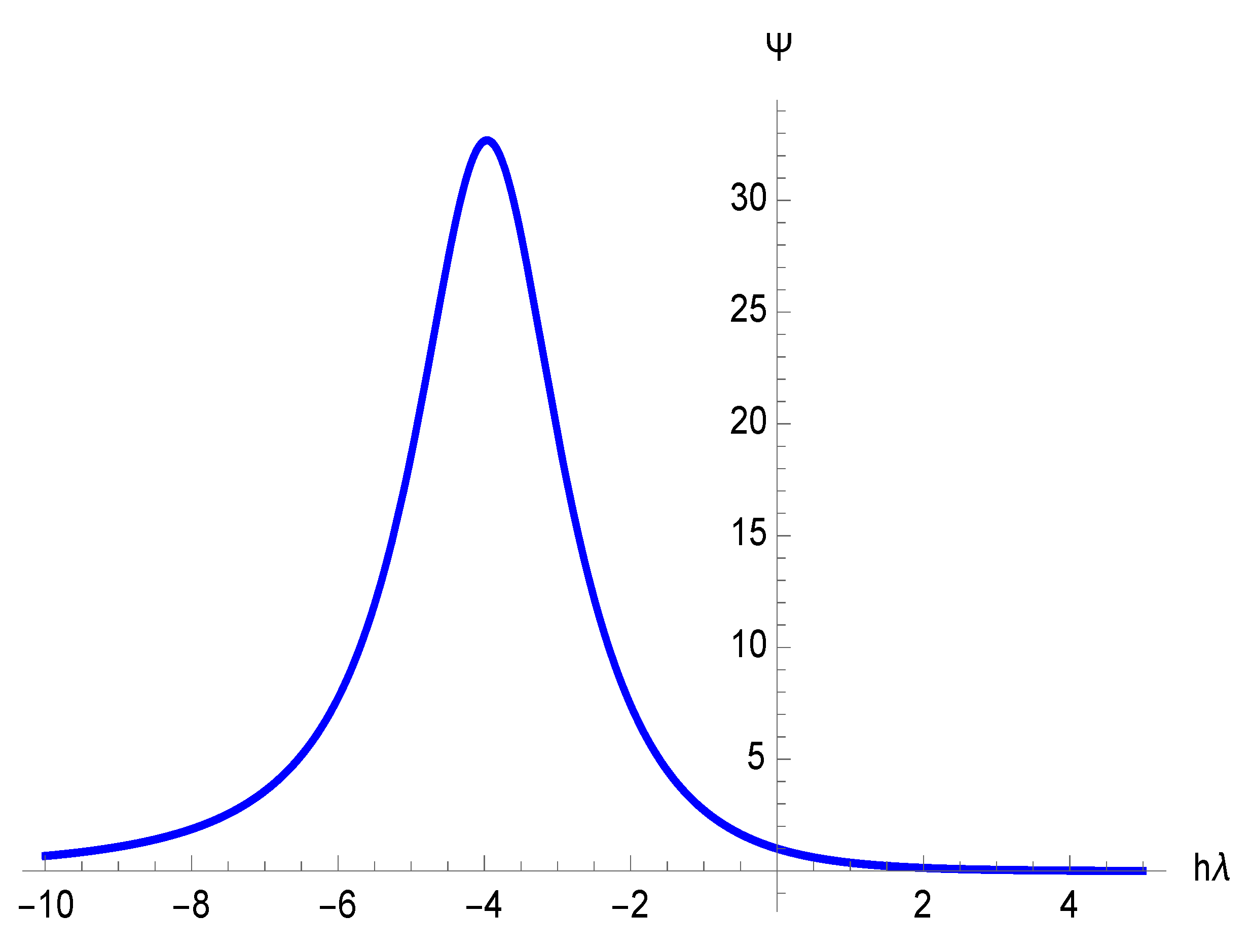
From Figure 1, it can be seen that $\mathsf{\Psi }\left(s\right)\nless 1$ and, hence, our scheme is not A-stable. Since $\mathsf{\Psi }\left(s\right)\to 0$ as $s\to \infty$, the scheme is weakly L-stable (see [35]).

Figure 1. Root of characteristic equation.

3.3. StabilityRegion

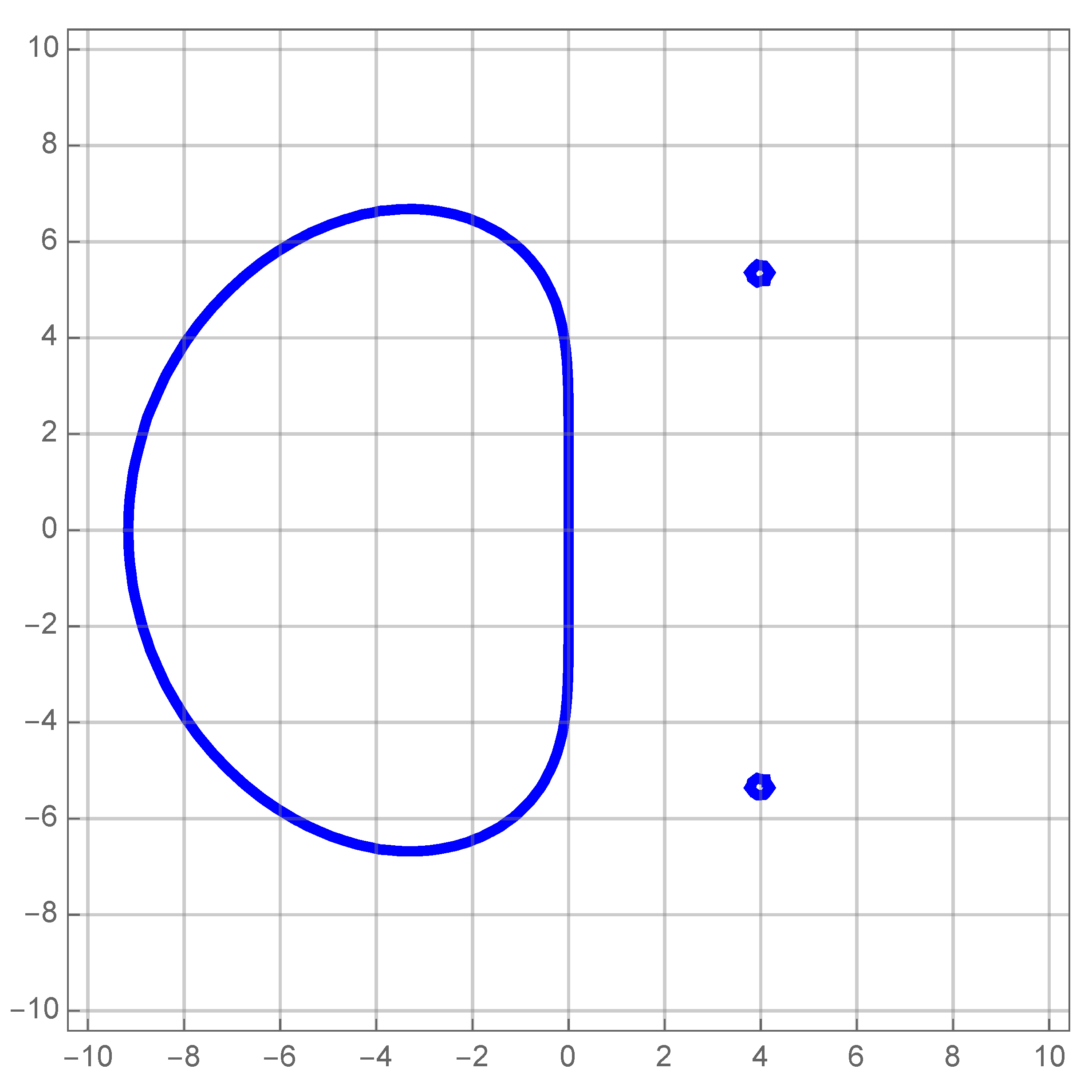
To find the boundary of the stability region, we apply the boundary locus method (p. 64, Chapter 7, [38]). It can be easily seen that, outside of the region (see Figure 2), it is unconditionally stable.

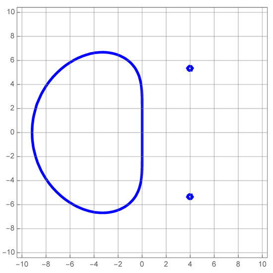
Figure 2. Region of Stability.

4. Application on the Burgers’Equation

4.1. The NumericalScheme

Here, we consider solution space with uniform nodes expressed as ${{\mathsf{\Sigma }}_T}_{i,j}=\{(x_i,t_j):i=0\left(1\right)N,j=0\left(1\right)M\}.$ For that, we partition the interval $\left[{\alpha }_0,{\alpha }_1\right]$ into N (a positive integer) equal sub intervals with the spatial point $x_i=i\Delta x,i=0\left(1\right)N$, where $\Delta x$ is the spatial step.

Additionally, dividing the interval $\left[0,T\right]$ into M equal subintervals with the temporal point $t_j=j\tau ,j=0\left(1\right)M,$ where $\tau =T/M$ and M is a positive integer.

Now, define ${\psi }_i\left(t\right)=\psi (x_i,t)$ and consider Equation (5) and compute the solution $\psi (x_i,t)$ for a given t and for $x_i$ on $\left[{\alpha }_0,{\alpha }_1\right]$. We use (8) and (9) to deduce the following formula for computing the $\omega (x_i,t_j)$

$$\begin{array}{c}\hfill \omega (x_i,t)=\left(\frac{-{\nu }_d}{2\Delta x}\right)\frac{\psi (x_i+\Delta x,t)-\psi (x_i-\Delta x,t)}{\psi (x_i,t)}.\end{array}$$

Now we approximate second order spatial derivative by fourth order central finite difference formula which is given by

$$\begin{array}{c}\hfill \frac{{\partial }^2\psi (x,t)}{{\partial }^{2}x}\approx \frac{16\left(\psi \right(x+\Delta x,t)+\psi (x-\Delta x,t\left)\right)-30\psi (x,t)-\left(\psi \right(x+2\Delta x,t)+\psi (x-2\Delta x,t\left)\right)}{12\Delta x^2},\end{array}$$

and convert the linearized Burgers’ equation into an initial value problem in vector form.

Now, we apply the above finite difference discretization on (5) with the Neumann boundary conditions

$${\psi }_x({\alpha }_i,t)=0,i=0,1,$$

we get the following equation

$$\frac{\partial \mathsf{\Psi }\left(t\right)}{\partial t}=-\frac{{\nu }_d}{24\Delta x^2}D\mathsf{\Psi }\left(t\right),$$

(46)

where $\mathsf{\Psi }\left(t\right)={\left[{\psi }_0\left(t\right),{\psi }_1\left(t\right),{\psi }_2\left(t\right),\dots ,{\psi }_N\left(t\right)\right]}^T$ and D is the $(N+1)\times (N+1)$ pentadiagonal matrix given by

$$D=\left(\begin{array}{cccccccc}30& -32& 2& 0& 0& \cdots & 0& 0\\ -16& 31& -16& 1& 0& \cdots & 0& 0\\ 1& -16& 30& -16& 1& 0& \cdots & 0\\ ⋮& ⋮& \ddots & \ddots & \ddots & \ddots & ⋮& \\ 0& 0& 0& 1& -16& 30& -16& 1\\ 0& 0& 0& 0& 1& -16& 31& -16\\ 0& 0& 0& 0& 0& 2& -32& 30\end{array}\right)$$

(47)

and $\mathsf{\Psi }\left(0\right)=\left[g\left(x_0\right),g\left(x_1\right),g\left(x_2\right),\dots ,g\left(x_N\right)\right].$

Let $\rho ={\nu }_d\tau /24\Delta x^2$, then applying the time integration formula on the initial value problem (46), we obtain

$$\begin{array}{c}{\mathsf{\Psi }}_{j+1}={\mathsf{\Psi }}_j-\frac{\rho }{840}D(41{\mathsf{\Psi }}_j+216\overline{{\mathsf{\Psi }}_{j+1/6}}+27\overline{{\mathsf{\Psi }}_{j+2/6}}+272\overline{{\mathsf{\Psi }}_{j+3/6}}\hfill \\ \hfill +27\overline{{\mathsf{\Psi }}_{j+4/6}}+216\overline{{\mathsf{\Psi }}_{j+5/6}}+41{\mathsf{\Psi }}_{j+1}),\end{array}$$

(48)

where

$$\begin{array}{ccc}\hfill \overline{{\mathsf{\Psi }}_{j+1/6}}& =& \frac{1}{46656}\left[\right(44875I-6750\rho D+375{\rho }^2{D}^2){\mathsf{\Psi }}_j+(1781I+755\rho D\hfill \\ & & +\frac{275}{2}{\rho }^2{D}^2+125(\frac{{\rho }^3{D}^3}{6}+\frac{{\rho }^4{D}^4}{24}+\frac{{\rho }^5{D}^5}{120})\left){\mathsf{\Psi }}_{j+1}\right],\hfill \end{array}$$

(49)

$$\begin{array}{ccc}\hfill \overline{{\mathsf{\Psi }}_{j+2/6}}& =& \frac{1}{729}\left[\right(568I-144\rho D+12{\rho }^2{D}^2){\mathsf{\Psi }}_j+(161I+62\rho D+10{\rho }^2{D}^2\hfill \\ & & +8(\frac{{\rho }^3{D}^3}{6}+\frac{{\rho }^4{D}^4}{24}+\frac{{\rho }^5{D}^5}{120})\left){\mathsf{\Psi }}_{j+1}\right],\hfill \end{array}$$

(50)

$$\begin{array}{ccc}\hfill \overline{{\mathsf{\Psi }}_{j+3/6}}& =& \frac{1}{64}\left[\right(31I-10\rho D+{\rho }^2{D}^2){\mathsf{\Psi }}_j+(33I+11\rho D+\frac{3}{2}{\rho }^2{D}^2+(\frac{{\rho }^3{D}^3}{6}\hfill \\ & & +\frac{{\rho }^4{D}^4}{24}+\frac{{\rho }^5{D}^5}{120})){\mathsf{\Psi }}_{j+1}],\hfill \end{array}$$

(51)

$$\begin{array}{ccc}\hfill \overline{{\mathsf{\Psi }}_{j+4/6}}& =& \frac{1}{729}\left[\right(145I-54\rho D+6{\rho }^2{D}^2){\mathsf{\Psi }}_j+(584I+152\rho D+20{\rho }^2{D}^2\hfill \\ & & +8(\frac{{\rho }^3{D}^3}{6}+\frac{{\rho }^4{D}^4}{24}+\frac{{\rho }^5{D}^5}{120})\left){\mathsf{\Psi }}_{j+1}\right],\hfill \end{array}$$

(52)

$$\begin{array}{ccc}\hfill \overline{{\mathsf{\Psi }}_{j+5/6}}& =& \frac{1}{46656}\left[\right(1531I-630\rho D+75{\rho }^2{D}^2){\mathsf{\Psi }}_j+(45125I+6875\rho D\hfill \\ & & +\frac{875}{2}{\rho }^2{D}^2+125(\frac{{\rho }^3{D}^3}{6}+\frac{{\rho }^4{D}^4}{24}+\frac{{\rho }^5{D}^5}{120})\left){\mathsf{\Psi }}_{j+1}\right].\hfill \end{array}$$

(53)

Now, we use the above defined $\overline{{\mathsf{\Psi }}_{j+1/6}}$, $\overline{{\mathsf{\Psi }}_{j+2/6}}$, $\overline{{\mathsf{\Psi }}_{j+3/6}}$, $\overline{{\mathsf{\Psi }}_{j+4/6}}$, $\overline{{\mathsf{\Psi }}_{j+5/6}}$ in Equation (48) and deduce our final formula used to compute numerical solutions

$$\begin{array}{c}(453600I+2300\rho D+48600{\rho }^2{D}^2+5480{\rho }^3{D}^3+540{\rho }^4{D}^4+135{\rho }^5{D}^5+27{\rho }^6{D}^6)\overline{{\mathsf{\Psi }}_{j+1}}\hfill \\ \hfill =540(840I-414\rho D+84{\rho }^2{D}^2-7{\rho }^3{D}^3)\overline{{\mathsf{\Psi }}_j}.\end{array}$$

(54)

This method is of order $\mathcal{O}(\Delta x^4)+\mathcal{O}\left({\tau }^7\right)$. By using (48), we can compute ${\mathsf{\Psi }}_{j+1}$ and, hence, $w_{ij}$ is computed at different $x_i$’s for a given time level $t_j$. The physical properties of the solutions are discussed later in the form of figures and tables.

4.2. StabilityAnalysis

Equation (48) can be written as

$${\mathsf{\Psi }}_{j+1}=P{\mathsf{\Psi }}_j,$$

where

$$\begin{array}{ccc}\hfill P& =& \frac{540(840I-414\rho D+84{\rho }^2{D}^2-7{\rho }^3{D}^3)}{(453600I+230040\rho D+48600{\rho }^2{D}^2+5480{\rho }^3{D}^3+540{\rho }^4{D}^4+135{\rho }^5{D}^5+27{\rho }^6{D}^6)}\hfill \\ & =& L_1^{-1}{L}_2,\left(\mathrm{say}\right),\hfill \end{array}$$

(55)

where

$$\begin{array}{c}{L}_1=(453600I+230040\rho D+48600{\rho }^2{D}^2+5480{\rho }^3{D}^3+540{\rho }^4{D}^4+135{\rho }^5{D}^5+27{\rho }^6{D}^6)\hfill \\ L_2=540(840I-414\rho D+84{\rho }^2{D}^2-7{\rho }^3{D}^3).\hfill \end{array}$$

Lemma 1.

The matrix P is similar to a symmetric matrix.

Proof. 

Let us introduce a diagonal matrix

$$Q=\left(\begin{array}{ccccc}\sqrt{2}& & & & \\ & 1& & & \\ & & \ddots & & \\ & & & 1& \\ & & & & \sqrt{2}\end{array}\right)$$

such that

$$\tilde{D}=Q^{-1}DQ,$$

i.e., D is similar to a symmetric matrix $\tilde{D}$.

Now, we will show that P is similar to symmetric matrix. Let

$$\begin{array}{c}\hfill \tilde{P}=Q^{-1}PQ=Q^{-1}{L}_1^{-1}{L}_{2}Q=\left[Q^{-1}{L}_1^{-1}Q\right]\left[Q^{-1}{L}_{2}Q\right]\\ \hfill ={\left[Q^{-1}{L}_{1}Q\right]}^{-1}\left[Q^{-1}{L}_{2}Q\right]={\tilde{L}}_1^{-1}{\tilde{L}}_2.\end{array}$$

$$\begin{array}{ccc}\hfill {\tilde{L}}_1& =& (453600I+230040\rho \tilde{D}+48600{\rho }^2{\tilde{D}}^2+5480{\rho }^3{\tilde{D}}^3+540{\rho }^4{\tilde{D}}^4+135{\rho }^5{\tilde{D}}^5+27{\rho }^6{\tilde{D}}^6)\hfill \\ \hfill {\tilde{L}}_2& =& 540(840I-414\rho \tilde{D}+84{\rho }^2{\tilde{D}}^2-7{\rho }^3{\tilde{D}}^3)\hfill \end{array}$$

but matrices ${\tilde{L}}_1^{-1}$ and ${\tilde{L}}_2$ are symmetric and commute and therefore P is similar to a symmetric matrix $\tilde{P}$ and therefore all the eigenvalues of the matrix P are real. □

Lemma 2.

All of the eigenvalues of the matrix D are non-negative.

Proof. 

Let $V=\{v_1,v_2,v_3,\dots ,v_{N+1}\}$ be the eigen vectors of the matrix D corresponding to the eigen value ${\lambda }_l.$ Subsequently, we have

$$\begin{array}{cc}\hfill & (30-{\lambda }_l)v_1-32v_2+2v_3=0,\hfill \end{array}$$

(56)

$$\begin{array}{cc}\hfill & -16v_1+(31-{\lambda }_l)v_2-16v_3+v_4=0,\hfill \end{array}$$

(57)

$$\begin{array}{cc}\hfill & v_{j-2}-16v_{j-1}+(30-{\lambda }_l)v_j-16v_{j+1}+v_{j+2}=0,j=2,3,4,...,N-1,\hfill \end{array}$$

(58)

$$\begin{array}{cc}\hfill & v_{N-2}-16v_{N-1}+(31-{\lambda }_l)v_N-16v_{N+1}=0,\hfill \end{array}$$

(59)

$$\begin{array}{cc}\hfill & 2v_{N-1}-32v_N+(30-{\lambda }_l)v_{N+1}=0.\hfill \end{array}$$

(60)

We set $v_1=v_{-1},v_0=v_2,v_N=v_{N+2},v_{N-1}=v_{N+3}$ then we get fourth order difference equation

$$v_{j-2}-16v_{j-1}+(30-{\lambda }_l)v_j-16v_{j+1}+v_{j+2}=0,j=1,2,\cdots ,N+1,$$

(61)

with the BCs $v_1=v_{-1},v_0=v_2,v_N=v_{N+2},v_{N-1}=v_{N+3}$. The characteristic equation of the Equation (61) is $m^4-16m^3+(30-{\lambda }_l)m^2-16m+1=0$. Assume $m_1,m_2,m_3,m_4$ are the characteristic roots, then we have

$$\begin{array}{c}{m}_1+m_2+m_3+m_4=16,\hfill \\ m_1{m}_2+m_1{m}_3+m_1{m}_4+m_2{m}_3+m_2{m}_4+m_3{m}_4=(30-{\lambda }_l),\hfill \\ m_1{m}_2{m}_3+m_1{m}_3{m}_4+m_2{m}_3{m}_4+m_1{m}_2{m}_4=16,\hfill \\ m_1{m}_2{m}_3{m}_4=1,\hfill \end{array}$$

and the solution is given by $v_j=C_1{m}_1^j+C_2{m}_2^j+C_3{m}_3^j+C_4{m}_4^j$. Let $m_1=r{e}^{i\theta }$ then setting $r=1$, gives ${\lambda }_l=30+2cos2\theta -32cos\theta$. Using Equations (56) and (60) we get $\theta =(2l+1)(\pi /2N),l=0,1,2,\cdots ,N.$ Since V is the non trivial vector satisfying $DV={\lambda }_{l}V$, therefore the eigen values of D are ${\lambda }_l=30+cos((2l+1)\pi /N)-32cos((2l+1)\pi /2N),l=0\left(1\right)N.$ Additionally, it can be shown that ${\lambda }_l\ge 0,\forall l.$ □

Now, let the matrix P has the spectral radius $\varrho \left(P\right)$, then

$$\varrho \left(P\right)=\varrho \left(\overline{P}\right),$$

and it is given by

$$\varrho \left(P\right)\le ma{x}_l\left|{\mu }_l\right|,$$

where ${\mu }_l(l=0,1,2,\cdots ,N)$ are the eigenvalues of the matrix $L_1^{-1}{L}_2$ and therefore

$$\begin{array}{ccc}\hfill {\mu }_l& =& \frac{540(840I-414\rho {\lambda }_l+84{\rho }^2{\lambda }_l^2-7{\rho }^3{\lambda }_l^3)}{(453600I+230040\rho {\lambda }_l+48600{\rho }^2{\lambda }_l^2+5480{\rho }^3{\lambda }_l^3+540{\rho }^4{\lambda }_l^4+135{\rho }^5{\lambda }_l^5+27{\rho }^6{\lambda }_l^6)},\hfill \\ \hfill l=0,1,2,\cdots ,N.& & \end{array}$$

It is clear that the eigen value ${\mu }_l\le 1$ for all possible values of $\rho >0$ and, hence, the method is unconditionally stable. By applying Taylors series expansion, consistency can also be proved easily.

5. NumericalExperiment

To confirm the effectiveness of the proposed weakly L-stable scheme, we apply it to some examples and compute the numerical solutions and depict them in tables and figures. To check the accuracy of the proposed scheme, we also analyze the following type of errors

(i)

Mean root square error norm ($L_2$)

$$\begin{array}{c}\hfill L_2\mathrm{error}=\sqrt{\Delta x\sum _{j=0}^N\mid {\omega }_j^{exact}-{\left({\omega }^{num.}\right)}_j{\mid }^2},\end{array}$$

(62)

and

(ii)

Maximum error norm ($L_{\infty }$)

$$\begin{array}{c}\hfill L_{\infty }\mathrm{error}={\parallel {\omega }^{exact}-{\omega }^{num.}\parallel }_{\infty }=\underset{j}{max}\mid {\omega }_j^{exact}-{\left({\omega }^{num.}\right)}_j\mid ,\end{array}$$

(63)

where ${\omega }^{num.}$ is numerical solution by present method and ${\omega }^{exact}$ is the exact solution and j indicates solution at jth grid point.

5.1. Example 1

Consider the Equation (1) with Dirichlet BCs

$$\omega ({\alpha }_i,t)=0,{\alpha }_i=i,i=0,1\mathrm{and}t\in (0,T],$$

(64)

and IC

$$\omega (x,0)=sin\left(\pi x\right),x\in (0,1),$$

(65)

where ${\nu }_d$ is the coefficient of viscosity. Using the transformation

$$\omega (x,t)=\frac{-{\nu }_d{\psi }_x}{\psi },$$

(66)

Equation (1) is transformed into

$${\psi }_t=\frac{{\nu }_d}{2}{\psi }_{xx},x\in (0,1),t>0,$$

(67)

with IC and BCs

$$\begin{array}{c}\psi (x,0)=exp\left(\frac{1}{\pi {\nu }_d}(cos\pi x-1)\right),\hfill \end{array}$$

(68)

$$\begin{array}{c}{\psi }_x({\alpha }_i,t)=0,{\alpha }_i=i,i=0,1\mathrm{and}t>0.\hfill \end{array}$$

(69)

The solution of the above initial boundary value problem is defined by Equation (11), where

$$\begin{array}{c}{\beta }_0={\int }_0^{1}exp\left(\frac{1}{\pi {\nu }_d}(cos\pi x-1)\right)dx,\hfill \end{array}$$

(70)

$$\begin{array}{c}{\beta }_l=2{\int }_0^{1}exp\left(\frac{1}{\pi {\nu }_d}(cos\pi x-1)cosl\pi x\right)dx.\hfill \end{array}$$

(71)

In this example, we depict several tables and figures and list numerical solutions and exact solutions in order to exhibit the correctness of the scheme. Additionally, we have computed the $L_2$ and $L_{\infty }$ error defined by Equations (62) and (63), respectively. In Table 1, we take ${\nu }_d=2$ and time step $\tau =0.0001$ with $\Delta x=0.0125$. It can be noticed that computed solutions are very close to analytical solutions. It can be seen that, at a specified location, the solution decreases when time passes out. Additionally, it can be seen that, at a fixed moment, the numerical solution first increases and then decreases with changing location from 0 to 1. Table 2 comprise the computed solutions and analytical solutions for ${\nu }_d=0.2,\Delta x=0.0125$ and with the time step $\tau =0.0001$.

Table 1. Computed results and analytical results at different T with ${\nu }_d=2$,$\tau =0.0001$ and $\Delta x=0.0125$ for problem Section 5.1.

x	T = 0.001		T = 0.01		T = 0.1
	${\mathbf{\omega }}^{\mathit{exact}}$	${\mathbf{\omega }}^{\mathit{num}.}$	${\mathbf{\omega }}^{\mathit{exact}}$	${\mathbf{\omega }}^{\mathit{num}.}$	${\mathbf{\omega }}^{\mathbf{exact}}$	${\mathbf{\omega }}^{\mathit{num}.}$
1/10	0.305088	0.304976	0.273239	0.273145	0.109538	0.109509
2/10	0.580565	0.580361	0.521564	0.521393	0.209792	0.209737
3/10	0.799621	0.799363	0.721852	0.721630	0.291896	0.291820
4/10	0.940817	0.940545	0.854590	0.854348	0.347924	0.347834
5/10	0.990174	0.989926	0.905713	0.905483	0.371577	0.371482
6/10	0.942609	0.942407	0.868334	0.868137	0.359046	0.358954
7/10	0.802522	0.802375	0.744098	0.743949	0.309905	0.309827
8/10	0.583466	0.583373	0.543821	0.543723	0.227817	0.227760
9/10	0.306881	0.306837	0.286999	0.286951	0.120687	0.120656
$L_{\infty }error$		2.71275 × 10${}^{-4}$		2.413 × 10${}^{-4}$		9.54852 × 10${}^{-5}$
$L_{2}error$		6.41526 × 10${}^{-5}$		5.82562 × 10${}^{-5}$		2.27535 × 10${}^{-5}$

Table 2. Comparison with existing results by present results for $\Delta x=0.0125,{\nu }_d=0.2,\tau =0.0001$ at different value of T for problem Section 5.1.

x	T	FEM [39]	Asai [40]	${\mathbf{\omega }}^{\mathit{num}.}$	${\mathbf{\omega }}^{\mathit{exact}}$
1/4	0.4	0.31215	0.30891	0.3087531	0.30889
	0.6	0.24360	0.24076	0.2406489	0.24074
	0.8	0.19815	0.19570	0.1956120	0.19568
	1	0.16473	0.16259	0.1625168	0.16256
	3	0.02771	0.02722	0.0271953	0.02720
2/4	0.4	0.57293	0.56970	0.5694998	0.56963
	0.6	0.45088	0.44728	0.4470928	0.44721
	0.8	0.36286	0.35932	0.3591441	0.35924
	1	0.29532	0.29200	0.2918410	0.29192
	3	0.04097	0.04023	0.0401946	0.04021
3/4	0.4	0.63038	0.62567	0.6254715	0.62544
	0.6	0.49268	0.48747	0.4871652	0.48721
	0.8	0.37912	0.37415	0.3738557	0.37392
	1	0.29204	0.28766	0.2874128	0.28747
	3	0.03038	0.02979	0.0297645	0.02977

In Table 2, we can see that the results provided by the present scheme are better than the results in [39]. Additionally, our results are actually better than those of [40]. Table 3 represents that the current scheme gives satisfactory results for viscous coefficient ${\nu }_d=0.01$ with $\Delta x=0.0125$ and $\tau =0.01$ at different times T.

Table 3. Analytical results and numerical results by present method with $\tau =0.01,$ $\Delta x=0.0125$ and ${\nu }_d=0.01$ for problem Section 5.1 at different value of T.

x	T	${\mathbf{\omega }}^{\mathit{num}.}$	${\mathbf{\omega }}^{\mathit{exact}}$
1/4	5	0.046922	0.046963
	10	0.024202	0.024217
	15	0.016300	0.016308
	20	0.012236	0.012240
2/4	5	0.093998	0.093920
	10	0.048414	0.048421
	15	0.032431	0.032439
	20	0.023883	0.023889
3/4	5	0.141354	0.140832
	10	0.071175	0.071134
	15	0.044135	0.044133
	20	0.029155	0.029159

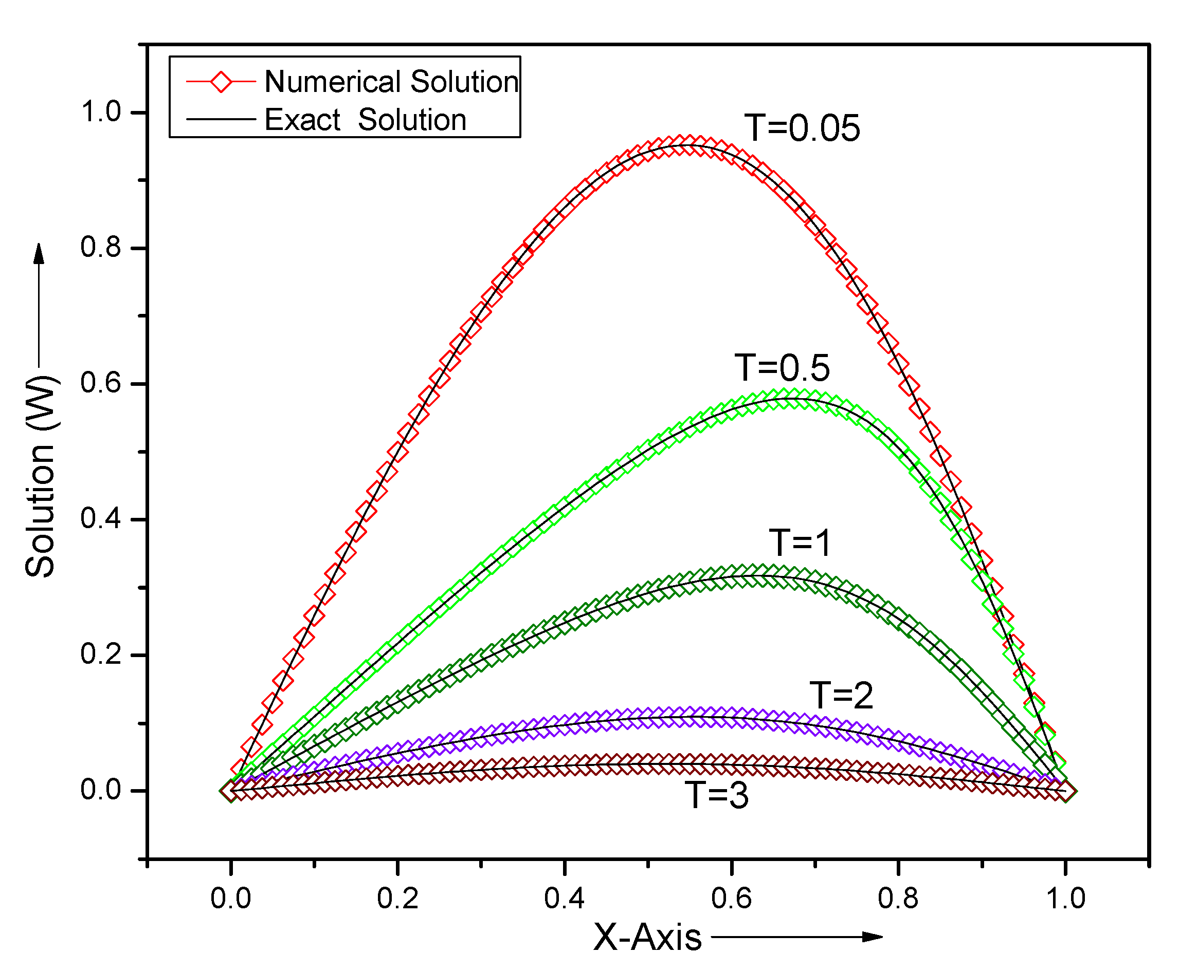
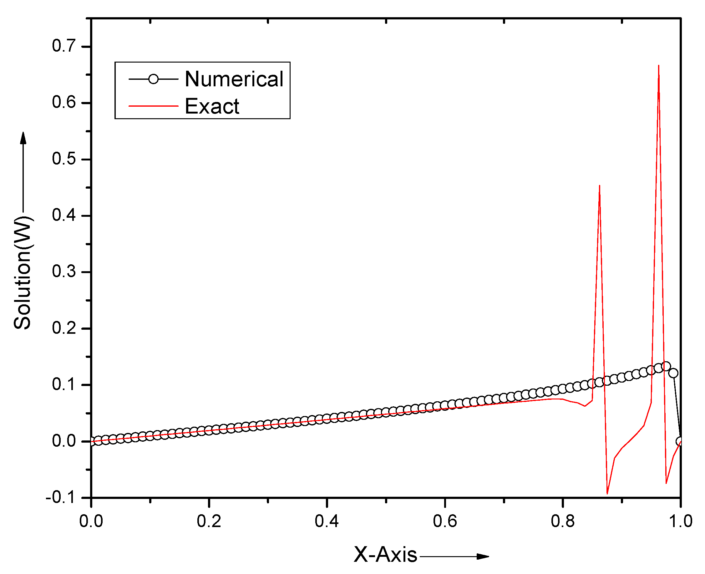
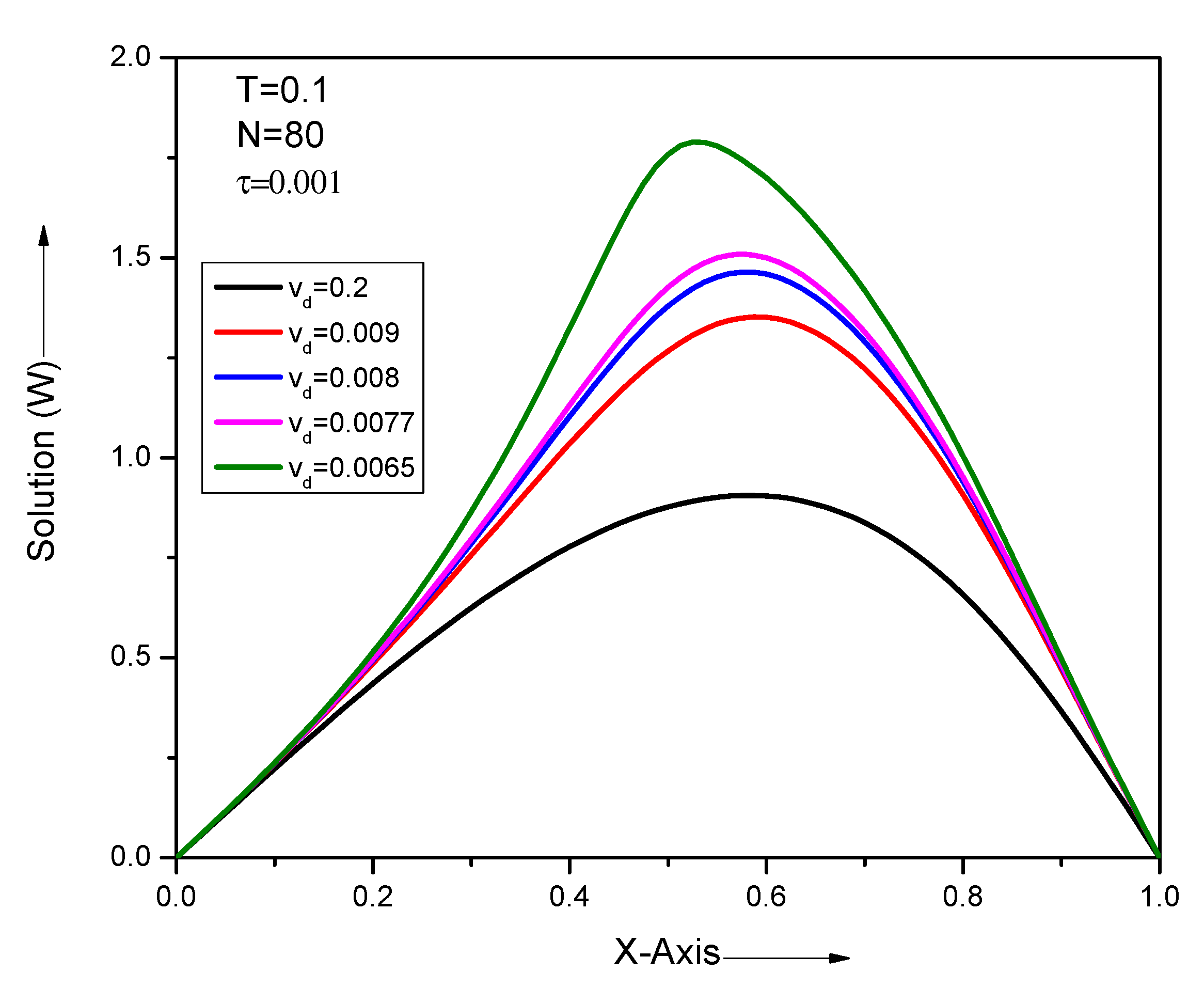
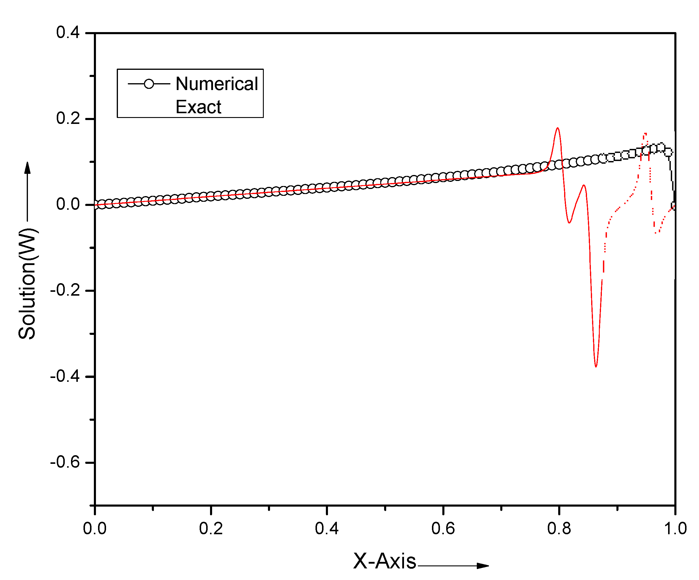
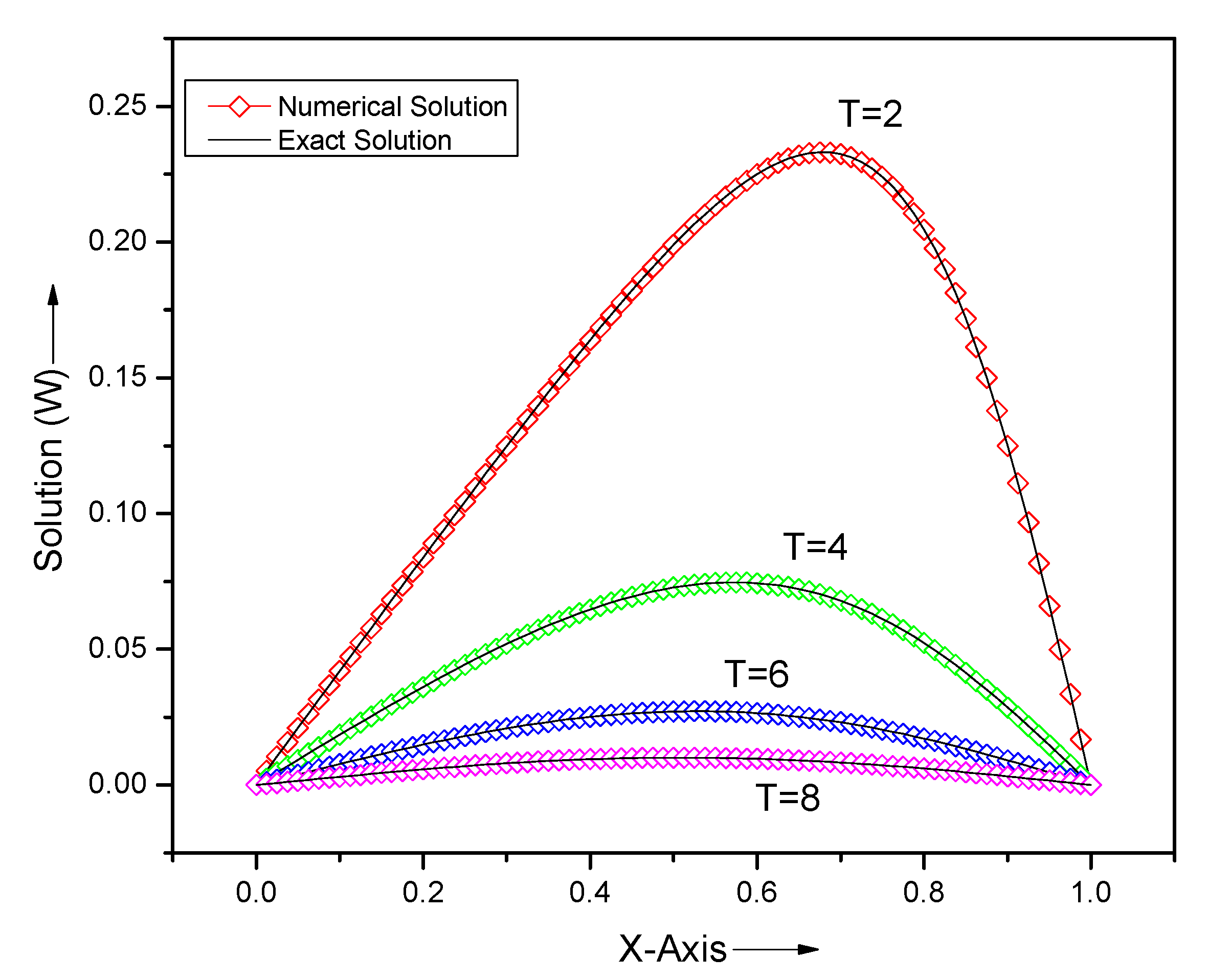
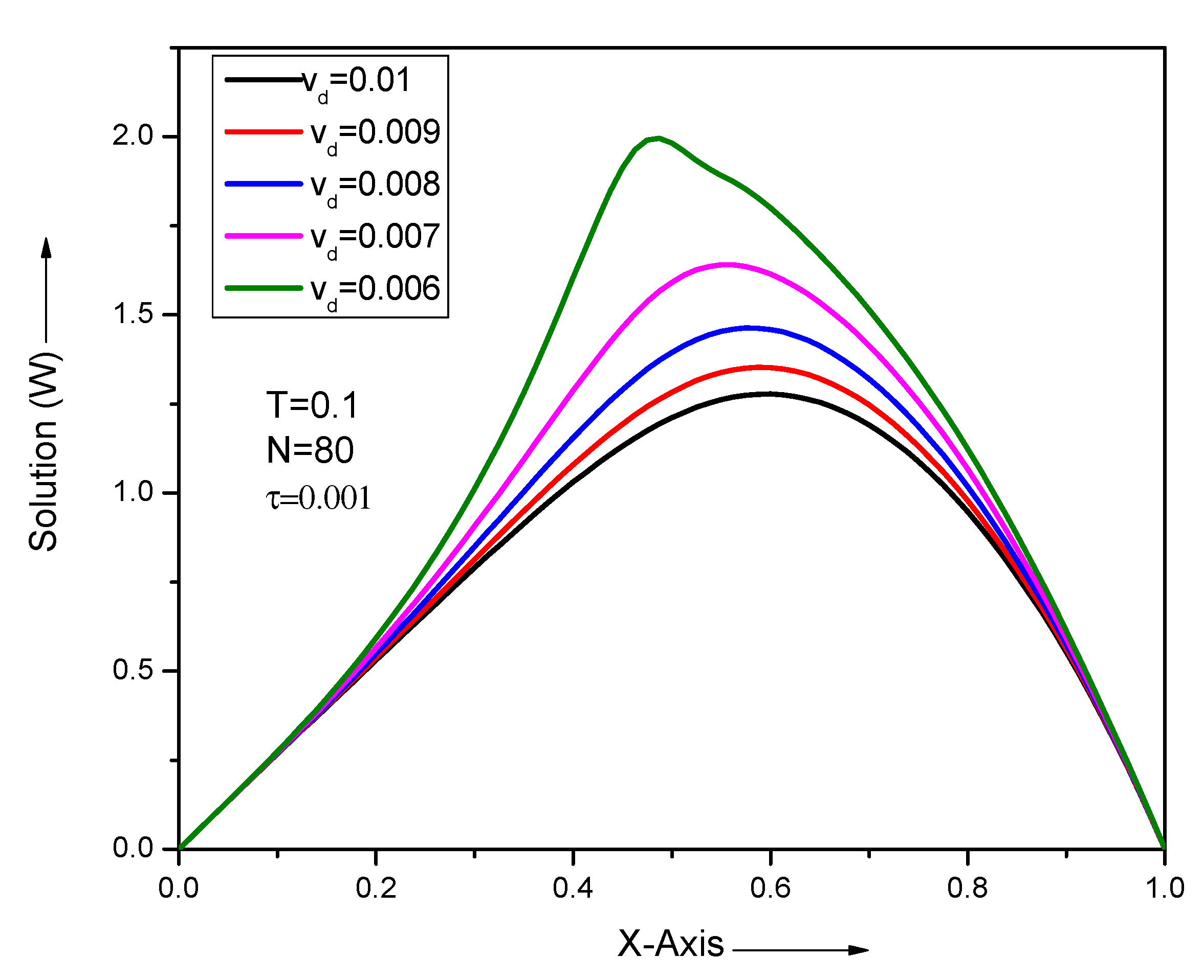
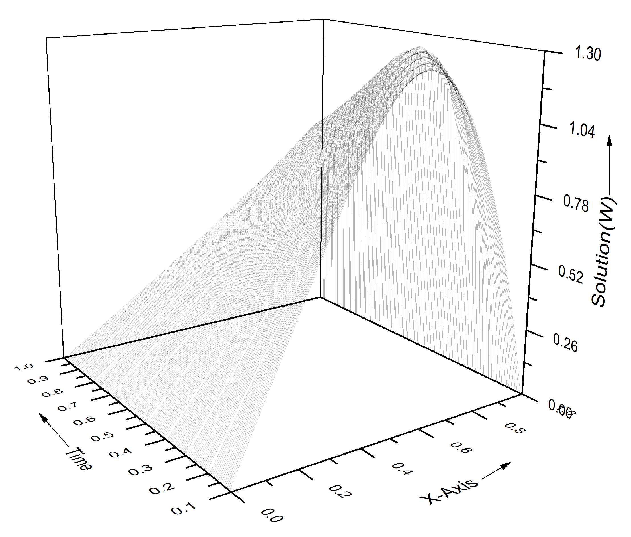
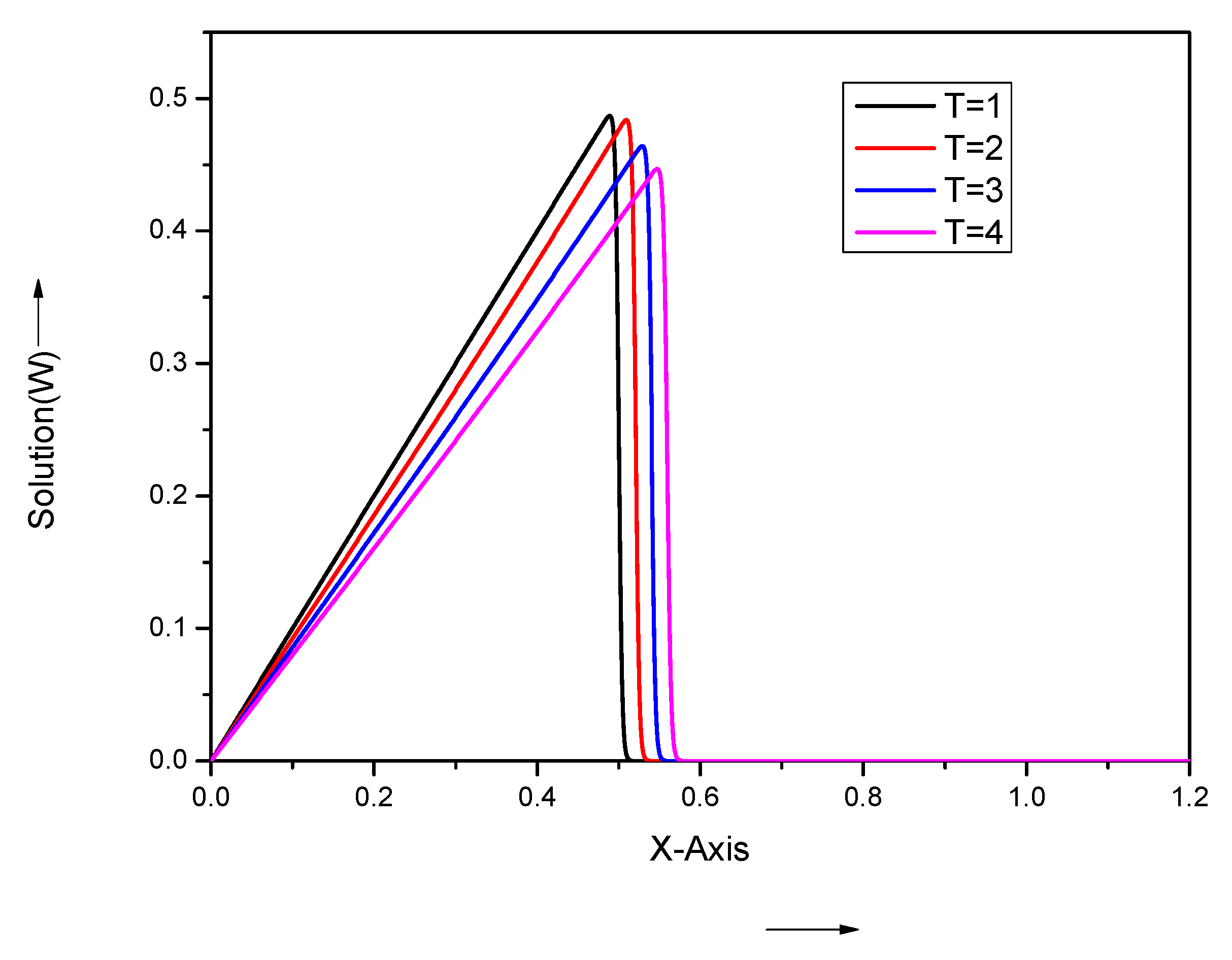
Figure 3 illustrates the accuracy of the present scheme at different times for ${\nu }_d=0.2$ and we are not able to distinguish between the analytical solutions and computed solutions. It is known that the Fourier series solution fails to converge for ${\nu }_d<0.01$ due to the slow convergence rate of infinite series (11). In Figure 4, the analytical solution shows high oscillation, while the computed solutions follow physical behavior. Figure 5 represents the physical behavior of the computed solutions for the different small values of ${\nu }_d$. In Figure 6, we illustrate the physical behavior of the computed results for a small value of ${\nu }_d$ in the three-dimensional mode.

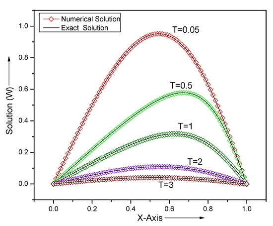
Figure 3. Comparison of analytical and numerical results for problem Section 5.1 with ${\nu }_d=0.2$, $\Delta x=0.0125$ and $\tau =0.001$ and at different times T.

Figure 4. Comparison of analytical and numerical results for problem Section 5.1 at time $T=10$, ${\nu }_d=0.001,\tau =0.001$ and $\Delta x=0.0125$.

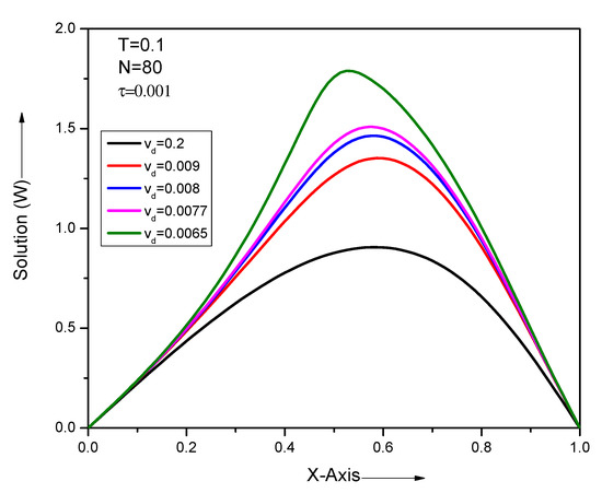
Figure 5. Numerical results for different small values of ${\nu }_d$ with $\tau =0.001$ and $\Delta x=0.0125$ of problem Section 5.1 at time $T=0.1$.

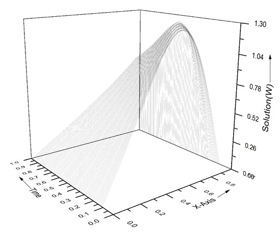
Figure 6. Numerical results with ${\nu }_d=0.01$, $\Delta x=0.0125$ and $\tau =0.001$ at different times T of problem Section 5.1.

5.2. Example 2

Consider Equation (1) with Dirichlet BCs

$$\omega ({\alpha }_i,t)=0,{\alpha }_i=i,i=0,1\mathrm{and}t\in (0,T],$$

(72)

and IC

$$\omega (x,0)=4(1-x)x,x\in (0,1),$$

(73)

where ${\nu }_d$ is the viscous coefficient. Using the transformation

$$\omega (x,t)=\frac{-{\nu }_d{\psi }_x}{\psi },$$

(74)

we see that the Equation (11) represents the analytical solution where

$$\begin{array}{c}{\beta }_0={\int }_0^{1}exp\left(-\frac{2x^2}{3{\nu }_d}(3-2x\right)dx,\hfill \\ {\beta }_l=2{\int }_0^{1}exp\left(-\frac{2x^2}{3{\nu }_d}(3-2x)cosl\pi x\right)dx.\hfill \end{array}$$

In Table 4, we depict the numerical results and compare them with exact solutions for $\tau =0.0001$, ${\nu }_d=2$ with $\Delta x=0.0125$. $L_{\infty }$ and $L_2$-error indicate that the difference between the analytical solution and numerical solution is very less. For the comparison purpose, in Table 5, we take ${\nu }_d=0.2,\tau =0.0001$ and $\Delta x=0.0125$ and notice that the results by the present method are slightly more close to the exact solutions than that given in [39,40]. It can be seen that, at a specified location, the solution decreases when time passes out. Additionally, it can be seen that, at a fixed moment, the numerical solution first increases and then decreases with changing location from 0 to 1. In Table 6, we take $\Delta x=0.0125$, $\tau =0.01$, and ${\nu }_d=0.01$. It can be noticed that solutions that are produced by the present method and analytical solutions are very close to each other.

Table 4. Comparison of analytical and numerical results for $\Delta x=0.0125$, ${\nu }_d=2$, and $\tau =0.0001$ at different value T of the problem Section 5.2.

x	T = 0.001		T = 0.01		T = 0.1
	${\mathbf{\omega }}^{\mathit{exact}}$	${\mathbf{\omega }}^{\mathit{num}.}$	${\mathbf{\omega }}^{\mathit{exact}}$	${\mathbf{\omega }}^{\mathit{num}.}$	${\mathbf{\omega }}^{\mathit{exact}}$	${\mathbf{\omega }}^{\mathit{num}.}$
1/10	0.350947	0.350703	0.294953	0.294822	0.112892	0.112863
2/10	0.630504	0.630240	0.553085	0.552873	0.216252	0.216195
3/10	0.830681	0.830425	0.749751	0.749515	0.300966	0.300887
4/10	0.951242	0.951009	0.873459	0.873232	0.358863	0.358770
5/10	0.991996	0.991794	0.919723	0.919518	0.383422	0.383324
6/10	0.952752	0.952578	0.886239	0.886057	0.370658	0.370563
7/10	0.833318	0.833164	0.771464	0.771302	0.320066	0.319985
8/10	0.633500	0.633351	0.576273	0.576138	0.235371	0.235312
9/10	0.353149	0.352988	0.310136	0.310053	0.124718	0.124687
$L_{\infty }error$		2.64275 × 10${}^{-4}$		2.35909 × 10${}^{-4}$		9.85169 × 10${}^{-5}$
$L_{2}error$		6.55334 × 10${}^{-5}$		6.07706 × 10${}^{-5}$		2.46429 × 10${}^{-5}$

Table 5. Comparison of existing and present results for $\Delta x=0.0125,{\nu }_d=0.2,\tau =0.0001$ at different value of T for problem Section 5.2.

x	T	FEM [39]	Asai [40]	${\mathit{\omega }}^{\mathit{num}.}$	${\mathit{\omega }}^{\mathit{exact}}$
1/4	0.4	0.32091	0.31754	0.317374	0.31752
	0.6	0.24910	0.24616	0.246045	0.24614
	0.8	0.20211	0.19958	0.199490	0.19956
	1	0.16782	0.16562	0.165549	0.16560
	3	0.02828	0.02777	0.027752	0.02776
2/4	0.4	0.58788	0.58460	0.584404	0.58458
	0.6	0.46174	0.45805	0.457862	0.45798
	0.8	0.37111	0.36748	0.367304	0.36740
	1	0.30183	0.29843	0.298267	0.29834
	3	0.04185	0.41090	0.041054	0.04107
3/4	0.4	0.65054	0.64586	0.645660	0.64562
	0.6	0.50825	0.50294	0.502629	0.50268
	0.8	0.39068	0.38557	0.385269	0.38534
	1	0.30057	0.29605	0.295794	0.29586
	3	0.03106	0.03046	0.030432	0.03044

Table 6. Exact and numerical results by present method having ${\nu }_d=0.01,\Delta x=0.0125$ and $\tau =0.01$ at different times T for problem Section 5.2.

x	T	${\mathbf{\omega }}^{\mathit{exact}}$	${\mathbf{\omega }}^{\mathit{num}.}$
1/4	5	0.047415	0.047372
	10	0.024336	0.024321
	15	0.016362	0.016355
	20	0.012272	0.012268
2/4	5	0.094814	0.094895
	10	0.048660	0.048653
	15	0.032550	0.032542
	20	0.023957	0.023951
3/4	5	0.142154	0.142693
	10	0.071517	0.071560
	15	0.044328	0.044330
	20	0.029275	0.029271

In Figure 7, we can see that the exact solution starts oscillating between $x=0.8$ to $x=1$ for a small value of ${\nu }_d=0.001$ due to slow rate of convergence of infinite series, but the results obtained by this method follow the parabolic profile. Figure 8 demonstrates the accuracy of the method for ${\nu }_d=0.1$ and it can be seen that the analytical solution and numerical solution are almost the same at different times throughout the domain. Figure 9 shows that the results that are projected by the present scheme follow the nature of the solutions for different small values of ${\nu }_d$. Figure 10 illustrates the physical nature of the solution in three dimensions.

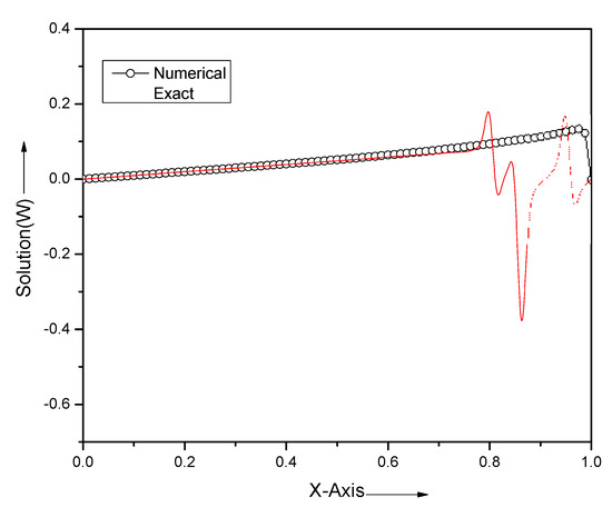
Figure 7. Comparison of analytical and numerical results with ${\nu }_d=0.001$, $\Delta x=0.0125$ and $\tau =0.001$ at time $T=10$ for problem Section 5.2.

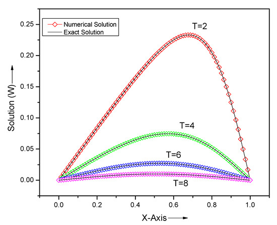
Figure 8. Comparison of analytical and numerical results for problem Section 5.2 at different times T, ${\nu }_d=0.1,\Delta x=0.0125$ and $\tau =0.001$.

Figure 9. Numerical results with different ${\nu }_d$ and $\Delta x=0.0125$, $\tau =0.001$ at time $T=0.1$ for problem Section 5.2.

Figure 10. Three-dimensional (3D) representation of numerical results for problem Section 5.2 for ${\nu }_d=0.01$, $\tau =0.01,\Delta x=0.0125$ and at different times.

5.3. Example 3

Here, we take the exact solution (shock-like) [41] of Equation (1)

$$\omega (x,t)=\frac{\frac{x}{t}}{1+\sqrt{\frac{t}{t_0}{e}^{\frac{x^2}{2{\nu }_{d}t}}}},x\in (0,1.2),t\ge 1,$$

(75)

where $t_0=e^{\frac{1}{4{\nu }_d}}$ having BCs

$$\omega (0,t)=0=\omega (1.2,t),t>1$$

(76)

and IC

$$\omega (x,1)=\frac{x}{1+e^{\frac{1}{2{\nu }_d}(x^2-\frac{1}{4})}},x\in (0,1.2).$$

(77)

In Table 7, for the comparison, we take time step $\tau =0.01$, spatial step $\Delta x=0.0005$ and small value of viscous coefficient ${\nu }_d=0.002$. The numerical solutions at the different discrete points are compared with the existing results presented in [41] and also with the exact solutions. It can be noticed that the results by the present technique are slightly more close to exact solutions than that of given in [41]. For this example, discrete $L_{\infty }$ and $L_2$-error norms are also given and compared with the error that is given in [41]. It can be seen that the error produced by the method in [41] is very high when compared to the error provided by the current scheme. Figure 11 shows the nature of the solutions by present method for small value of ${\nu }_d=0.001$.

Table 7. Comparison of results by present method and existing method and its error for ${\nu }_d=0.002,h=0.0005$ and $\tau =0.01$ at different T for problem Section 5.3.

x	T = 1.7			T = 3.0			T = 3.5
	${\mathbf{\omega }}^{\mathit{exact}}$	${\mathbf{\omega }}^{\mathit{num}.}$	[41]	${\mathbf{\omega }}^{\mathit{exact}}$	${\mathbf{\omega }}^{\mathit{num}.}$	[41]	${\mathbf{\omega }}^{\mathit{exact}}$	${\mathbf{\omega }}^{\mathit{num}.}$	[41]
2/10	0.117647	0.117660	0.11745	0.066667	0.066669	0.06648	0.057143	0.057144	0.05697
4/10	0.235294	0.235420	0.23456	0.133333	0.133355	0.13295	0.114286	0.114299	0.11394
6/10	0.352909	0.353346	0.34936	0.200000	0.200079	0.19922	0.171429	0.171478	0.17082
8/10	0.000000	0.000000	0.00000	0.266618	0.266808	0.26478	0.228571	0.228690	0.22737
${10}^3\times L_{\infty }error$		0.50201	29.70447		0.21289	19.00976		0.16870	16.78871
${10}^3\times L_{2}error$		0.16675	3.59366		0.08135	2.63510		0.06695	2.41729

Figure 11. Numerical results by present method with $\Delta x=0.001$, ${\nu }_d=0.001$ and $\tau =0.01$ at different times T for problem Section 5.3.

5.4. Example 4

We consider the exact solution presented in [42]

$$\begin{array}{c}\hfill \omega (x,t)=\pi {\nu }_d\frac{sin\left(\pi x\right)exp(-{\pi }^2{\nu }_d^{2}t/4)+4sin\left(2\pi x\right)exp(-{\pi }^2{\nu }_d^{2}t)}{4+cos\left(\pi x\right)exp(-{\pi }^2{\nu }_d^{2}t/4)+2cos\left(2\pi x\right)exp(-{\pi }^2{\nu }_d^{2}t)},\end{array}$$

(78)

where initial condition is obtained by putting $t=0$ in (78) and BCs are $\omega (0,t)=0=\omega (2,t)$. The physical behavior of the obtained results by current scheme for ${\nu }_d=0.001,\tau =0.01$ and $\Delta x=0.025$ is exhibited in the Figure 12 left. The absolute errors are presented in Figure 12 right and it is clear that the absolute errors are ≤${10}^{-3}$ for different times. Hence, the numerical results that are obtained by the present method are acceptable.

Figure 12. Numerical approximation (left) and absolute errors (right) of problem Section 5.4 for $\Delta x=0.025,{\nu }_d=0.001,\tau =0.01$ at different times T.

5.5. Example 5

Here, the BCs are same as (2) and IC as

$$\begin{array}{c}\hfill \omega (x,0)=sin\frac{\pi }{2}x,x\in (0,1).\end{array}$$

(79)

Equation (11) represents the analytical solution of the above problem, where

$$\begin{array}{c}{\beta }_0={\int }_0^{1}exp\left(\frac{2}{\pi {\nu }_d}(cos\frac{\pi }{2}x-1)\right)dx,\hfill \end{array}$$

(80)

$$\begin{array}{c}{\beta }_l=2{\int }_0^{1}exp\left(\frac{2}{\pi {\nu }_d}(cos\frac{\pi }{2}x-1)cosl\pi x\right)dx.\hfill \end{array}$$

(81)

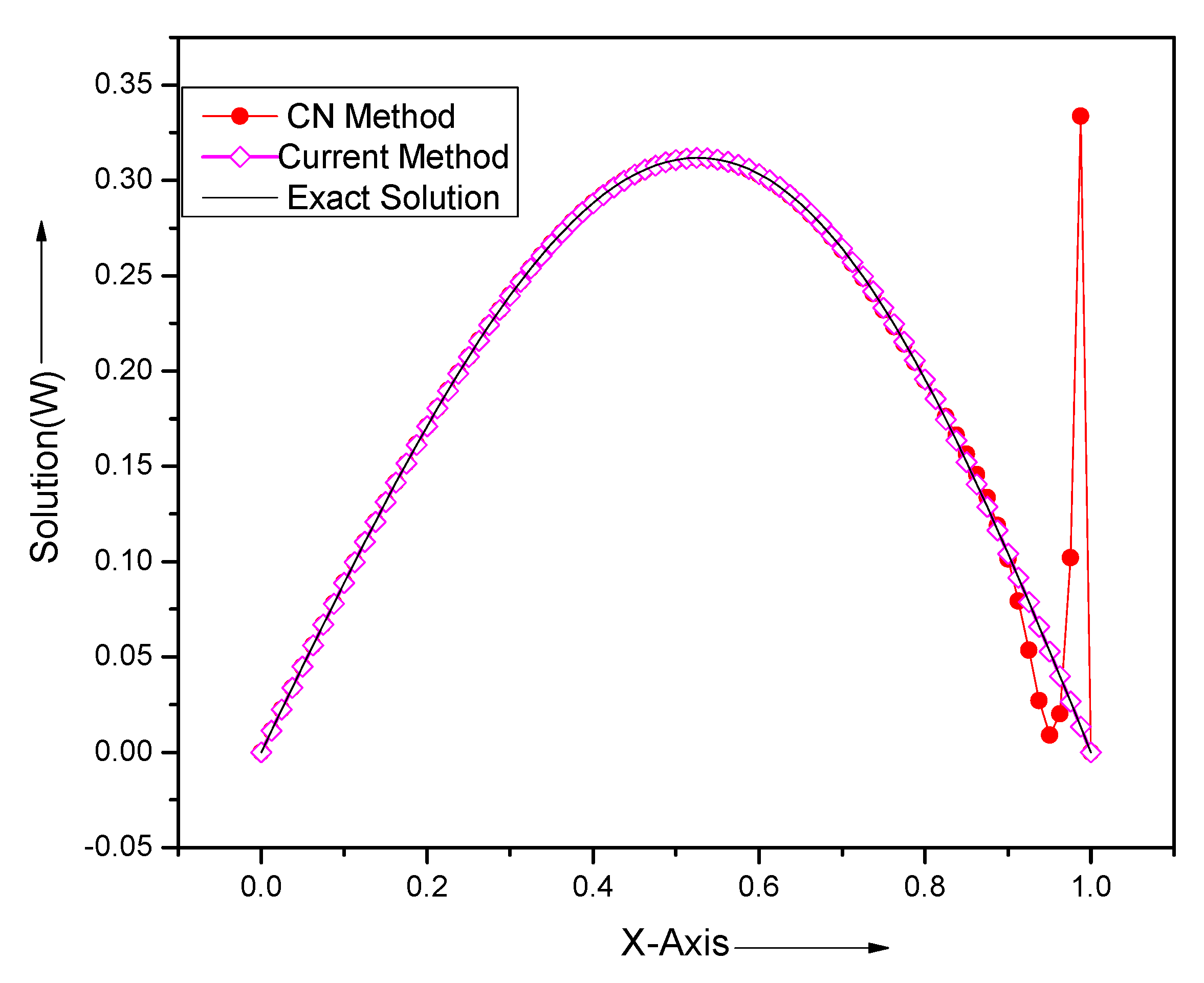
This example shows inconsistent IC and BCs at the boundary point $x=1$. Figure 13 shows high oscillation near the boundary point $x=1$ by the CN method, while the present method gives accurate and stable numerical solutions throughout the domain.

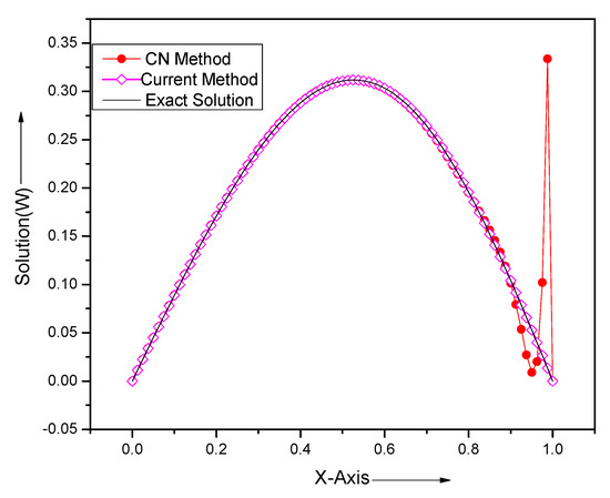
Figure 13. Comparison of analytical solutions and numerical solutions by our method and Crank–Nicolson (CN) method for the problem Section 5.5 at $T=0.1$ for $\Delta x=0.0125,{\nu }_d=2,$ and $\tau =0.01$.

5.6. Example 6

Here, we take the BCs same as (2) and IC as

$$\begin{array}{c}\hfill \omega (x,0)=cos\frac{\pi }{4}x,x\in (0,1).\end{array}$$

(82)

Equation (11) represents the analytical solution of the above problem, where

$$\begin{array}{c}{\beta }_0={\int }_0^{1}exp\left(-\frac{4}{\pi {\nu }_d}sin\frac{\pi }{4}x\right)dx,\hfill \end{array}$$

(83)

$$\begin{array}{c}{\beta }_l=2{\int }_0^{1}exp\left(-\frac{4}{\pi {\nu }_d}\left(sin\frac{\pi }{4}x\right)cosl\pi x\right)dx.\hfill \end{array}$$

(84)

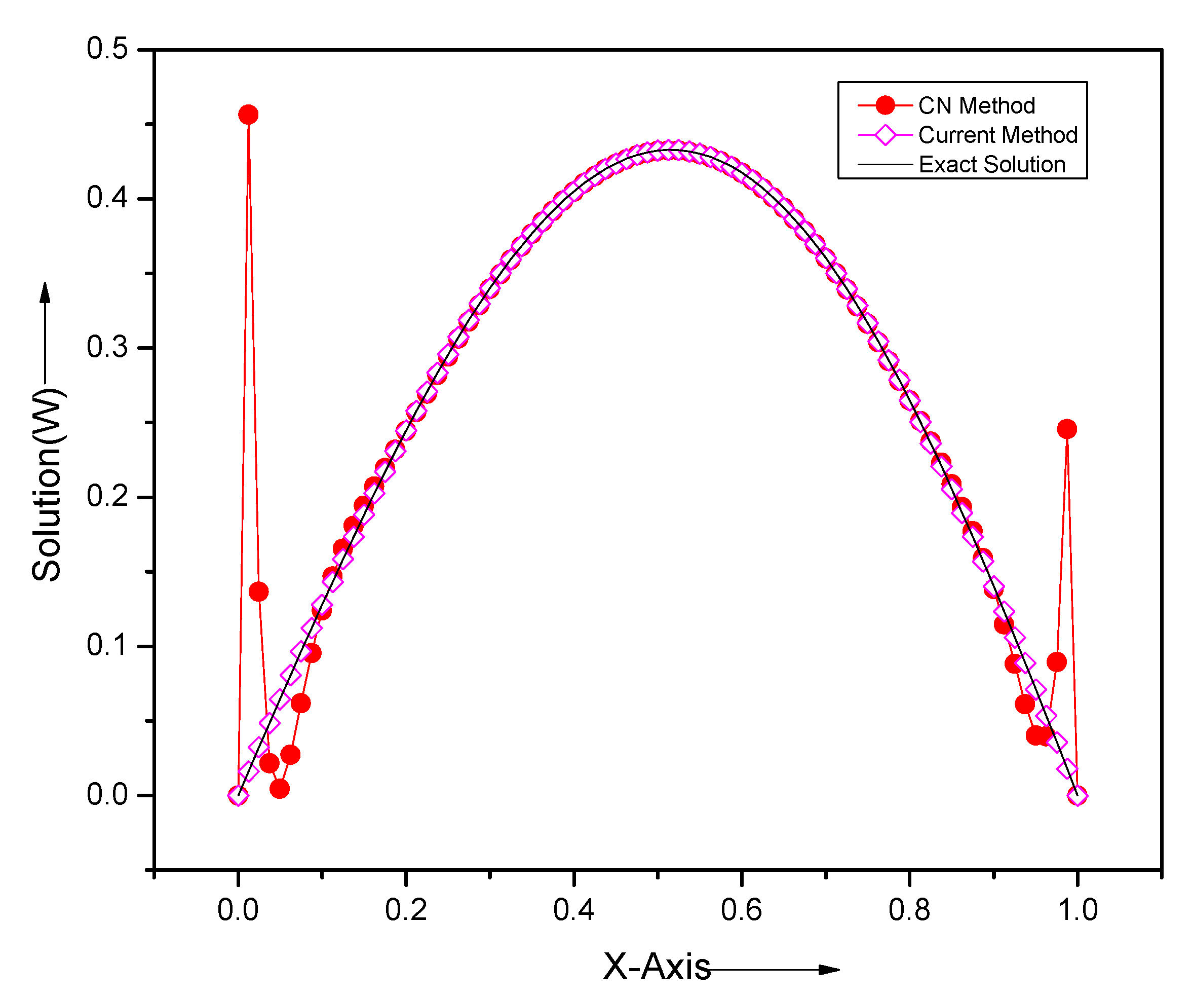
This example shows inconsistent IC and BCs at both the boundary points $x=0$ and $x=1$. From Figure 14, it is clear that the CN method produces high oscillation near both boundary points, while the present method gives accurate and stable numerical solutions throughout the domain.

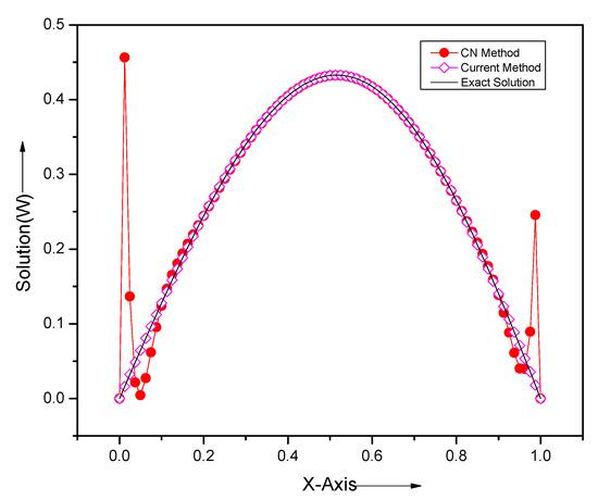
Figure 14. Comparison of analytical solutions and numerical solutions by our method and CN method for the problem Section 5.6 at $T=0.1$ for $\Delta x=0.0125,{\nu }_d=2,$ and $\tau =0.01$.

6. Conclusions

In the present paper, we have used explicit backward Taylor’s series approximation formula of order six and Hermite interpolation polynomial of order five to derive 7th order time integration formula, which is weakly L-stable. The present method is tested over some problems and observed that the approximated results are quite satisfactory and also provides good results when compared to the existing results. It is also observed that the analytical and computed results are very close to each other for small values of viscosity. The strength of this method is that it is easy to apply and takes very little time for computation. It will be interesting to see whether we can give general $n-1$th order convergent weakly L-stable Newton–Cotes formulae by using nth order convergent Newton-Cotes formula. Though the order of the weakly L-stable method is reduced by 1, it is very fruitful for a certain class of nonlinear initial boundary value problems.

References

- Bateman, H. Some recent researches on the motion of fluids. Mon. Weather Rev. 1915, 252, 163–170. [Google Scholar] [CrossRef]
- Burgers, J.M. Mathematical examples illustrating relations occurring in the theory of turbulent fluid motion, Verh. In Selected Papers of JM Burgers; Springer: Dordrecht, The Netherlands, 1939. [Google Scholar]
- Burgers, J.M. A mathematical model illustrating the theory of turbulence. Adv. Appl. Mech. 1948, 1, 171–199. [Google Scholar]
- Ryu, S.; Lyu, G.; Do, Y.; Lee, G.W. Improved rainfall nowcasting using Burgers’ equation. J. Hydrol. 2020, 581, 124140. [Google Scholar] [CrossRef]
- Cecchi, M.M.; Nociforo, R.; Patuzzo, P. Burgers problems-Theoretical results. Riv. Mat. Pura Appl. 1997, 21, 159–174. [Google Scholar]
- Benia, Y.; Sadallah, B.K. Existence of solutions to Burgers equations in domains that can be transformed into rectangles. Electron. J. Differ. Equ. 2016, 2016, 1–13. [Google Scholar]
- Tersenov, A.S. On the generalized Burgers equation. Nonlinear Differ. Equ. Appl. NoDEA 2010, 17, 437–452. [Google Scholar] [CrossRef]
- Öziş, T.; Aksan, E.N.; Özdeş, A. A finite element approach for solution of Burgers’ equation. Appl. Math. Comput. 2003, 139, 417–428. [Google Scholar] [CrossRef]
- Dogan, A. A Galerkin finite element approach to Burgers’ equation. Appl. Math. Comput. 2004, 157, 331–346. [Google Scholar] [CrossRef]
- Aksan, E.N. Quadratic B-spline finite element method for numerical solution of the Burgers’ equation. Appl. Math. Comput. 2006, 174, 884–896. [Google Scholar] [CrossRef]
- Saka, B.; Dağ, I. Quartic B-spline collocation method to the numerical solutions of the Burgers’ equation. Chaos Solitons Fractals 2007, 32, 1125–1137. [Google Scholar] [CrossRef]
- Ali, A.H.A. GA Gardner and LRT Gardner, A collocation solution of Burgers’ equation using cubic B-spline finite element. Comput. Methods Appl. Mech. Eng. 1992, 100, 325–337. [Google Scholar] [CrossRef]
- Korkmaz, A.; Aksoy, A.M.; Dag, I. Quartic B-spline differential quadrature method. Int. J. Nonlinear Sci. 2011, 11, 403–411. [Google Scholar]
- Elgindy, K.T.; Dahy, S.A. High-order numerical solution of viscous Burgers’ equation using a Cole-Hopf barycentric Gegenbauer integral pseudospectral method. Math. Methods Appl. Sci. 2018, 41, 6226–6251. [Google Scholar] [CrossRef]
- Korkmaz, A.; Dag, I. Polynomial based differential quadrature method for numerical solution of nonlinear Burgers’ equation. J. Frankl. Inst. 2011, 348, 2863–2875. [Google Scholar] [CrossRef]
- Jiwari, R.; Mittal, R.C.; Sharma, K.K. A numerical scheme based on weighted average differential quadrature method for the numerical solution of Burgers’ equation. Appl. Math. Comput. 2013, 219, 6680–6691. [Google Scholar]
- Pandey, K.; Verma, L.; Verma, A.K. Du Fort-Frankel finite difference scheme for Burgers equation. Arab. J. Math. 2013, 2, 91–101. [Google Scholar] [CrossRef]
- Pandey, K.; Verma, L.; Verma, A.K. On a finite difference scheme for Burgers’ equation. Appl. Math. Comput. 2009, 215, 2206–2214. [Google Scholar]
- Hassanien, I.A.; Salama, A.A.; Hosham, H.A. Fourth-order finite difference method for solving Burgers’ equation. Appl. Math. Comput. 2005, 150, 781–800. [Google Scholar]
- Jiwari, R. A hybrid numerical scheme for the numerical solution of the Burgers’ equation. Comput. Phys. Commun. 2015, 188, 59–67. [Google Scholar] [CrossRef]
- Shiralashetti, S.C.; Angadi, L.M. Numerical solution of Burgers’ equation using Biorthogonal wavelet-based full approximation scheme. Int. J. Comput. Mater. Sci. Eng. 2019, 8, 1850030. [Google Scholar] [CrossRef]
- Khater, A.H.; Temsah, R.S.; Hassan, M.M. A Chebyshev spectral collocation method for solving Burgers’-type equations. J. Comput. Appl. Math. 2008, 222, 333–350. [Google Scholar] [CrossRef]
- Youssri, Y.H.; Hafez, R.M. Chebyshev collocation treatment of Volterra–Fredholm integral equation with error analysis. Arab. J. Math. 2020, 9, 471–480. [Google Scholar] [CrossRef]
- Doha, E.H.; Abd-Elhameed, W.M.; Elkot, N.A.; Youssri, Y.H. Integral spectral Tchebyshev approach for solving space Riemann-Liouville and Riesz fractional advection-dispersion problems. Adv. Differ. Equ. 2017, 2017, 284. [Google Scholar] [CrossRef][Green Version]
- Gowrisankar, S.; Natesan, S. An efficient robust numerical method for singularly perturbed Burgers’ equation. Appl. Math. Comput. 2019, 346, 385–394. [Google Scholar]
- Crank, J.; Nicolson, P. A practical method for numerical evaluation of solutions of partial differential equations of the heat-conduction type. Adv. Comput. Math. 1947, 6, 207–226. [Google Scholar] [CrossRef]
- Lawson, J.D.; Morris, J.L. The extrapolation of first order methods for parabolic partial differential equations. SIAM J. Numer. Anal. 1978, 15, 1212–1224. [Google Scholar] [CrossRef]
- Smith, G.D. Numerical Solution of Partial Differential Equations: Finite Difference Methods; Oxford University Press: Oxford, UK, 1978. [Google Scholar]
- Thomas, J.W. Numerical Partial Differential Equations: Finite Difference Methods; Springer Science & Business Media: Berlin/Heidelberg, Germany, 2013. [Google Scholar]
- Morton, K.W. Difference Methods for Initial-Value Problems; John Wiley & Sons: Hoboken, NJ, USA, 1967. [Google Scholar]
- Chawla, M.M.; Al-Zanaidi, M.A.; Evans, D.J. Generalized trapezoidal formulas for parabolic equations. Int. J. Comput. Math. 1999, 70, 429–443. [Google Scholar] [CrossRef]
- Chawla, M.M.; Al-Zanaidi, M.A.; Al-Sahhar, M.S. Stabilized fourth order extended methods for the numerical solution of ODEs. Int. J. Comput. Math. 1994, 52, 99–107. [Google Scholar] [CrossRef]
- Chawla, M.M.; Evans, D.J. A new L-stable Simpson-type rule for the diffusion equation. Int. J. Comput. Math. 2005, 82, 601–607. [Google Scholar] [CrossRef]
- Verma, L. L-Stable Derivative-Free Error-Corrected Trapezoidal Rule for Burgers’ Equation with Inconsistent Initial and Boundary Conditions. Int. J. Math. Math. Sci. 2012, 2012, 821907. [Google Scholar] [CrossRef][Green Version]
- Verma, A.K.; Verma, L. Higher order time integration formula with application on Burgers’ equation. Int. J. Comput. Math. 2015, 92, 756–771. [Google Scholar] [CrossRef]
- Hopf, E. The partial differential equation ut + uux = μuxx. Commun. Pure Appl. Math. 1950, 3, 201–230. [Google Scholar] [CrossRef]
- Cole, J.D. On a quasi-linear parabolic equation occurring in aerodynamics. Q. Appl. Math. 1951, 9, 225–236. [Google Scholar] [CrossRef]
- LeVeque, R.J. Finite Difference Methods for Ordinary and Partial Differential Equations; SIAM: Philadelphia, PA, USA, 2007. [Google Scholar]
- Kutluay, S.; Esen, A.; Dag, I. Numerical solutions of the Burgers’ equation by the least-squares quadratic B-spline finite element method. J. Comput. Appl. Math. 2004, 167, 21–33. [Google Scholar] [CrossRef]
- Asaithambi, A. Numerical solution of the Burgers’ equation by automatic differentiation. Appl. Math. Comput. 2010, 216, 2700–2708. [Google Scholar] [CrossRef]
- Xie, S.S.; Heo, S.; Kim, S.; Woo, G.; Yi, S. Numerical solution of one-dimensional Burgers’ equation using reproducing kernel function. J. Comput. Appl. Math. 2008, 214, 417–434. [Google Scholar] [CrossRef]
- Cecchi, M.M.; Nociforo, R.; Grego, P.P. Space-time finite elements numerical solutions of Burgers’ Problems. Matematiche 1996, 51, 43–57. [Google Scholar]
© 2020 by the authors. Licensee MDPI, Basel, Switzerland. This article is an open access article distributed under the terms and conditions of the Creative Commons Attribution (CC BY) license (http://creativecommons.org/licenses/by/4.0/).