A Novel Method for Pressure Mapping between Shell Meshes of Varying Geometries and Resolutions ^†

Abstract

This manuscript discusses a novel method to map pressure results from one 3D surface shell mesh onto another. This method works independently of the actual pressures, and only focuses on ensuring the surface areas consistently match. By utilizing this approach, the cumulative forces consistently match for all input pressures. This method is demonstrated to work for pressure profiles with precipitous changes in pressures, and with small quadrangular source elements being applied to a mix of large quadrangular and triangular target elements, and the forces at all pressure profiles match remarkably.

1. Introduction

Numerical methods [1,2,3,4,5] are among the most important and valuable tools for engineers and scientists today. When an engineering analysis is necessary on an object or domain, and that domain is too complex a shape to be mathematically defined as a simple shape (e.g., a cube, cylinder, or sphere), numerical methods serve to mesh the domain up into clearly defined elements, and the calculating power of a computer can give a realistic answer to the engineering question. One of the most common numerical methods for the study of stresses in a solid is Finite Element Analysis (FEA). Meshed domains are often used in the study of Computational Fluid Dynamics (CFD), an entire field separated from FEA of solids. Of crucial importance in practical engineering is Fluid Solid Interactions (FSI), and, while this is a field in-and-of itself, a combination of CFD and FEA is often used in practical engineering design.

In the studies on the stresses of pressure vessels, water twisters and dynamometers, turbines, airfoils, and countless other applications of fluids and solids, the engineer often uses CFD to model the fluid flow around the incompressible solid, and then uses the pressures at the boundary to study the stresses and strains observed in the solid object. Almost always, the meshed geometry of a CFD domain will vary from the meshed surfaces of an FEA model, and a computational approach to properly map the CFD results onto the FEA boundary is necessary [6,7,8,9,10,11,12,13,14,15,16,17,18,19]. In practical application, it is essential that both the pressure functions match for both meshes, and the cumulative forces in all three dimensions all match for both meshed surfaces. This effort demonstrates a simple and robust algorithm to convert the CFD pressure data into boundary conditions for a different FEA mesh.

There are numerous other efforts to better understand Fluid Solid Interactions (FSI), and interactions between Computational Fluid Dynamics (CFD) and Computational Solid Dynamics (CSD). One such study [20], when using commercial software (ANSYS), approximated a vertical launch tube as a simplified rectangular shape; this was done to validate their novel FSI modeling efforts. Another approach [21] uses the Arbitrary-Lagrangian-Eulerian (ALE) technique, where the shell mesh arbitrarily moves based on pre-determined user assumptions; the algorithm loosely couples the two solvers by applying an arbitrarily specified interface boundary conditions at the beginning of each time step, with specific shell cells to represent the FSI shell border. Remeshing is another approach for unstructured FSI, but it is very computationally expensive [22]. Finally, one of the most common approaches [23,24,25] to map between different shell meshes is to use regression schemes, to develop an equation for the pressure at a given location from a source mesh, and try to match to the target mesh; this approach is realistic, but does not necessarily match the forces perfectly unless one uses very fine meshes.

2. Set-Up

Before a final list of the target pressure data can be produced, a transfer matrix must first be generated. This transfer matrix is data on each target element, which source elements will impact the target pressures, and their weighted averages. Each target element pressure can be defined as the summation of several weighted source pressures

$$\begin{array}{ccc}\hfill P_T& =& {\mathsf{\Sigma }}_{i=1}^N{P}_{S,i}·A_{S,i},\hfill \end{array}$$

(1)

where $P_T$ (Pa) is the target pressure, $P_{S,i}$ is the pressure of N specific sources i, where i is defined by the transfer matrix, and $A_{S,i}$ is the dimensionless weight of each source element’s impact on the target. It is absolutely possible for a source to have an impact on more than one target, although in practice the overwhelming majority of the force from one source will go to one target. The purpose of generating a transfer matrix that is exclusively dependent on the geometry is because, in practice, when one conducts a CFD simulation for FSI, it is often with multiple time-steps and therefore a parametric FEA study will be conducted using a series of pressure data for varying time-steps. With the transfer matrix, one can make sure the cumulative forces in all three directions match consistently regardless of the specific CFD pressure profile.

The first step in this mapping algorithm is to define the element surfaces for both the source mesh and the target. This is comprised of matrices of nodes and elements. The node matrices, both the source and the target, have dimensions of $N_{N,S}·3$ and $N_{N,T}·3$, where $N_{N,S}$ and $N_{N,T}$ represent the number of source and target nodes. These represent the X, Y, and Z coordinates of the nodes, and they are in real or double precision format. There also are two element matrices, of dimensions $N_{E,S}·5$ and $N_{E,T}·5$, where $N_{E,S}$ and $N_{E,T}$ represent the number of source and target elements, and they are in integer format. Each row of these two matrices represents a unique element, which is comprised of the number of nodes in the element (three for linear triangles or four for linear quads; this algorithm does not process quadratic element faces), followed by the integer value for the row in the node matrix that contains the X-Y-Z coordinate for the specific node. If there is a triangle element, the fourth node is listed simply as 0. For example, a quad with coordinates at (1,1,0), (1,2,1), (2,1,0), and (2,2,1) would be listed in the element matrix as

$$\begin{array}{c}\hfill 41234,\end{array}$$

(2)

whereas the first four nodes of the node matrix would be

$$\begin{array}{c}1.01.00.0\hfill \\ 1.02.01.0\hfill \\ 2.01.00.0\hfill \\ 2.02.01.0.\hfill \end{array}$$

(3)

While each element declared will be used in the generation of the transfer matrix, there can be excess nodes in the node matrix without any detriment, so long as all of the nodes referenced by the elements are present.

The next step is to determine the centroid of each element, for linear tetrahedral faces (triangles) and linear hexahedrals faces (quads); this is simply calculated by taking the X, Y, and Z coordinate values of the three or four nodes that comprise the element. Each element row has three columns, regardless of the shape of the element face, for the X, Y, and Z coordinates of the centroid of each element. The centroid is necessary for applying a smoothing function in between elements, which is directly related to the distance between centroids. A separate centroid matrix is assigned for both the source and the target elements, with the dimensions of $N_{E,S}·3$ and $N_{E,T}·3$.

The next step is to calculate the area of each element face. This is performed by taking the cross product of the vectors between the element node and the center of the triangle. If the element is a triangle, it is split into three mini-triangles formed with the vectors from the node to the centroid. The steps are as follows:

• Find the centroid of the triangle element, and in the case of an element being a quad, the triangle that forms half of the quad element surface

  –

  If a quad, then the first three node elements are used to calculate the area. Afterwards, the process is repeated with the first, second, and fourth node. Regardless of the node order, this should create two triangles that form the quad.

  –

  The centroid coordinates are found by simply averaging the X, Y, and Z locations of the three nodes that made up the surface triangle.

• Generate the vectors from each node to the centroid.
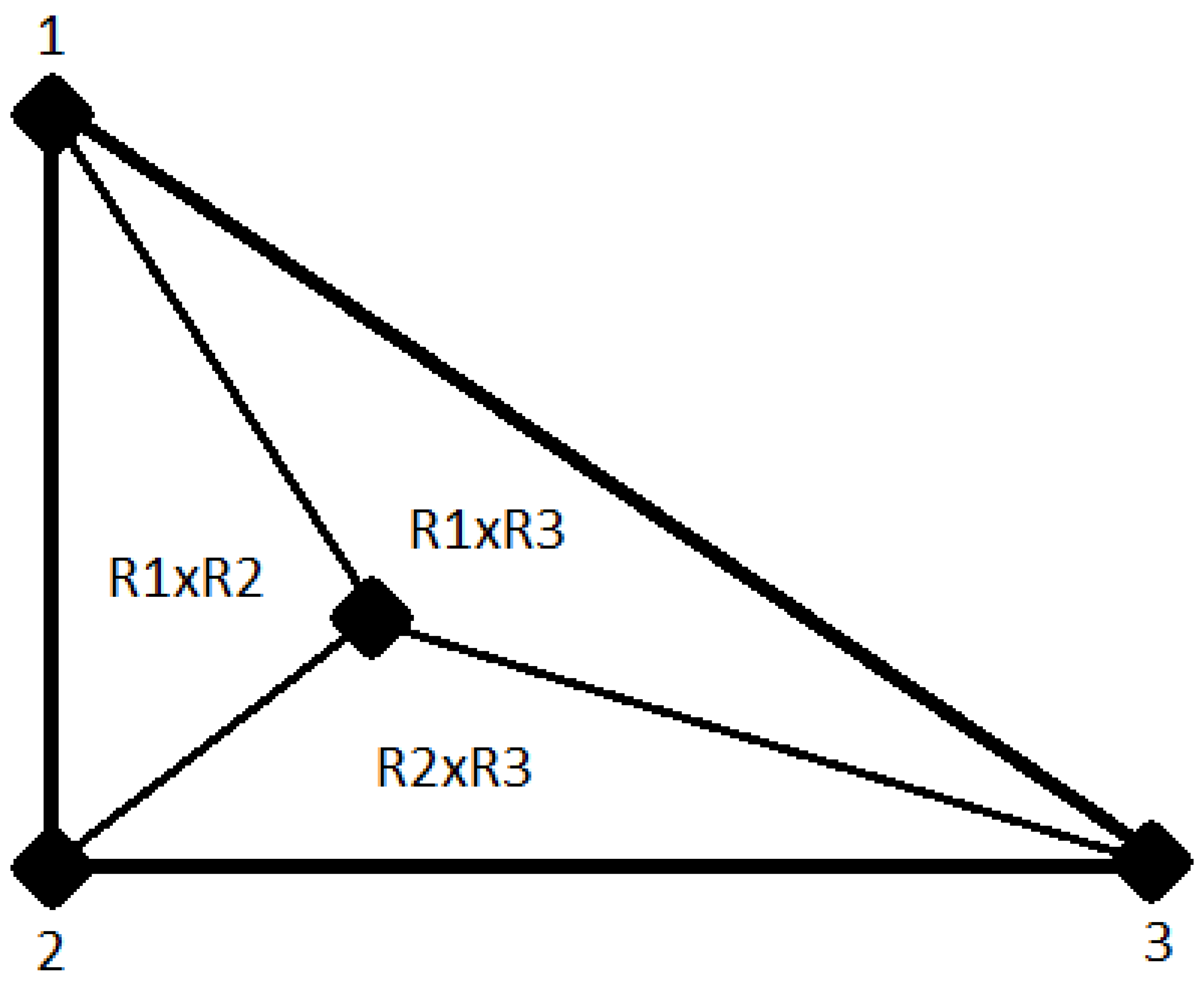
• Find the area formed by each of the three pairs of vectors three times.

  –

  $R_1\times R_2$, $R_2\times R_3$, and $R_1\times R_3$, where $R_1$, $R_2$, and $R_3$ represent the vector formed in between the centroid and node 1, 2, and 3, respectively.

  –

  The area is calculated as half of the absolute value of the cross product of the two vectors, to form each smaller triangle

  $$\begin{array}{ccc}\hfill A& =& \frac{1}{2}·|R_1\times R_2|\hfill \\ & =& \frac{1}{2}·\{{(R_{1B}·R_{2C}-R_{1C}·R_{2B})}^2+{(R_{1A}·R_{2C}-R_{1C}·R_{2A})}^2+{(R_{1B}·R_{2A}-R_{1A}·R_{2B})}^2\},\hfill \end{array}$$

  (4)

  where $R_1$ and $R_2$ are vectors of components A, B, and C.

• The areas of these three small triangles is added up to determine the area of the larger triangle (Figure 1)
• If the element surface is a quad, this process is performed twice, treating the quad as two triangles

  –

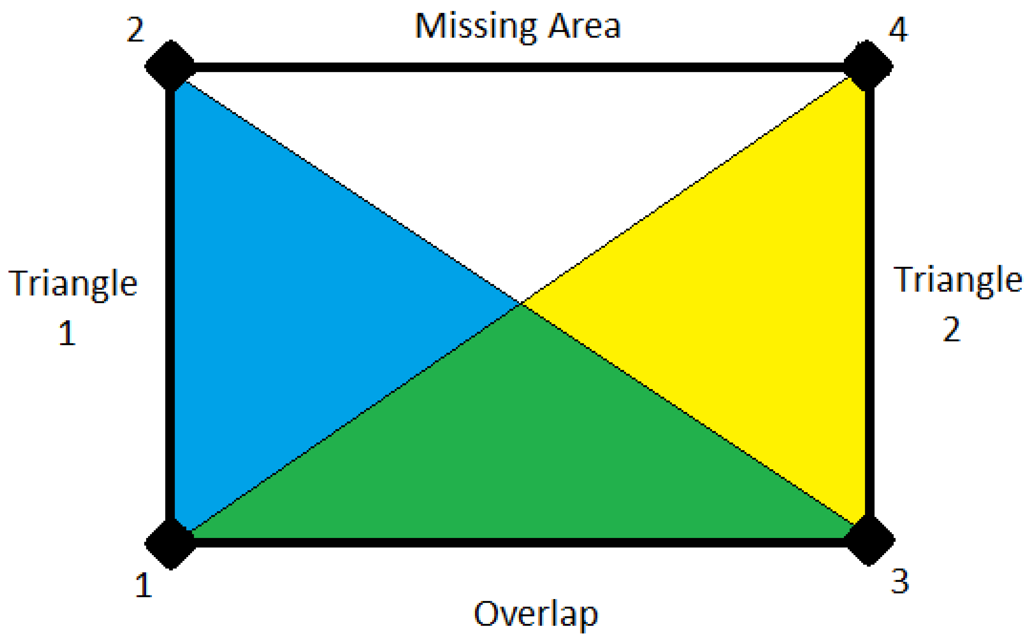
  Different software packages use different node patterns. If the wrong pattern is used, the area could be erroneously calculated (Figure 2),

  –

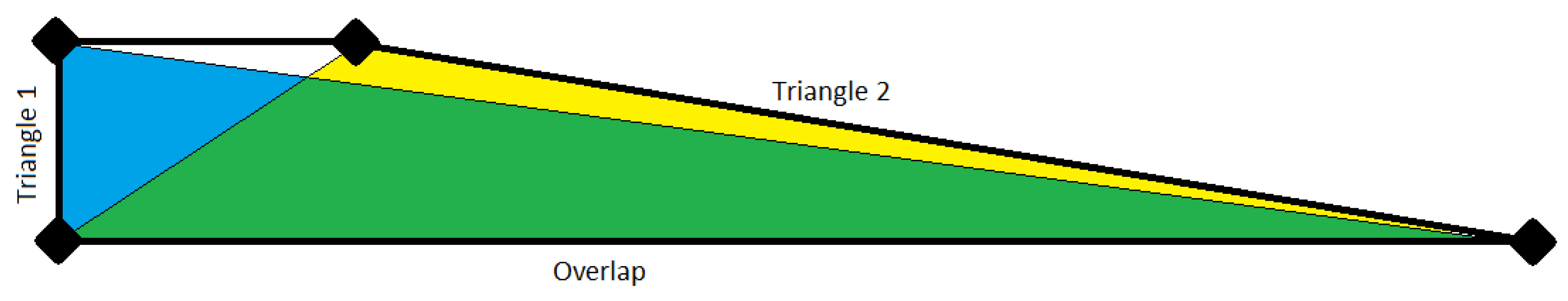
  It is not an option to find the node the greatest distance away, as an oddly shaped element would give an erroneous calculation (Figure 3),

  –

  The areas of all three combinations of two possible triangles are calculated (

  Table 1. Three different areas of two triangles; the maximum total area represents the correct area of the quad element face.

  Quad Area	Node (First Triangle)	Node (Second Triangle)
  Area 1	Node 1, 2, 3	Node 1, 2, 4
  Area 2	Node 1, 3, 2	Node 1, 3, 4
  Area 3	Node 1, 4, 2	Node 1, 4, 3

  ),

  –

  The maximum of these three possible areas is selected as the area of the quad of interest.

The next step is to calculate the normal vector of each element. In addition to weighting the source-to-target impact by distance between centroid, this approach also considers the angles of each surface. If a source surface is parallel to a target surface, then the force may be fully applied; if the elements’ surfaces are perpendicular, then there is no impact of the source on the target. The normal vector is found by normalizing the cross product of the vectors between Node 1-2 and Node 1-3. It would not matter if the element surface was a quad or a triangle, or what order the nodes were located; assuming the surface is flat as would be the case for a linear element, then any combination of node vectors should yield the unit normal.

3. Algorithm

Once it is defined what the centroid, surface area, and unit normal vector is for each source and target element, the mapping algorithm can commence. The goal of mapping is to determine how much of an impact each source element will have on each target element. If there is perfect overlap from a source and an element, then all of the force from that source element will be applied to that target element. Of course, in practice, this almost never happens, and therefore a weighting scheme is needed to determine what proportion of each source element is applied to each target element. The impact of a source onto a target can be defined as W, a dimensionless number from 0 to 1; a value of 0 means there is no force from the source applied to the target, and a value of 1 means all of the force from the source is applied to the target.

The first step is to look at the distance from centroid to centroid, and the relative impact $W_r$. A magnitude function should be one where the magnitude decreases exponentially with distance, such as the Gaussian function

$$\begin{array}{ccc}\hfill W_r& =& exp(-\frac{r}{h}),\hfill \end{array}$$

(5)

where r (m) is the linear distance from the source centroid to the target centroid, and h (m) is the smoothing value. The value should be such that $W_r$ is small if the distance between centroids is so great that the source element is completely outside of the target element. It was found that good results came from setting h to equal the mean average value of the square root of the target element areas.

The second aspect of the impact $W_A$ between source and target elements is the angle separating the unit normal for each element. This value can be found by taking the dot product of the unit normal vectors:

$$\begin{array}{ccc}\hfill W_A& =& V_S·V_T=V_{S,x}·V_{T,x}+V_{S,y}·V_{T,y}+V_{S,z}·V_{T,z},\hfill \end{array}$$

(6)

where $V_S$ and $V_T$ are the unit-normal vectors for the source and the target element. If the two elements are perfectly parallel, then $W_A$ = 1. Even if the centroids of a target element are proximate, if they face perpendicular to each other they ought to not have any impact with each other and $W_A$ = 0. In practical application, if the surfaces are identical, proximate elements should be very close to parallel to each other; only distant source elements might be significantly less parallel, and they will have a low value of $W_r$ so that the value of $W_A$ should be irrelevant. The importance of this step, however, is when there are sharp edges in a 3D, model; such source elements might have dramatically different directions and therefore should have little impact, yet be proximate to a target element. For this reason, both the separation distance as well as the normal vectors of each source and target vectors are considered to get a total dimensionless weighting value

$$\begin{array}{ccc}\hfill W& =& W_r·W_A,\hfill \end{array}$$

(7)

where W, a dimensionless value between 0 and 1, is the weighted impact value of a source and a target.

This approach is performed for source and target pair, and is the most computationally intensive task of the mapper, requiring $N_S·N_T$ distance calculations, where $N_S$ and $N_T$ are the number of sources and targets. For typical models of hundreds of thousands of surface elements, an $N_S·N_T$ array would take up far more memory than most computers can handle, and therefore an optimizing approach is necessary. The first step is categorizing the targets that each source can have a meaningful amount of impact with; this is stored in two $N_S·N_X$ arrays, where $N_X$ is an arbitrarily small, user defined integer value (typically 5 to 10). The first array defined as a real variable array of the impact value W; the second is defined as an integer array and represents the target the specific source impacts. For each source element, the impact magnitude of all of the targets was found. To keep the number of contacted targets within the value of $N_X$, the calculated impact magnitude was only stored in the array if the value was greater than the minimum of all $N_X$ impact magnitudes stored. If it was greater than the minimum, the calculated value was stored in the array location of the previous minimum impact value; the target element number was stored in the equivalent location in the integer array. This method serves the goal of finding the top $N_X$ target elements that have the greatest impact magnitude W to a given source.

One potential issue that can come up with mapping is the potential for target elements to have no proximate source elements. This is especially possible from different geometries or meshes. A user may prefer to map every target with the nearest mesh, regardless of how far it is; this will, however, result in pressures not actually applied on the target being predicted. Another option is for the user to set a minimum value of the impact magnitude W. This has the advantage of preventing pressures far from a target element from impacting the final pressure calculation; there is the risk (possibly desired by the user) that some target elements fail to get meshed by any source elements. There is another advantage that, since the vast majority of target elements will be too far from the source element of interest to have an impact magnitude W exceed the minimum value of W, all these calculated values are not written to memory, significantly reducing run time for large meshes.

After this step has been completed, each of the $N_S$ source elements have $N_X$ or less target elements with a varying impact magnitude of W ranging from 0 to 1. The calculated value of W is fairly arbitrary, and the smoothing function can be modified by the user. What cannot be arbitrarily altered is the total summation of the forces; the total forces must match in the transfer matrix. With each source, the actual impact of all $N_X$ proximate target elements are normalized $W_N$, so that

$$\begin{array}{ccc}\hfill {\mathsf{\Sigma }}_{i=1}^{N_X}{W}_{N,i}& =& 1.\hfill \end{array}$$

(8)

These normalized impacts represent the proportion that the force from one source element is applied to a given target element. This approach enables that the total force from each source is equally applied to $N_X$ target elements, and the cumulative forces match for both the source and the target.

The transfer matrix does not work in terms of force but of pressure; the goal of the mapper is to find an even distribution of source pressures that combine to a given target element. To determine the magnitude of a source pressure on a target element $W_P$, the ratio of the element areas are applied, and thus

$$\begin{array}{ccc}\hfill W_P& =& W_{N,i}·\frac{A_S}{A_{T,i}},\hfill \end{array}$$

(9)

where $A_S$ is the area of the source, $A_{T,i}$ is the area of the specific target, $W_{N,i}$ is the normalized ratio of the force from the source that is applied to target i, and $W_P$ is the ratio of how much pressure from the source is added to the total pressure of target i.

The last and final step is to swap the calculated values of $W_P$ from a $N_S·N_X$ array to a $N_T·N_{X2}$ array, where $N_{X2}$ is an integer value significantly greater than $N_X$. This is simply determined by

• Sorting through the $N_S·N_X$ array of $W_P$ for each source element,
• Adding to the target number found, the location in a $N_T·N_{X2}$ array,

  –

  That source element, the source element number, and the pressure magnitude data $W_P$.

• Incrementing the count of sources proximate to a given target

  –

  Stored in a separate integer vector ($N_T·1$),

  –

  Used to track how many source elements are proximate to the given target element,

  –

  Can be expected to exceed $N_X$ provided the number of source elements is greater than the number of target elements,

  –

  Should never exceed $N_{X2}$; if this happens, it is necessary to increase the value of $N_{X2}$ to avoid memory errors,

• Save the transfer matrix.

Saving the transfer matrix is the last and final step. This algorithm saves the transfer matrix as a separate output file for the combination of two specific meshes; the actual pressure is irrelevant. The transfer matrix by definition is the proportion of all the source pressures that make up each target pressure, so that the cumulative forces all match. The purpose of saving this transfer matrix is so that, in the future, a host of different pressures can be mapped onto the surface without needing to rerun the computationally expensive mapping script. In practice, a numerical analysis will run in many time-steps, and one might want to map a host of different pressures to the same mesh. The format of the output transfer matrix includes:

• Number of elements $N_T,$

  –

  This number is saved so a future mapping algorithm knows the number of target pressures to generate,

• For $N_T$ times, list the specific target and the following information,

  –

  Target number, Number of Sources Proximate, and Sum of Pressure Impacts $W_P$

  –

  The reason for the sum of $W_P$ is because each individual value of $W_P$ is normalized by the cumulative sum of $W_P$ for all proximate targets, so that the pressure of the target element is a proportional average of these proximate source elements.

• For each target, for the number of proximate source elements,

  –

  Sequential number, source element number, and pressure impact $W_P$

4. Test Example

To demonstrate the robustness of this mapping algorithm, an arbitrary mapped source mesh will be mapped onto a target, for 180 different pressures; the details of this code are described in the Appendix A, and included in the Supplementary file. The source is a grid of 450·450 nodes, spanning from −0.1 to 1.1 in the X, Y, and Z direction; the grid is slanted along the Z plane so that Z = Y. All of the elements are the quads formed by the 202,500 nodes, resulting in ${(450-1)}^2=$ 201,601 source elements. The target domain is smaller, stretching from 0 to 1 in the X, Y, and Z direction, also parallel to the Z plane, and these nodes are an even grid of 225·225 = 50,625 nodes. Different from the source, which uses exclusively quad surface elements, the target has a mix of quads and triangles. Moving up in the Y and Z direction, odd numbered rows are all quads, whereas even numbered rows are all triangles, with two triangle surface elements formed per four nodes.

An arbitrary pressure was applied to 180 time steps, all with different pressures. The pressure for a given time step is

$$\begin{array}{ccc}\hfill P(x,y)& =& (C_X·x{x}^2)+(C_Y·y{y}^2)+P_{spot},\hfill \end{array}$$

(10)

where

$$\begin{array}{c}\hfill xx=x+(\frac{oo}{180}·1.2),\\ \hfill yy=y+(\frac{oo}{180}·1.2),\\ \hfill C_X=500+2·oo,\\ \hfill C_Y=1500-3·oo,\end{array}$$

(11)

and oo is the time step, ranging from 1 to 180. If xx or yy ever exceeded the value of 1.1, then xx or yy was subtracted by 1.2. This will cause a moving pressure boundary in the X and Y direction, demonstrating the robustness for sudden pressure changes. In addition, a Gaussian pressure spike is added at a cyclic location

$$\begin{array}{c}\hfill P_{spot}=5000·exp(-10·rr),\\ \hfill rr=\sqrt{{(x-X_C)}^2+{(y-Y_C)}^2},\end{array}$$

(12)

where

$$\begin{array}{c}\hfill X_C=0.5+0.25·cos(\frac{oo·\pi }{90}),\\ \hfill Y_C=0.5+0.35·sin(\frac{oo·\pi }{90}).\end{array}$$

(13)

The mapping was completed, and, for all 180 time steps, the cumulative forces matched almost exactly (Figure 4). The forces shown in Figure 4, representing the integrated pressures over area such as in Figure 5, are of arbitrary units; this example uses pressures in Pascals, applied over a surface area of one square meter, to give the force in Newtons. Obviously, the total forces for the source is greater, as the surface area for the source is greater, but, by isolating all of the elements within the range of 0 to 1 meter that will be applied to the target mesh, the target force matches nearly perfectly for all of the pressure steps.

When looking at the individual mapped surfaces such as in Figure 5, it is clear that sharp lines, high peaks, and random pressure spikes are unaffected, and the mapped pressures on the target closely match the mapped pressures on the source.

5. Conclusions

A robust algorithm has been demonstrated to map pressures from a source shell mesh onto a surface target of a similar geometry but of a different mesh. This algorithm has been tested to work with both quads and triangles, and both geometries work. After mapping two dramatically different meshes, with different overall geometries, different structured elements, and significantly different sizes, forces and pressure profiles have managed to consistently match. This test demonstrates the effectiveness of using this method to robustly map pressures from one mesh onto another.

References

1. Haberman, R. Applied Partial Differential Equations with Fourier Series and Boundary Value Problems, 4th ed.; Prentice Hall: Upper Saddle River, NJ, USA, 2003. [Google Scholar]
2. Nagel, R.K.; Saff, E.B.; Snider, A.D. Fundamentals of Differential Equations, 5th ed.; Addison Wesley: Boston, MA, USA, 1999. [Google Scholar]
3. Garcia, A. Numerical Methods for Physics, 2nd ed.; Addison-Wesley: Boston, MA, USA, 1999. [Google Scholar]
4. White, F. Fluid Mechanics, 5th ed.; McGraw-Hill: Boston, MA, USA, 2003. [Google Scholar]
5. Cengel, Y. Heat Transfer, a Practical Approach, 2nd ed.; Mcgraw-Hill: New York, NY, USA, 2002. [Google Scholar]
6. Banerjee, D.K. Software Independent Data Mapping Tool for Structural Fire Analysis. NIST Tech. Note 2014, 1828, 1–45. [Google Scholar]
7. Smith, W.G.; Ebert, M.P. A Method for Unstructured Mesh-to-Mesh Interpolation; Hydromechanics Department Report; NSWCCD-50-TR-2010; Naval Surface Warfare Center Carderock Division: Bethesda, MD, USA, 2010; p. 056. [Google Scholar]
8. Tang, T. Moving Mesh Methods for Computational Fluid Dynamics. Contemp. Math. 2005, 383. [Google Scholar] [CrossRef]
9. Budd, C.J.; Huang, W.; Russell, R.D. Adaptivity with Moving Grids. Acta Numer. 2009, 18, 111–241. [Google Scholar] [CrossRef]
10. Gao, Q.; Zhang, S. Moving Mesh Strategies of Adaptive Methods for Solving Nonlinear Partial Differential Equations. Algorithms 2016, 9, 86. [Google Scholar] [CrossRef]
11. Budd, C.J.; Williams, J.F. Moving Mesh Generation Using the Parabolic Monge–Ampere Equation. SIAM J. Sci. Comput. 2009, 31, 3438–3465. [Google Scholar] [CrossRef]
12. Wang, W.; Yan, Y. Strongly coupling of partitioned fluid-solid interaction solvers using reduced-order models. Appl. Math. Model. 2010, 34, 3817–3830. [Google Scholar] [CrossRef]
13. Basting, S.; Quaini, A.; Canic, S.; Glowinski, R. Extended ALE Method for fluid-structure interaction problems with large structural displacements. J. Comput. Phys. 2017, 331, 312–336. [Google Scholar] [CrossRef]
14. Farhat, C.; van der Zee, K.G.; Geuzaine, P. Provably second-order time-accurate loosely-coupled solution algorithms for transient nonlinear computational aeroelasticity. Comput. Methods Appl. Mech. Eng. 2006, 195, 1973–2001. [Google Scholar] [CrossRef]
15. Degroote, J.; Haelterman, R.; Annerel, S.; Bruggeman, P.; Vierendeels, J. Performance of partitioned procedures in fluid-structure interaction. Comput. Struct. 2010, 88, 446–457. [Google Scholar] [CrossRef]
16. Wick, T. Fluid-structure interactions using different mesh motion techniques. Comput. Struct. 2011, 89, 1456–1467. [Google Scholar] [CrossRef]
17. Amsallam, D.; Farhat, C. An Online Method for Interpolating Linear Parametric Reduced–Order Models. SIAM J. Sci. Comput. 2011, 33, 2169–2198. [Google Scholar] [CrossRef]
18. Amsallem, D.; Zahr, M.; Choi, Y.; Farhat, C. Design optimization using hyper-reduced-order models. Struct. Multidiscip. Optim. 2015, 51, 919–940. [Google Scholar] [CrossRef]
19. Assessment of Computational Fluid Dynamics (CFD) for Nuclear Reactor Safety Problems; NEA/CSNI/R(2007)13 OECD Nuclear Energy Agency: Le Seine Saint–Germain—12, boulevard des Illesm F-92130 Issy-les-Moulineaux, France, January 2008. Available online: https://inis.iaea.org/search/search.aspx?orig_q=RN:44037880 (accessed on 11 June 2019).
20. Lee, Y.; Gwak, M.C.; Cho, H.; Joo, H.S.; Shin, S.J.; Yo, J.J.; Shin, J.C. Numerical Simulation of Fluid Structure Interaction Problem Associated with Vertical Launching System. J. Spacecr. Rockets 2018, 55, 948–958. [Google Scholar] [CrossRef]
21. Cirak, F.; Radovitzky, R. A Lagrangian Eulerian shell fluid coupling algorithm based on level sets. Comput. Struct. 2005, 83, 491–498. [Google Scholar] [CrossRef]
22. Tremel, U.; Sorensen, K.A.; Hitzel, S.; Rieger, H.; Hassan, O.; Weatherill, N.P. Parallel remeshing of unstructured volume grids for CFD applications. Int. J. Numer. Methods Fluids 2007, 53, 1361–1379. [Google Scholar] [CrossRef]
23. You, Y.H.; Na, D.; Jung, S.N. Data Transfer Schemes in Rotorcraft Fluid–Structure Interaction Predictions. Hindawi Int. J. Aerosp. Eng. 2018, 2018, 3426237. [Google Scholar] [CrossRef]
24. Samareh, J.A. Discrete Data Transfer Technique for Fluid–Structure Interaction. In Proceedings of the 18th American Institute of Aeronautics and Astronautics Computational Fluids Dynamics Conference, Miami, FL, USA, 25–28 June 2007. Session: CFD–17: Fluid–Structure Interaction. [Google Scholar] [CrossRef]
25. Guruswamy, G.P. A review of numerical fluids/structures interface methods for computations using high-fidelity equations. Comput. Struct. 2002, 80, 31–41. [Google Scholar] [CrossRef]
Figure 1. Triangle element face divided into three parts.
Computation 07 00029 g001
Figure 2. An example of how picking the wrong nodes to divide a quad into two triangles (blue and yellow) can cause error due to area overlap (green), utilizing nodes 1-2-3 and 1-3-4.
Computation 07 00029 g002
Figure 3. Another example of how picking the wrong nodes to divide a quad into two triangles (blue and yellow) can cause error due to area overlap (green), demonstrating how an assumption cannot be made by searching for the longest vector between two nodes.
Computation 07 00029 g003
Figure 4. Comparison of the Total Forces in Newtons of the source versus the target, for 180 different source pressure profiles.
Computation 07 00029 g004
Figure 5. Comparison of the Pressures of one time step, both Source and Target, for oo = 100. The color-bar represents the pressure (Pa).
Computation 07 00029 g005