3. The LSTMs Forecasting Framework: Description
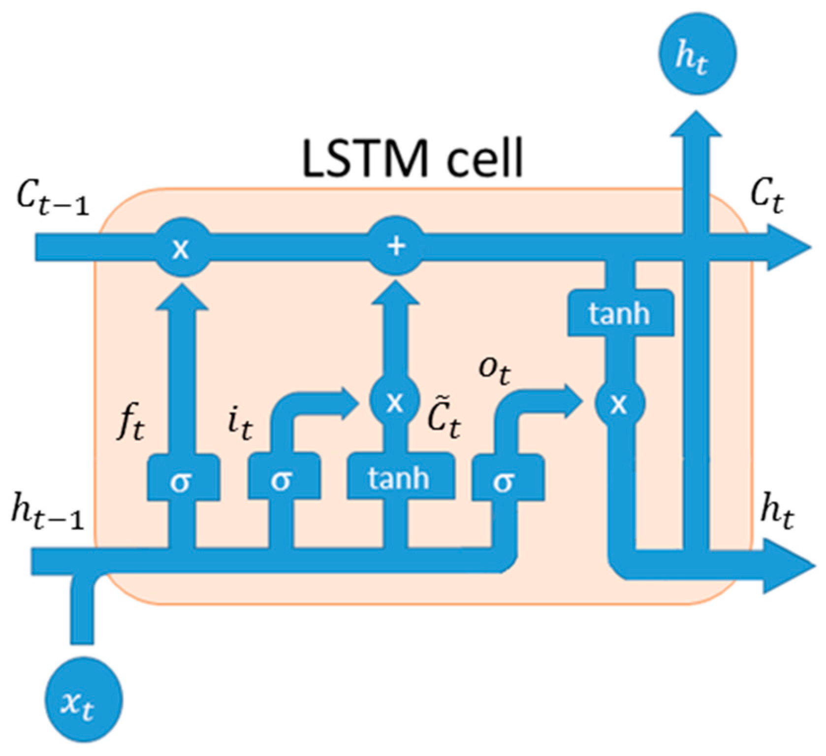
Our prediction framework is composed by two LSTM networks: One for trend prediction and another one for stock close price time-series regression. The first implemented LSTM network is used for stock trend forecast: it is basically composed of an input layer in which we fed one stock close price value at once; an hidden layer of 400 neurons and finally a fully connected output layer (one neuron). The second LSTMs layer shows the same structure, but some configuration parameters and training updates are different because it will be used for stock close price prediction. To validate the method, we decided to select historical data (Daily timeframe) about bank stocks (e.g., Unicredit [UCG.MI], Monte dei Paschi di Siena [MPS.MI], Intesa San Paolo [ISP.MI], and Credito Valtellinese [CVAL.MI], etc.), as well as a corporate share i.e., Enel [ENEL.MI], all listed in the Milano Stock Exchange Market. All daily data have been downloaded from Yahoo Finance website [
14]. The historical data have been collected from October 2000 to October 2018 and each entry is referred to daily timeframe. Specifically, we collected for each share: Daily Open/Close/High/Low prices even though we validate our system only for Close prediction. All collected financial values have been arranged as part of training set and part as validation set. All values were normalized in the range (−1, 1), with classical MinMaxScaler algorithm. In
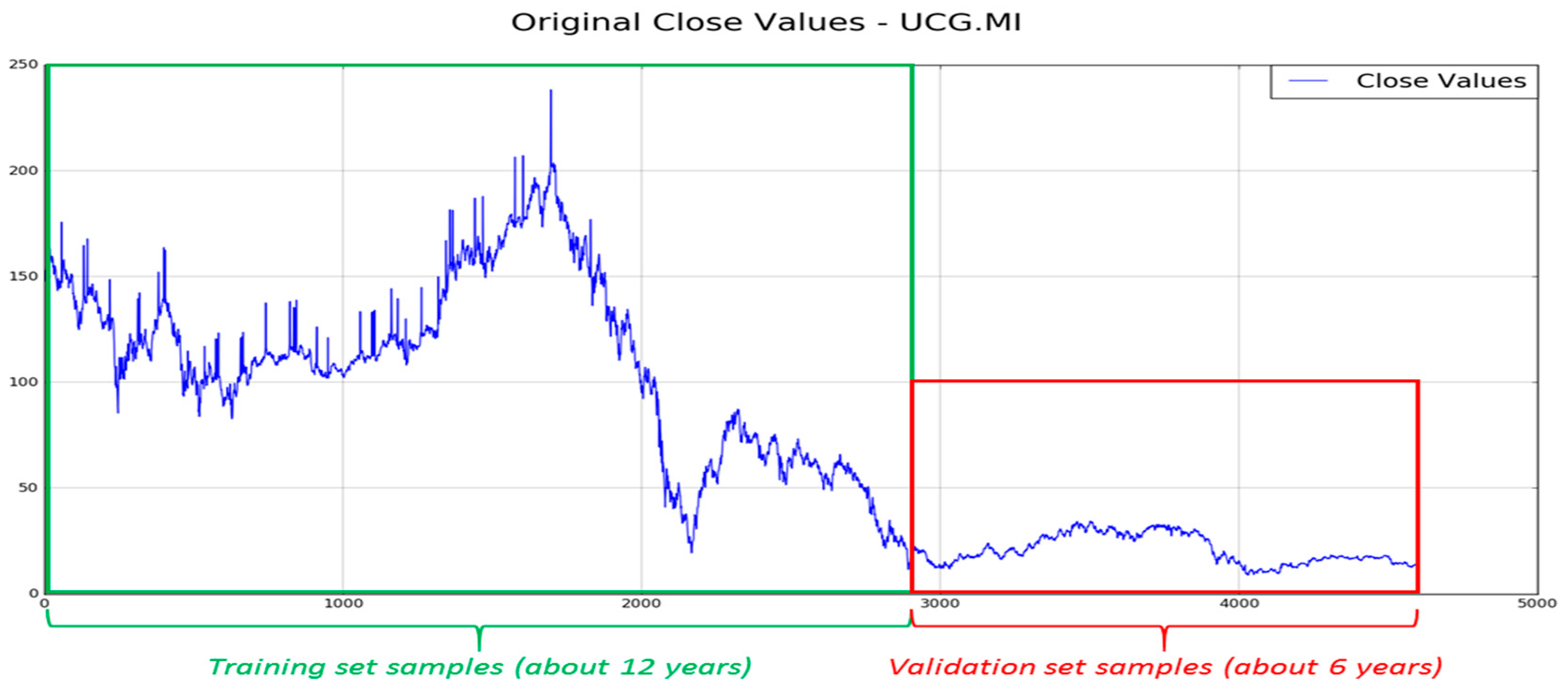
Figure 3 we show an instance of the stock included in the arranged dataset (Unicredit) in which the blue-colored part of the share timeserie represents the data we collected as training set, while the remaining ones (red-colored) is used as a test and validation set of the proposed approach. In more detail, in order to perform a valid and robust training session, we considered about 12 years of the 18 collected that denotes about 2900 input data (highlighted by green rectangle), as per previous description. The remaining six years (about 1600 data) are used as the validation set of the proposed pipeline.
In
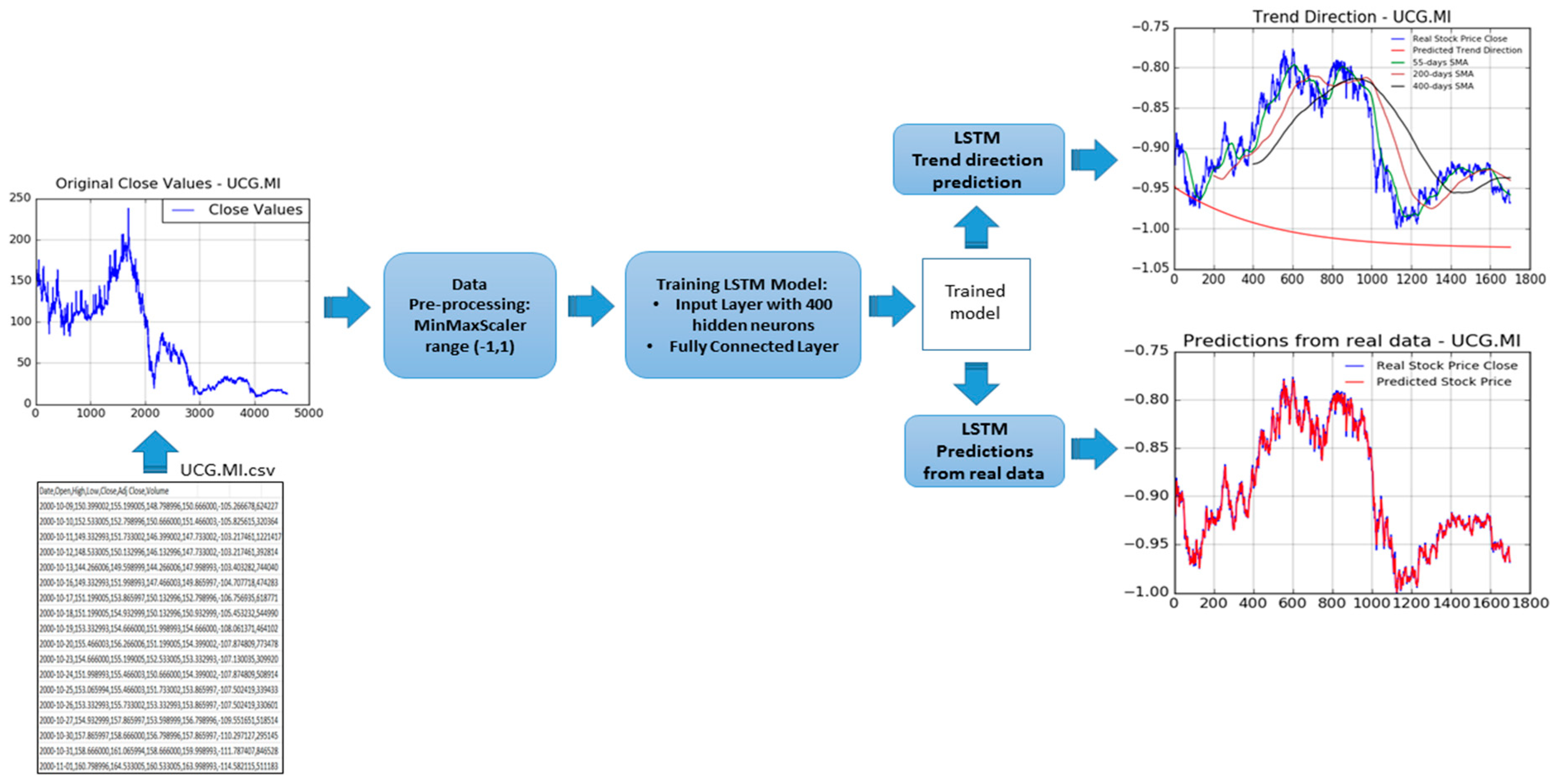
Figure 4, the authors report an overall representation of the proposed pipeline (the part devoted to the stock trend and price prediction) in order to show the processing flow we have designed to reach the desired targets: An efficient stock price and trend prediction algorithm.
The proposed stock trend and price prediction pipeline is then composed by the following components: A data pre-processing block followed by the two pipeline LSTM framework (in which one pipeline for Trend prediction and another one for stock price prediction). The first block (data pre-processing) is able to normalize input stock price timeserie data, as well as to split input data between training and validation, as above described. The so processed data are fed into LSTM framework in which it will be properly processed in order to provide an estimation of the mid-long term trend (LSTM Trend direction prediction), as well as of the stock prices (LSTM Prediction from real data). About this latest block, the proposed stock close price prediction system is based on the usage of LSTM together with mathematical price correction approach based on the usage of the so-called Markov statistical model. We introduce now a brief overview of the Markov model theory needed to understand the proposed enhanced of the LSTM prediction system. As reported in Reference [
15], the Markov Model based approaches for financial time-series forecasting shows promising results. In Reference [
15], for instance, the authors described a predicting method based on usage of Hidden Markov Model in order to improve the accuracy and a comparison of the existing techniques based on Machine and Deep learning. As is well known, a stochastic process can be defined as “Markov Process” if the underlying dynamic satisfies the Markov propriety, i.e., the probability of an event—in a well defined sequence—depends only on the state attained in the previous event. Formerly, in the discrete-time domain, if we consider a random variable
X with Markov propriety with a related probabilistic sequence
, we have:
The financial research area confirmed the fundamental role of probability theory and stochastic analysis in the share price formation. As reported in Reference [
15], in the context of stochastic analysis the Markov theory (Markov Chain, Hidden Markov Mode, Markov propriety, etc.) shows very promising results in addressing financial time series forecasting problem. More in detail, a very effective Markov based approach for addressing financial data processing issues is the assumption that price formation satisfies Markov propriety. Specifically applied in the proposed approach, the authors perform a further processing of that assumption: We assume that if the price value at specific time
yt+1 depends of previous stock price value only
yt, the related prediction error
et+1 keeps same statistics, i.e., it satisfies Markov propriety so that the current stock price prediction error
et+1 is correlated to previous ones
et only. We have applied this assumption to our prediction model based on LSTMs, as described in what follows. Formerly, we consider stock close price prediction made by the second LSTM pipeline, as pointed out in
Figure 4.
In Equation (9), we have indicated
as the stock close price at previous time
t – 1, while
represents the second LSTM prediction functional model, and then,
represents the forecasted stock close price. In our theory framework, we define
Y as the random variable describing the stock price formation under the implicit hypothesis that stock price formation satisfies Markov propriety, i.e., under the following mathematical correlation:
According to Equation (10), we have similarly supposed that the error prediction dynamic satisfies the same Markov propriety. Formerly, if we consider E as the random variable describing the prediction error evolution, the same correlation reported in Equation (9) is satisfied:
Equation (11) means, in few words, that under the adopted hypothesis (stock price prediction error dynamic satisfies the Markov propriety) we have the great advantage to use the previous prediction error
et to correct the current stock price forecasting process. Therefore, according to this clear consequence, we proceed correcting the stock close price prediction performed by our LSTM system
as per Equation (9) with a part of previous stock close price prediction error, as reported below:
where, with the parameter
p, we have defined a learning adaptive factor heuristically determined (we have configured
p = 0.5 for this work), while we have defined
as the real stock close price, and with
, the predicted ones by second LSTM pipeline (see Equation (9)). Consequently, after an appropriate training session, this part of the proposed pipeline, will be used as stock close price forward predictor. Specifically, during market evolution we select a stock and then use collected actual stock close price value at time
t for forecasting the same share close price at time
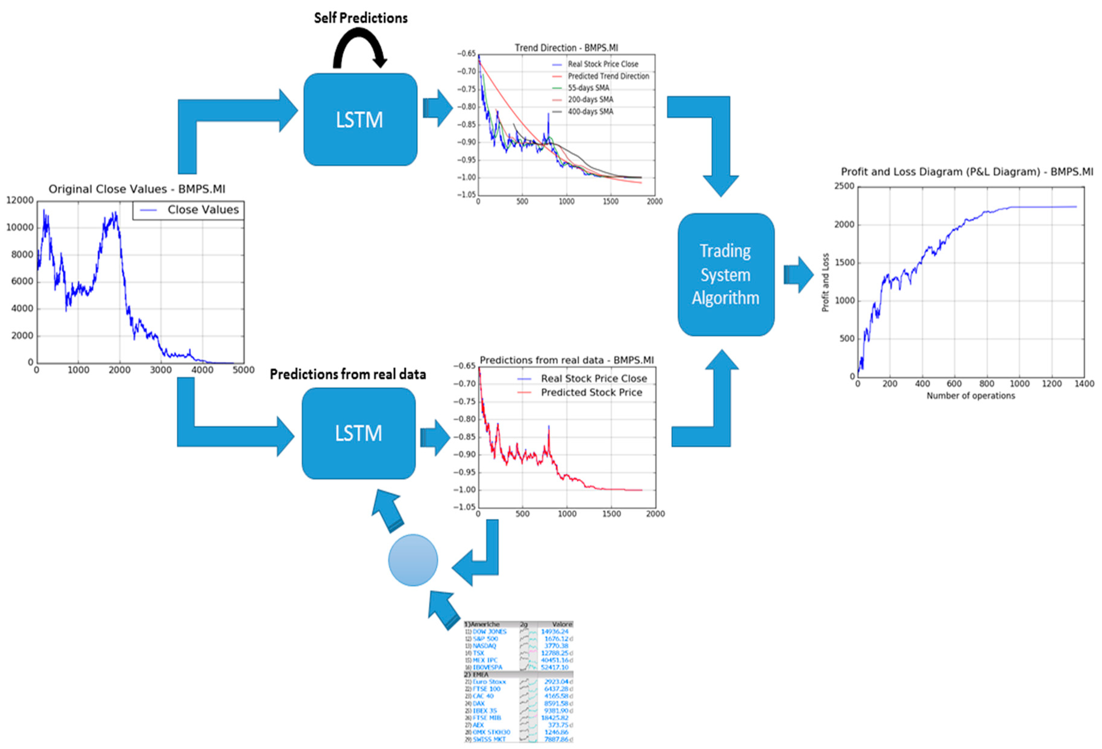
t + 1. By means of the made assumption, that price formation satisfies Markov propriety, the so obtained prediction (made by the second LSTM) will be furtherly corrected by means of the previous prediction error, as per Equation (12). Meanwhile, the first LSTM pipeline performs mid-long term trend forecast. Considering that we collect stock market prices at real time (according to adopted timeframe) we have decide to improve LSTM predictability to update the second LSTM pipeline with already collected real stock close prices. In this way, we improve the prediction accuracy of the second LSTM pipeline because we update the internal representation of the stock timeserie (acquired during the training session) with real-time data being collected. Afterwards, considering that we have predicted the mid-long stock trend as well as the next stock close price, we are ready to decide what type of financial operation to be performed. For this reason, the so predicted stock prices (from second LSTM) as well as the predicted trend information (first LSTM) will be fed into the Trading System Algorithm block to make a decision about the trade to be done (LONG vs SHORT vs Null Operation) as well as to estimate related trade parameters such as Take Profit (pre-defined amount of profit for the related trade), Stop Loss (max accepted loss for the analyzed trade), and so on. In
Figure 5, an overall scheme of the whole proposed financial pipeline is reported.
The pipeline described in
Figure 5 is a clear graphical representation of the algorithm described till now, i.e., the two LSTM pipelines for mid-long term trend prediction (Self Predictions LSTM as the deep neural network performs mid-long term trend prediction by recurrent learning of stock price timeserie without update with real data being collected) and stock close price predictions (Predictions from real data as this second LSTM—as said above—will perform a real-time update of each internal representation by using real stock prices data being collected during market session) and the new block named “Trading System Algorithm” block, which will be better described in the next section.
4. The Trading System Algorithm Block
In this section, we describe the latest block of the proposed pipeline reported in
Figure 5. In the following
Figure 6, the functional pipeline embedded in the trading system block is shown.
The first target of this block is the analysis of the mid-long term trend prediction made by the first LSTM. This analysis based on mathematical check of the LSTM output (simple derivative analysis based on the first LSTM output curve in order to understand if this curve shows growing or decreasing dynamic) will be able to provide the type of operation to be performed: LONG (buy the stock as we suppose the price will grow in the future) or SHORT (i.e., short selling as we sell the stock because we suppose the price will decrease in the future). Now, to confirm the decided LONG or SHORT operation, we proceed evaluating if the value of the predicted stock close price (by second LSTM pipeline plus Markov correction) is greater (or not) than the actual stock open price being collected from real markets. This comparison is crucial to confirm, or not, the defined operation, as previously described. Basically, we performed a LONG operation if and only if the first LSTM suggests LONG mid-long trend and the predicted stock close price is greater than the actual collected open price otherwise, the system performs a SHORT trade. The reason of the above algorithm is very simple to understand: We have a confirmation of a LONG operation if predicted stock close price is greater than the stock open price, which basically means that we suppose the stock dynamic currently pricing as per open price will grow in the future, as the predicted close price is greater than the open ones. Same reasoning but in the opposite sense, for SHORT operation. If there is a mismatch between the LSTM estimated mid-long term trend and close to open price comparison, the proposed trading system does not perform any operation (Null Operation). This decision will be done by the “Decision System” block of the pipeline reported in
Figure 6. Finally, in case of market operation (LONG or SHORT), the proposed pipeline computes the Take Profit (T/P), i.e., the amount of money you intend to gain in the opened trade. This estimation will be made in the “T/P Estimation” block. We estimate the T/P by specifying the amount of gain at which values of the system will close the trade. In order to estimate the Take Profit of the performed trade, we set the following variables:
CRV (Investment Amount): Total amount of invested money for buying or short selling the analyzed stocks.
Ns (stock numbers): Number of shares. It is obtained by means of the following formula in which we have indicated, with
yopen, the actual stock open price (13):
Cs (trade commissions): applied commissions requested by the broker or bank engaged for executing/managing requested trades. It is often defined as a percentage of the CRV. In our experiments we supposed a classical value of 0.19% to be applied to CRV both during the opening and the closing of the requested trade.
After above steps, we compute the related take profit (TP) of the requested trade at time (t), by using the following equation set (14):
where
is heuristic parameter to manage the level of profit, we defined as 0.5 in our experiments. Clearly, in (15) we report the net profit of the trade according to the broker applied commissions. After above evaluation, if all described constraints are satisfied, the proposed algorithm decides to open the trade and then to perform monitoring of the current stock price dynamic. The “P/L Computation” block is in charge to perform a time-by-time real-time Profit and Loss monitoring of the opened trade proceeding with an operation closure if the estimated take profit (TP) is reached. In case the TP is not reached, the proposed trading system performs an automatic closing of the opened trade ad the last available stock close price taking into account the related stock exchange market (in our experiment we have referred to Milan Stock Exchange Market, which close at 17.15 p.m. CET time). The above trading algorithm may be applied to any stocks or markets as well as to any timeframe. Our experiments, reported in the following section, have been conducted by selecting some stocks exchanged in the Milan Stock Exchange Market with Daily timeframe.
5. Experimental Results
In our experiments, to implement the described LSTMs framework we used Keras framework [
16]. Keras is a high-level neural networks software framework running on top of Google’s Tensorflow API framework [
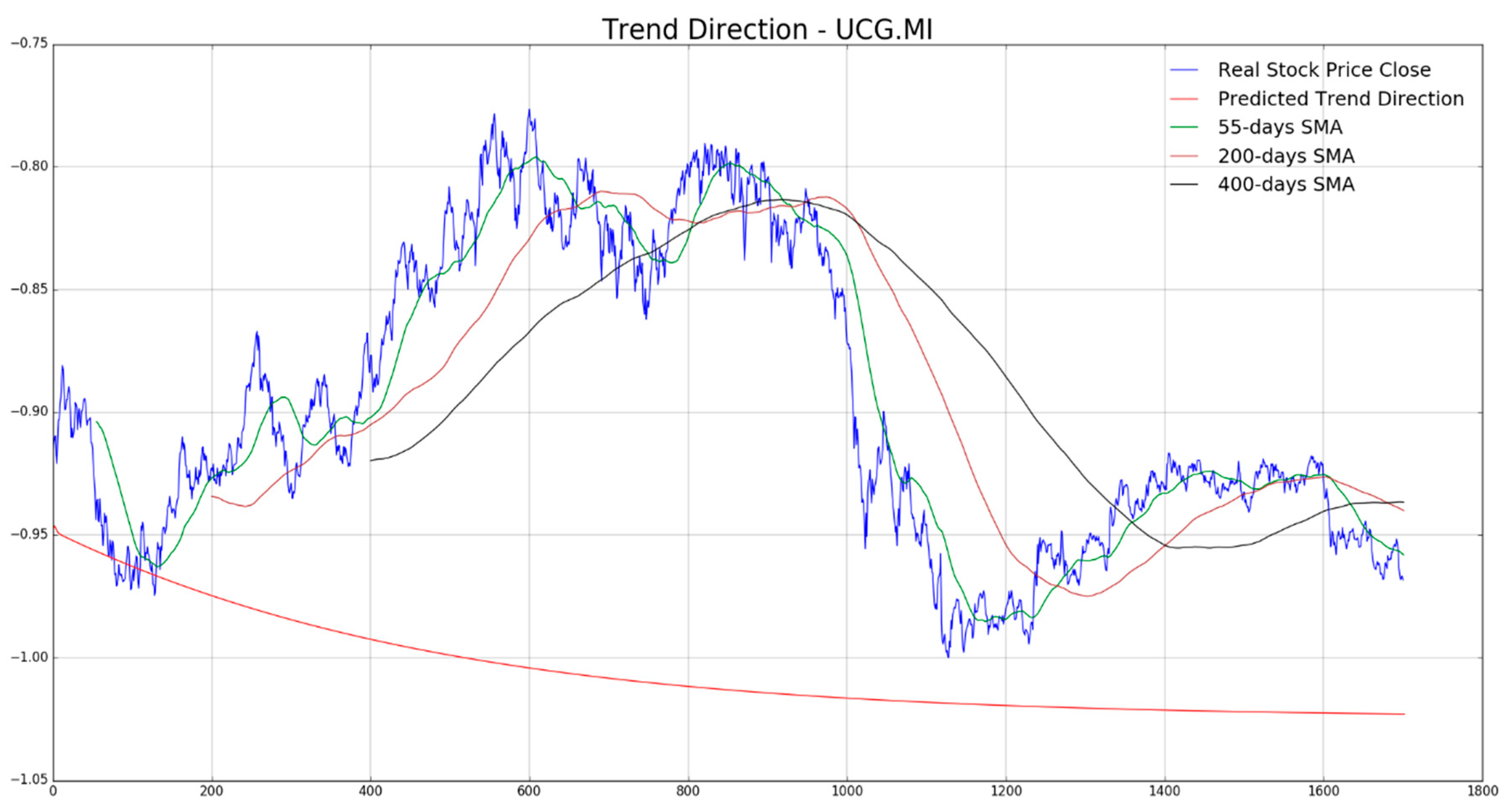
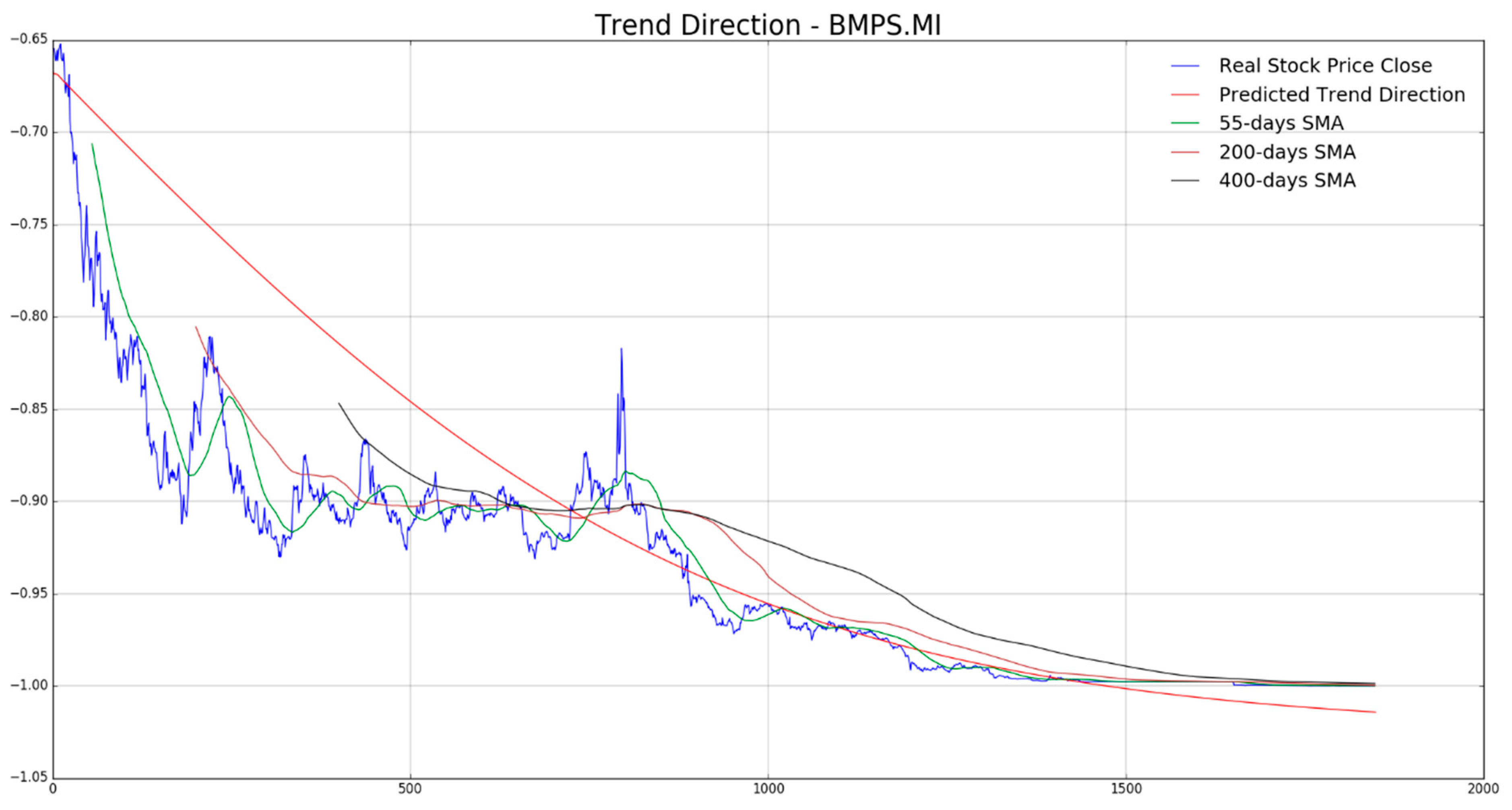
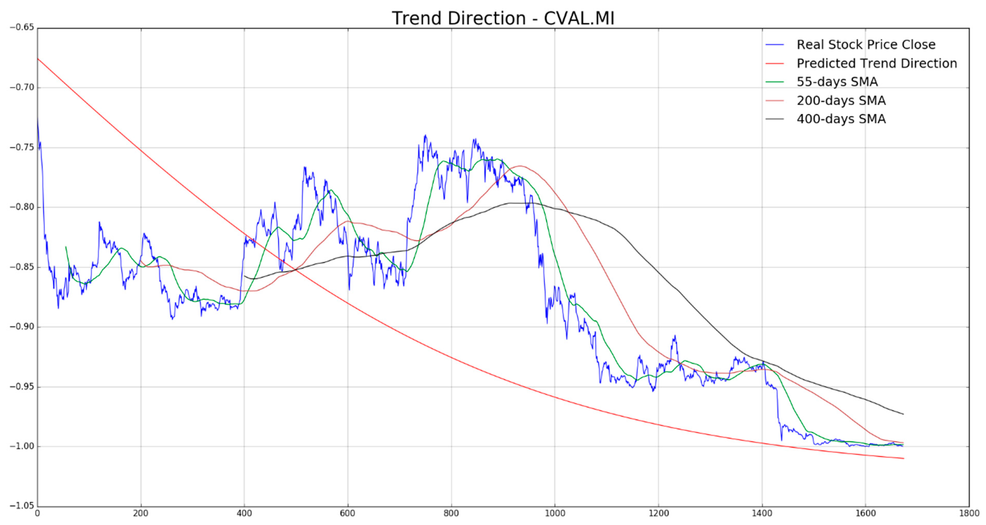
17]. Moreover, we decided to use Python library for implementing LSTM model. The experiments were executed on a PC Intel i5 quad-core with 16 Gb of RAM and 1 Tb of storage. Several experiments were carried out in order to predict the trend direction of each stock. In the following figures we report several benchmark visual comparisons of the proposed system. In each figure, we report the stock timeserie, in the analyzed period, with such analytic financial indicators (better described in the following paragraphs), as well as with first LSTM mid-long term trend prediction.
In
Figure 7,
Figure 8,
Figure 9,
Figure 10 and
Figure 11 the authors report, for each diagram, the real stock trend (blue time-serie) with the predicted trend-line (red curve). For the sake of comparison, we reported such common mathematical heuristic financial indicator such as the Simple Moving Average (SMA) over different periods in order to perform a correct discrimination of the medium and long-term stock trend. As is well known, prediction of the stock price trend, especially mid-long term trend prediction, is a great challenge as per the complexity of that market usually affected by chaotic and unpredictable dynamics. For the reasons previously described, a zero-fault pipeline that is able to predict stock trend is very difficult to obtain. In that field, the proposed approach shows promising results even though there is, of course, a great amount of work to be done for improving the obtained performance in trend prediction. In our experiments, we have noted that for such stock the mid-long term trend prediction seems accurate (see
Figure 8 and
Figure 9), while the remaining ones (
Figure 7,
Figure 10, and
Figure 11) shows a real trend not very compliant with the predicted ones likely due to such financial complex dynamic and market information not yet included in the LSTM learning, which is basically based to price movement dynamic only. Anyway, the trading system we have described in
Section 4, is able to compensate the above displacements in trend prediction, as confirmed by the good results we report in the following figures. As described in the previous
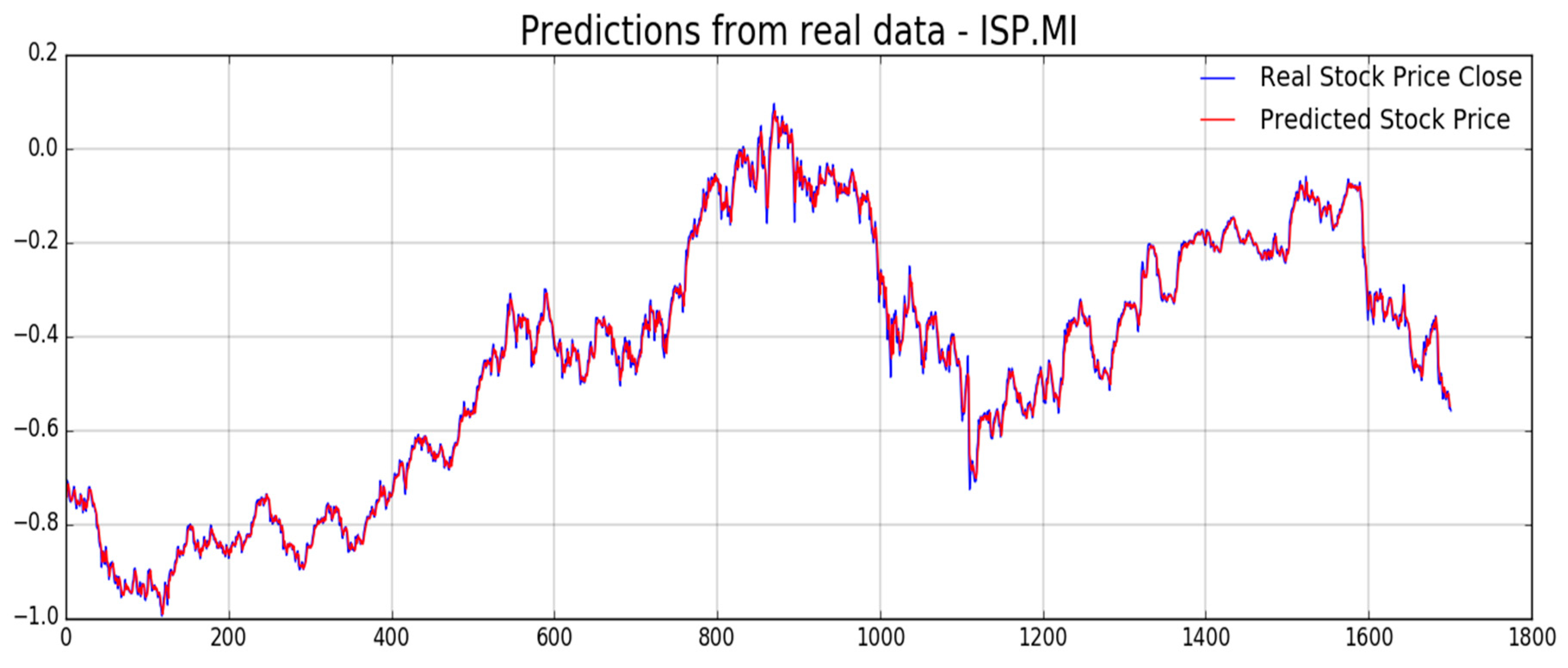
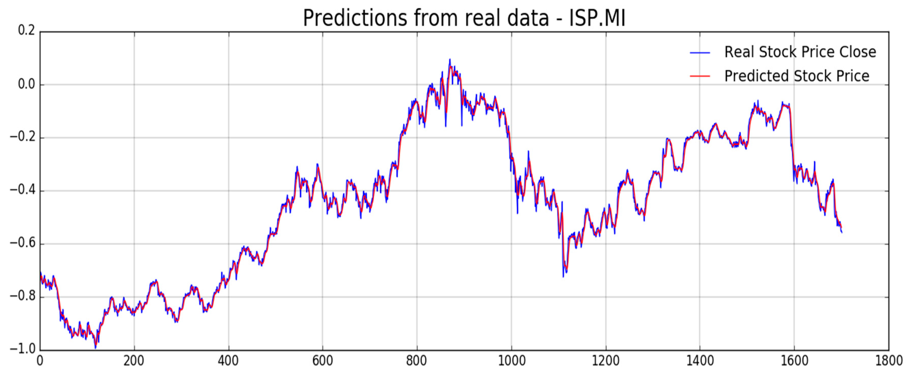
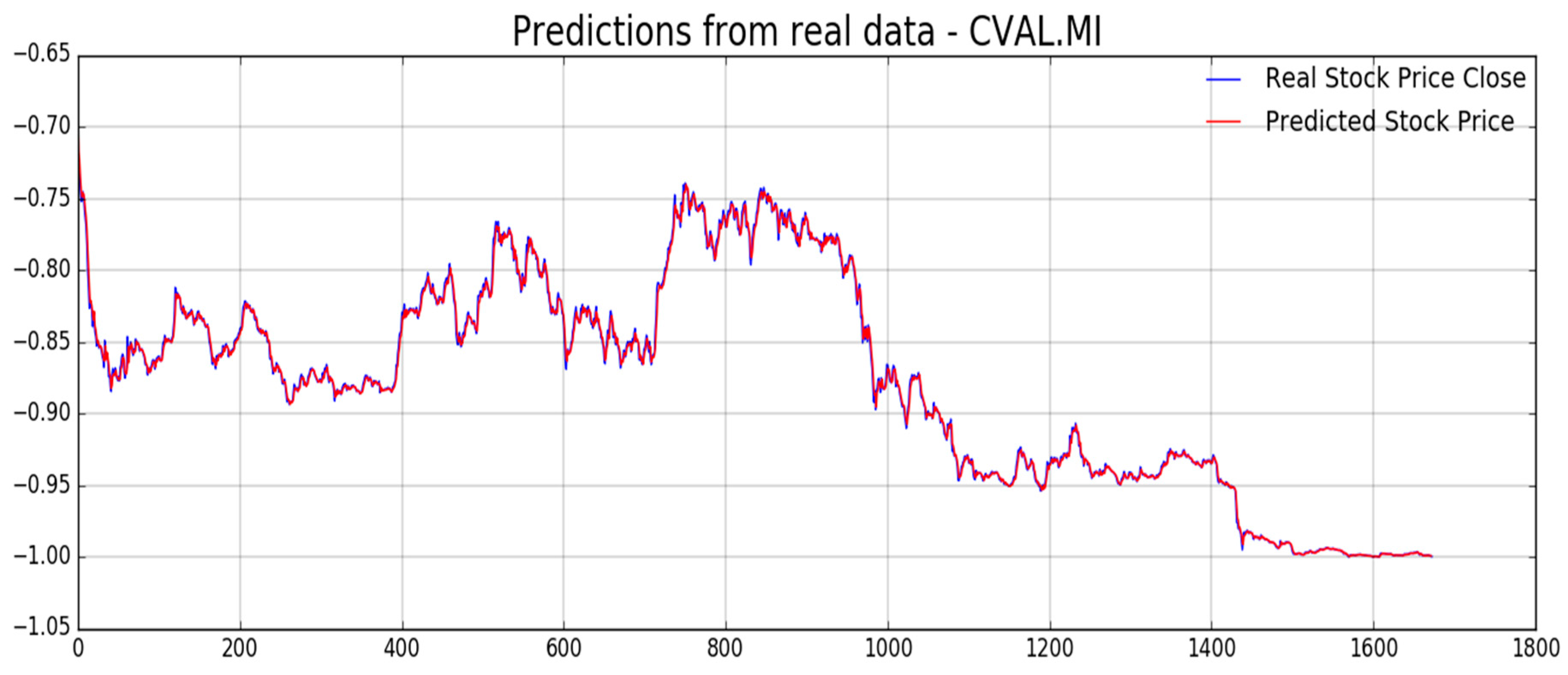
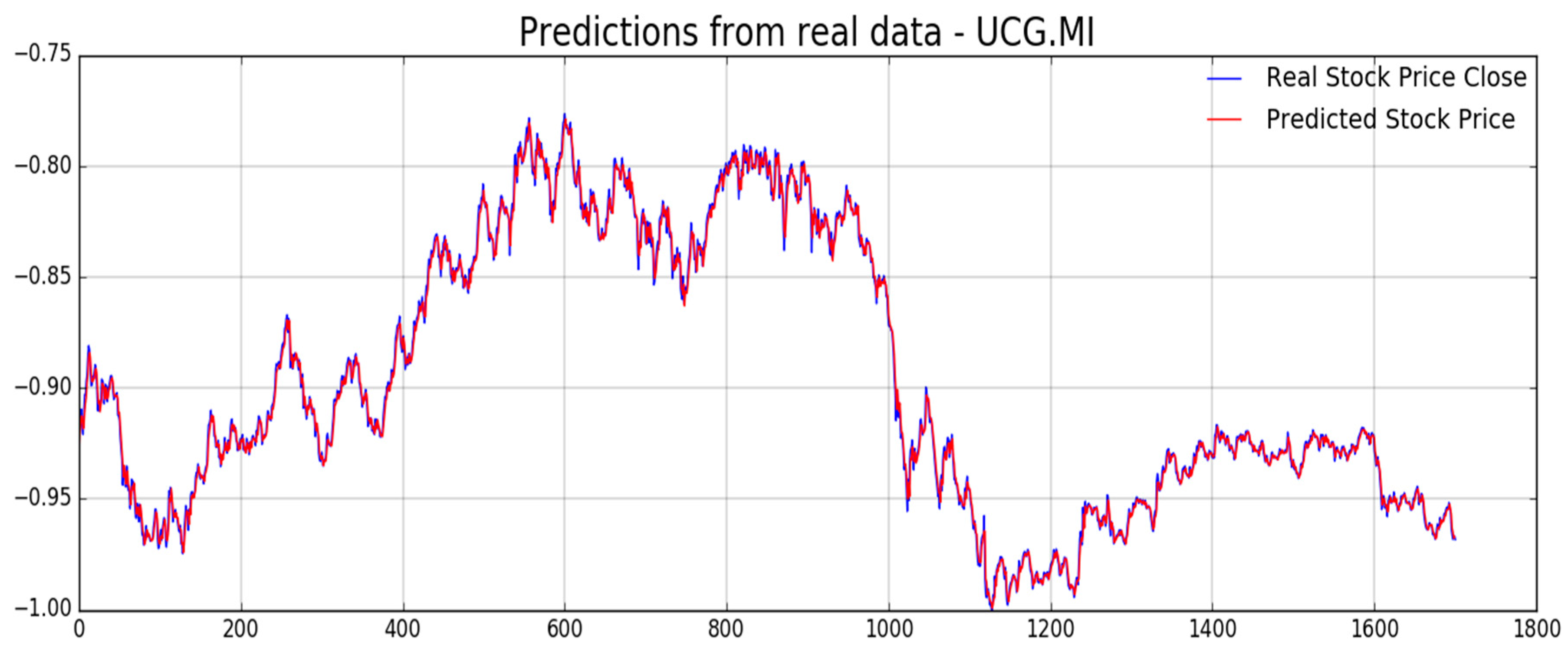
Figure 5, the proposed pipeline includes another LSTM based block for stock price prediction. In the next
Figure 12,
Figure 13,
Figure 14,
Figure 15,
Figure 16 and
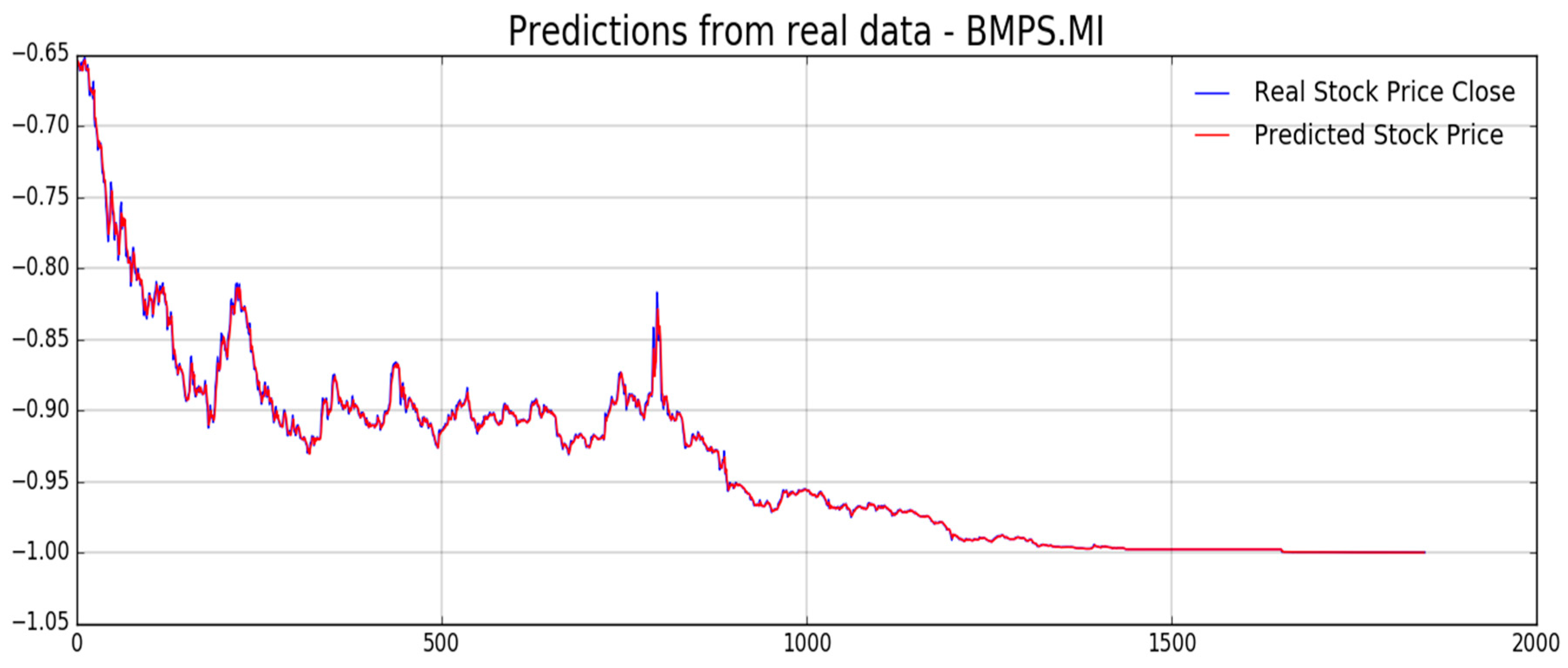
Figure 17, we report experimental results we obtained on forecasting analyzed stocks time series (close price) by means of second LSTM layer with prediction price correction based on the assumption of that share price formation satisfies Markov propriety. In order to show the advantages of the proposed Markov-based price prediction correction with respect to classical LSTM based prediction system, in
Figure 13 and
Figure 15 the authors show the same stock price prediction reported in
Figure 12 and
Figure 14, respectively, but without the described Markov-based correction. Moreover, we report such benchmark comparisons for showing the robustness and effectiveness of the proposed prediction pipeline.
As previously mentioned, one of the challenging target for the pipeline herein described is to provide an efficient mechanism for stock price prediction. The proposed method shows satisfactory results when doing shares price forecasting so that we decided to report such type of numerical metrics in order to exhibit the proper benchmark comparison of that capability.
The analyzed stock price prediction benchmark metrics are reported in
Table 1 and
Table 2. More in detail, in
Table 1, we report the average Root Mean Square Error (RMSE) for the single analyzed stock both in case of we apply the correction based on the assumption of price formation satisfies Markov propriety (RMSE
update) and without that correction, i.e., as it is performed by the trained LSTM only. From a simple analysis of the data reported in
Table 1, the assumption made by the author improves, significantly, the overall prediction performance of the proposed approach. In
Table 2, the authors report a further statistical comparisons index: The variance computed for the target stock price, as well as for the corresponding predicted ones (both with proposed Markov based correction “update” —and without that- “no update”), for each analyzed stock, in order to confirm how effective is our prediction model. As for
Table 1,
Table 2 reported statistic evaluations, confirm the robustness of the proposed approach. The benchmarks reported in
Table 1 and
Table 2 provide such statistic comparisons related to stock price forecasting. In order to improve that benchmark comparisons, we decided to evaluate the performance of the proposed approach by means of common robust indexes used in scientific literature for this purpose. The first comparison index we have used is described in Reference [
18] where the authors presented an innovative LSTM-based approach to predict financial indexes with comparable prediction errors. In Reference [
18], the authors showed an interesting benchmark comparison index suitable to evaluate the stock price prediction accuracy. In order to evaluate the proposed prediction algorithm of ups (LONG trend also knows as “Bullish”) and downs (SHORT trend also known as “Bearish”), the authors decided to calculate data accuracy by using the set of equation reported in Equations (16) and (17).
where
,
represents the real share price at time
i and
i + 1 respectively and, than,
represents the actual financial trend of the analyzed stock. We apply the same clustering as per Equation (16) to the set of predicted values. Obviously, the term
(1: if the predicted trend is correct 0: otherwise) represents an average benchmark metric of the predicted trends.
The accuracy reached by authors in Reference [
18] is in the range between 43% and 58% applied in the Shanghai Eastern market. The prediction accuracy of the proposed method is reported in
Table 3. With a benchmark DA index in the range 50% to 99% our method confirms the robustness and the efficiency on stock price prediction.
At the end, the authors provide a further robustness benchmarks usually used in the financial market, i.e., the si called drawdown. It is so defined in Reference [
19]: “A drawdown is the peak-to-trough decline during a specific recorded period of an investment, fund or commodity security. A drawdown is usually quoted as the percentage between the peak and the subsequent trough.” We performed a drawdown measure check of the proposed pipeline. The results are reported in
Table 4.
If we compare Maximum Drawdown results reported in
Table 4 with similar ones reported in a recent algorithm based on Machine Learning technique [
20], we easily understand that our proposed approach shows acceptable drawdown as it exposes almost 11 % of the total amount of investment which is a very promising result in the field of financial sustainable trading system [
20]. Finally, the results we have obtained in stock price prediction by means of the proposed pipeline confirms the robustness and the effectiveness of the approach are herein described, getting up the overall accuracy of the proposed prediction system based on the LSTM only. The benchmark comparison reported in
Table 1,
Table 2,
Table 3 and
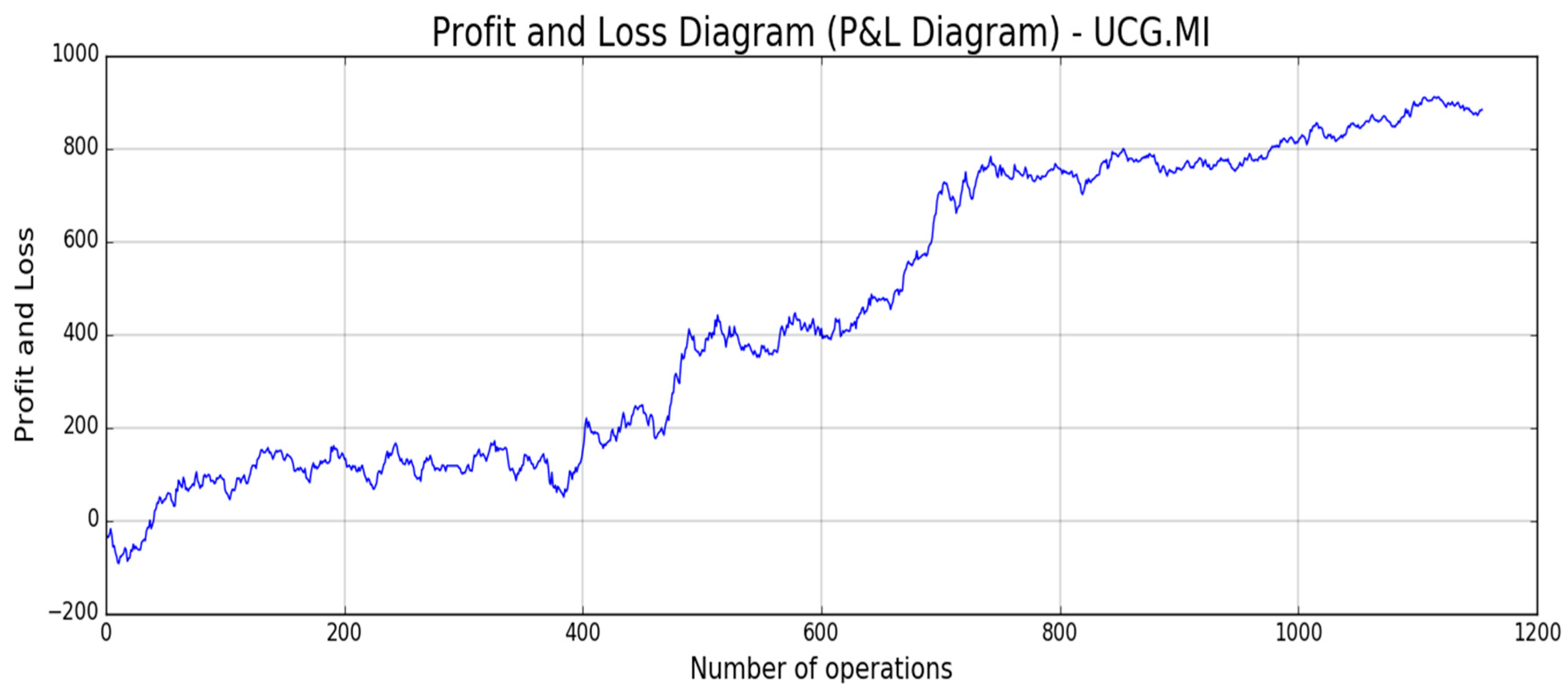
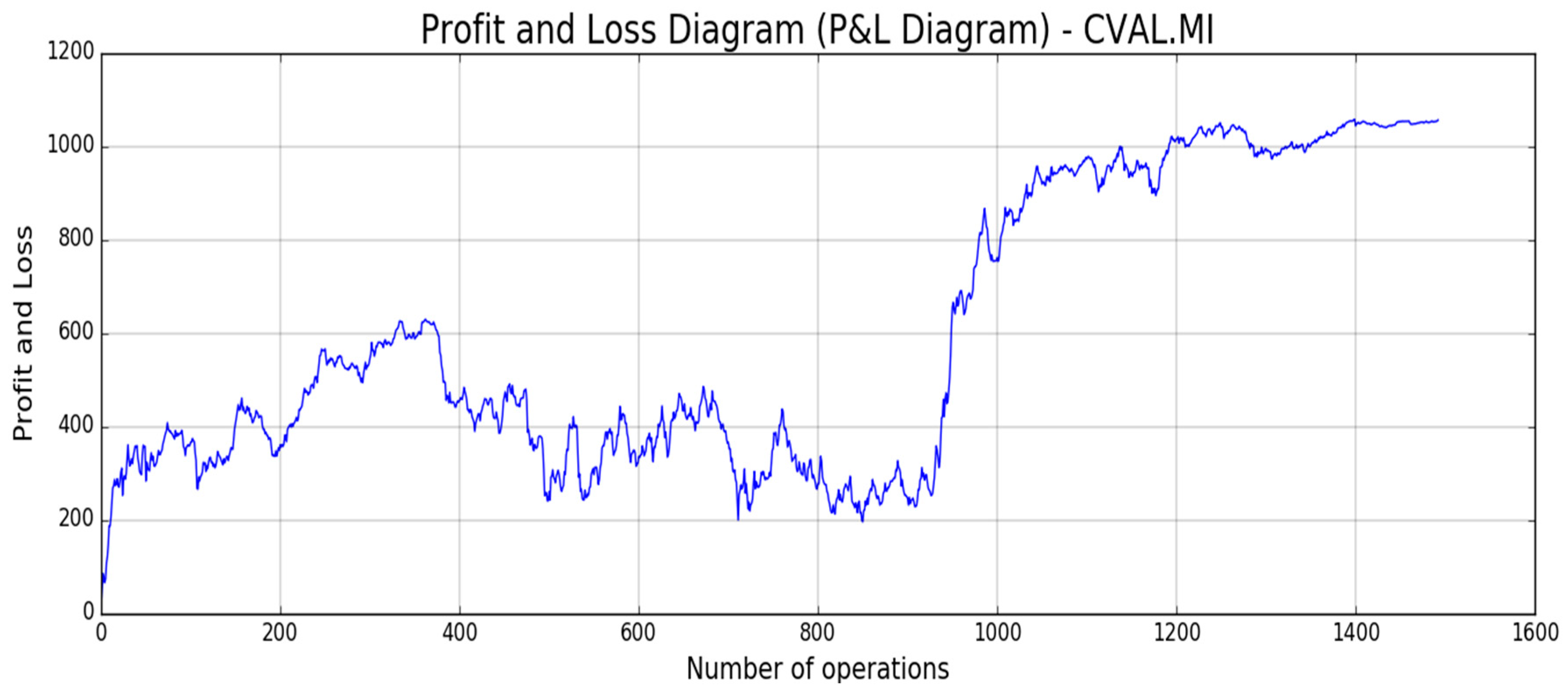
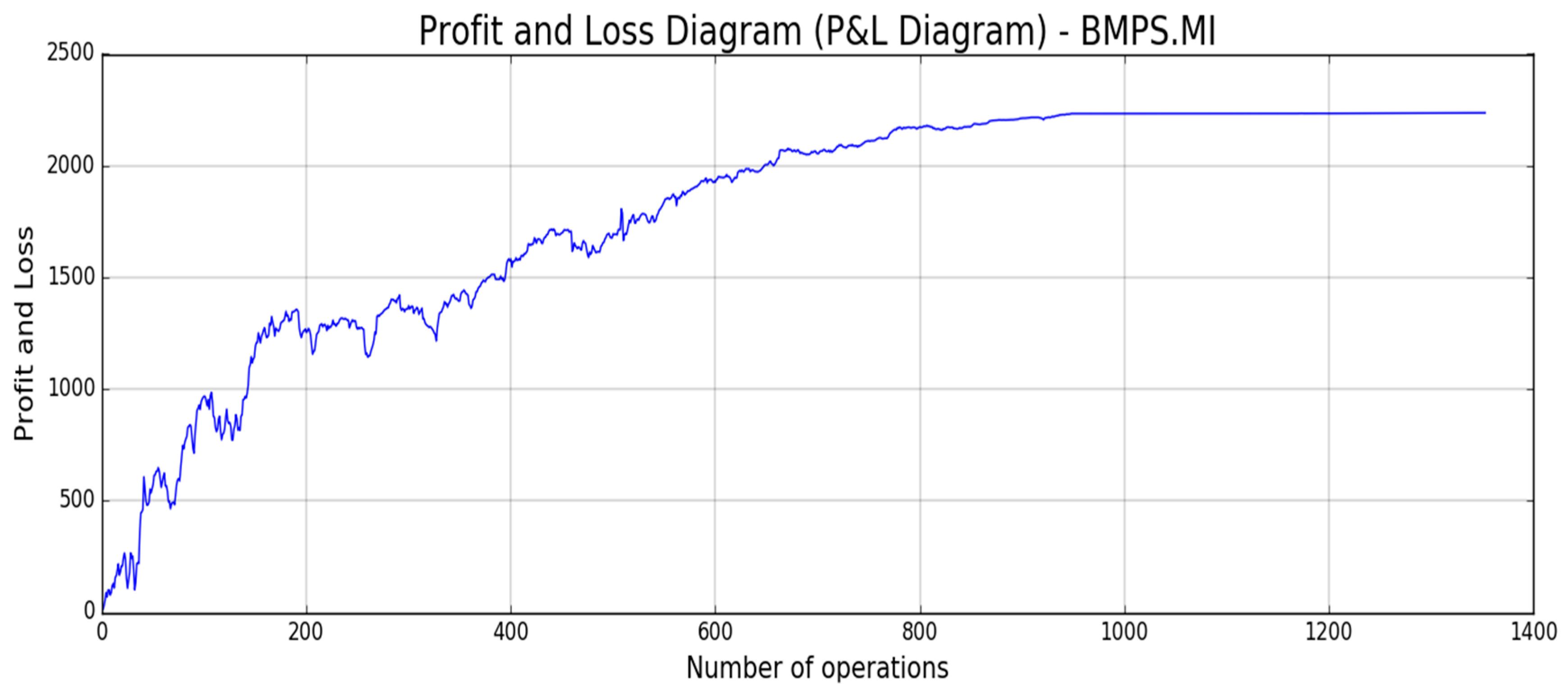
Table 4 confirms the mentioned advantages. Now, in order to validate the performance of the overall proposed system including the trading pipeline block, we have applied, as described in the previous section, our proposed pipeline for trading several stocks in the Milan Stocks Exchange Market. In
Figure 18,
Figure 19,
Figure 20,
Figure 21 and
Figure 22, the reported results of classical Profit and Loss Diagram (P&L) computed in EURO currency (y axes) are shown.
The above figures show a very promising P/L trend with an encouraging profit trend-line together with a contained drawdown as reported in
Table 4. Both results obtained for such different stocks confirm the robustness and the effectiveness of the proposed approach because it is able to find a good trade-off between profit and risk as the maximum drawdown is really sustainable for this type of investment.

