Finite Element Modellingand Simulations of Piezoelectric Actuators Responses with Uncertainty Quantification

Abstract

Piezoelectric structures are widely used in engineering designs including sensors, actuators, and energy-harvesting devices. In this paper, we present the development of a three-dimensional finite element model for simulations of piezoelectric actuators and quantification of their responses under uncertain parameter inputs. The implementation of the finite element model is based on standard nodal approach extended for piezoelectric materials using three-dimensional tetrahedral and hexahedral elements. To account for electrical-mechanical coupling in piezoelectric materials, an additional degree of freedom for electrical potential is added to each node in those elements together with their usual mechanical displacement unknowns. The development was validated with analytical and experimental data for a range of problems from a single-layer piezoelectric beam to multiple layer beams in unimorph and bimorph arrangement. A more detailed analysis is conducted for a unimorph composite plate actuator with different design parameters. Uncertainty quantification was also performed to evaluate the sensitivity of the responses of the piezoelectric composite plate with an uncertain input of material properties. This sheds light on understanding the variations in reported responses of the device; at the same time, providing extra confidence to the numerical model.

1. Introduction

Piezoelectric materials can be found in a wide variety of products from kitchen appliances to automobile industries and health care devices. The extensive use of piezoelectric materials in many engineering applications is due to its unique physical characteristics resulting from its specific material properties. Piezoelectric materials are crystalline materials in which mechanical and electrical states interact with each other. The mechanical and electrical states interact in a material with charged particles with no center of symmetry. Three types of microscopic level charge disorientation produce the macroscopic level polarization in a dielectric material, including electric and ionic polarization and dipole reorientation [1]. In the electronic polarization, the applied electric field deforms the electronic cloud, but in the case of ionic polarization, the applied electric field pushes the anion to the anode and the cations to the cathode. In the dipole reorientation, an applied electric field reorients the dipole directions in the separate domain of the material in one direction to polarize the material. The latter method is valid for the macroscopic non-polarized material consisting of many polarized volumes. A widely-used class of piezoelectric materials is a polycrystalline structure of lead zirconate titanate, Pb(Zr${}_x$Ti${}_{1-x}$)O${}_3$, also known as PZT which is a solid solution of two materials, lead titanate PbZrO${}_3$ and lead zirconate PbTiO${}_3$. The Zr and Ti ions in a lattice of an unpolarized PZT material are randomly distributed to neutralize the electrical polarity. The application of a high electric field at a temperature close to the Curie point aligns the Zr and Ti ions in lattices to polarize the materials. In another class of piezoelectric materials, molecular dipoles of polar polymers such as Polyvinylidene Fluoride (PVDF) are reoriented in one direction.

The ability of piezoelectric materials to generate electric potential from a mechanical strain and vice versa provides opportunities to use these materials as sensors or actuators found in many types of transducers. A sensor transforms mechanical energy to electrical output for monitoring purposes, and an actuator normally converts electrical energy to mechanical motions. The widely-discussed use of piezoelectric materials as sensors is found in the sonar (sound navigation and ranging) system, a sound-based navigation system, in which the electro-acoustic transducer converts the acoustic signals to the electrical signals. Ultrasound equipment in the medical industry uses the piezoelectric actuator to convert the electrical signal to mechanical vibration. A quartz wrist watch uses a piezoelectric actuator to convert electrical energy from a battery to mechanical vibration, which moves the second, minute, and hour arms of the watch. More recently, researchers have been exploring piezoelectric materials in their innovations such as heart rate monitors [2], piezoelectric-based toe-heaters for frostbite protection [3], and conversion of ocean wave energy to electrical energy [4]. Piezoelectric materials are also widely used in many droplet-on-demand applications including inkjet head printers, spraying devices, etc. For its wide ranging applications, understanding the characteristics of piezoelectric materials is essential in the process of the design and optimization of those devices.

Characterizing piezoelectric material behaviors is typically done through experiment with a specific design and prototype. Besides experimental characterization, there exist different analytical and numerical methods to model and analyze the responses and characteristics of piezoelectric material-based devices. Equivalent circuits [5], spring models [6], and thermal analogy [7] are analytical methods to model the simplified piezoelectric materials. For three-dimensional analysis, the finite element method has been a popular choice for modeling and simulations of piezoelectric material responses. Since the pioneering work of [8] on the application of the finite element method for piezoelectric materials, there have been numerous development of FEM tools to model piezoelectric structures ranging from solid three-dimensional elements to one- and two-dimensional elements such as beam, shell, and plates; including recent work on developing linear and quadratic shell elements [9,10]. In [11], a comprehensive review of the development of FEM was presented, classifying the number of different approaches based on element types, as well as the number of degrees of freedom. While the majority of solid three-dimensional FEM models focus on static and modal analysis of piezoelectric structures, there are fewer developments for unsteady analysis. This is even more desirable in Fluid-Structure Interaction (FSI) simulations when piezoelectric structure models are required to couple with flow models for analysis of FSI responses.

With this motivation, this paper presents an implementation of the Finite Element Method (FEM) to solve the piezoelectric problems and its applications to the design of piezoelectric actuators. In this work, the FEM implementation is based on the standard nodal approach extended for piezoelectric materials using three-dimensional tetrahedral and hexahedral elements. While hexahedral elements are mostly preferred in FEM analysis due to their superior accuracy and robustness, tetrahedral elements allow handling of complex geometries often encountered in practical applications. To account for electrical-mechanical coupling in piezoelectric materials, an additional degree of freedom for electrical potential is added to each node in those elements together with their standard displacement unknowns. The implementation of the piezoelectric model is based on an existing open source FEM code, OOFEM [12]. This presents the first significant contribution of the current work to the development of three-dimensional FEM as a general purpose analysis tool for piezoelectric materials.

For any numerical analysis, it is important to quantify errors associated with a model for quality assessment of its effectiveness and predictability. Apart from known errors present in the model, there are uncertainties from various sources including input parameters and material properties. There has been a great emphasis on verification and validation together with uncertainty quantification for numerical computations over the past few decades, including the pioneering work on the introduction of the Grid Convergence Index (GCI) [13] to a more general framework presented in [14,15]. Carrying out the error analysis and uncertainty quantification certainly provide confidence in the predictability of computational models. However, this process is cumbersome and time consuming, thus discouraging practitioners from adhering to those guidelines. In this work, a detailed framework of verification and validation was followed to access the convergence, as well as the accuracy of the proposed approach. Errors from uncertain parameters are also considered to establish bounds of prediction and investigate sources of discrepancy between numerical and experimental data. Uncertainties from different sources are identified, characterized, and quantified by propagating them through the model using the general framework proposed in [15].

The rest of the paper is organized as follows. In the next section, we present the mathematical foundation for the piezoelectric material modeling including a discussion on the finite element formulation for the dynamic piezoelectric problem. The numerical method is then validated with experimental data and analytical results for a number of problems ranging from a simple unimorph beam to three-layer plates. The last section of the paper presents an application of the developed method for analyzing the responses of piezoelectric actuators used in synthetic jet devices. It includes validation with experimental data, as well as quantification of uncertainties in material properties on response predictions.

2. Mathematical Formulations

2.1. Governing Equations for Piezoelectric Materials

The behavior of a piezoelectric material relating to the responses of the structure is strongly subjected to coupled electro-mechanical interactions. The dynamic response of a piezoelectric continuum of volume $\Omega$ bounded by surface $\Gamma =\partial \Omega$ is governed by momentum conservation equations and Gauss’s law in a dielectric as:

$$\begin{array}{c}\rho {\ddot{u}}_i={\sigma }_{ij,j}+\rho f_i^B,\hfill \end{array}$$

(1)

$$\begin{array}{c}{D}_{i,i}=0\hfill \end{array}$$

(2)

where ${\sigma }_{ij}$ and $D_i$ are the components of the Cauchy stress tensor and electric displacement vector. $\rho ,\mathrm{and}{f}_i^B$ are the density and body force, respectively. The displacement vector equation is the Gauss law written in the absence of free charges. The subscripts ${\left(\right)}_i$ and ${\left(\right)}_{ij}$ represent the $i^{\mathrm{th}}$ and ${(i,j)}^{\mathrm{th}}$ component of a vector and a matrix, respectively. The symbols $\ddot{\left(\right)},\mathrm{and}{\left(\right)}_{,i}$ represent $\frac{{\partial }^2\left(\right)}{\partial t^2}$ and $\frac{\partial \left(\right)}{\partial x_i}$, respectively. Typical boundary conditions are defined in

Table 1. Boundary conditions for the dynamic piezoelectric equations.

	Mechanical	Electrical
Natural Boundary Conditions	${\sigma }_{ij}{n}_j=f_i^b$ on $S_f$	$D_i{n}_i=q^s$ on $S_q$
Essential Boundary Conditions	$u_i=u_i^s$ on $S^u$	$\varphi ={\varphi }^s$ on $S_{\varphi }$

.

Constitutive equations for the coupled electromechanical problem are defined as:

$$\begin{array}{c}{\sigma }_{ij}=C_{ijkl}{\epsilon }_{kl}-e_{kij}{E}_k,\hfill \end{array}$$

(3)

$$\begin{array}{c}{D}_i=e^{ikl}{\epsilon }_{kl}+{ϵ}_{ik}{E}_k,\hfill \end{array}$$

(4)

where $C_{ijkl},{ϵ}_{kl}$, and $e_{kij}$ are elastic, dielectric material, and piezoelectric constants, respectively. The Cauchy strain tensor ${\epsilon }_{kl}$ is defined as:

$${\epsilon }_{kl}=\frac{1}{2}\left(u_{k,l}+u_{l,k}\right)$$

(5)

and the electric field vector component with an assumption of negligible magnetic effects is irrotational and can be represented in terms of electric potential, $\varphi$:

$${\epsilon }_{ijk}{E}_i{E}_j=0=>E_i=-{\varphi }_{,i},$$

(6)

where ${\epsilon }_{ijk}$ represents the Levi–Civita symbol.

2.2. Finite Element Discretization

According to the principle of virtual work for an arbitrary admissible variable of the displacement field $\delta u_i$ and the potential $\delta \varphi$ [11], the mechanical equilibrium can be written as:

$${\int }_{\Omega }\left({\sigma }_{ij,j}+\rho f_i^B-\rho {\ddot{u}}_i\right)\delta u_{i}d\Omega +{\int }_{\Omega }{D}_{i,i}\delta \varphi d\Omega =0.$$

(7)

Applying the divergence theorem and the boundary condition, Equation (7) can be re-written as:

$$-{\int }_{\Omega }{\sigma }_{ij}\delta {\epsilon }_{ij}d\Delta +{\int }_{\Omega }{D}_i\delta E_{i}d\Delta -{\int }_{\Omega }\rho {\ddot{u}}_i\delta u_{i}d\Omega +{\int }_{\Omega }\rho f_i^B\delta u_{i}d\Omega +{\int }_{\partial \Omega }{f}_i^b\delta u_{i}dS+{\int }_{\partial \Omega }{q}^s\delta \varphi dS=0$$

(8)

Applying constitutive equations with an assumption of zero free charge and zero induced potential, the variational Equation (8) can be written as:

$$\begin{array}{c}{\int }_{\Omega }\left(C_{ijkl}{\epsilon }_{kl}\delta {\epsilon }_{ij}-e_{ikl}{\epsilon }_{kl}\delta E_i\right)d\Omega +{\int }_{\Omega }\rho {\ddot{u}}_i\delta u_{i}d\Omega -{\int }_{\Omega }\rho f_i^B\delta u_{i}d\Omega \hfill \\ ={\int }_{\partial \Omega }{f}_i^b\delta u_{i}dS+{\int }_{\partial \Omega }{q}^s\delta \psi dS+{\int }_{\Omega }{e}_{ijk}{E}_k\delta {\epsilon }_{ij}d\Omega +{\int }_{\Omega }{ϵ}_{ik}{E}_k\left(\psi \right)\delta E_{i}d\Omega \hfill \end{array}$$

(9)

In a finite element model, the continuum domain is divided into a finite number of non-overlapping elements of simple geometrical shapes where the unknowns are calculated and stored at the nodes of elements. The displacement field $\left\{u\right\}$ and the electric potential $\left\{\phi \right\}$ over the element can be defined in terms of the nodal displacements $\left\{u_i\right\}$ and the nodal electric potentials $\left\{{\phi }_i\right\}$ using corresponding shape functions defined as $\left[N_u\right]$ and $\left[N_{\phi }\right]$, as in Equations (10) and (11), respectively.

$$\begin{array}{c}\left\{u\right\}=\left[N_u\right]\left\{u_i\right\}\hfill \end{array}$$

(10)

$$\begin{array}{c}\left\{\phi \right\}=\left[N_{\phi }\right]\left\{{\phi }_i\right\}\hfill \end{array}$$

(11)

The strain vector $\left\{\epsilon \right\}$ and the electric field $\left\{E\right\}$ are related to the displacement field $\left\{u\right\}$ and the electric potential $\left\{\phi \right\}$ using Equations (12) and (13), respectively:

$$\begin{array}{c}\left\{\epsilon \right\}=\left[\mathrm{D}\right]\left\{u\right\}\hfill \end{array}$$

(12)

$$\begin{array}{c}\left\{E\right\}=-▽\phi .\hfill \end{array}$$

(13)

Here, $\left[\mathrm{D}\right]$ is the derivation operator defined as:

$$\left[\mathrm{D}\right]={\left[\begin{array}{cccccc}\frac{\partial }{\partial x}& 0& 0& 0& \frac{\partial }{\partial z}& \frac{\partial }{\partial y}\\ 0& \frac{\partial }{\partial y}& 0& \frac{\partial }{\partial z}& 0& \frac{\partial }{\partial x}\\ 0& 0& \frac{\partial }{\partial z}& \frac{\partial }{\partial y}& \frac{\partial }{\partial x}& 0\end{array}\right]}^T,$$

(14)

and ▽ is the gradient operator. Substituting the values of $\left\{u\right\}$ and $\phi$ in the above equations, the strain and electrical field can be expressed in relation to the displacement nodal values $\left\{u_i\right\}$ and the potential nodal values $\left\{{\phi }_i\right\}$ as:

$$\begin{array}{c}\left\{\epsilon \right\}=\left[{\mathrm{B}}_u\right]\left\{u_i\right\}\hfill \end{array}$$

(15)

$$\begin{array}{c}\left\{E\right\}=\left[{\mathrm{B}}_{\phi }\right]\left\{{\phi }_i\right\},\hfill \end{array}$$

(16)

where $\left[{\mathrm{B}}_u\right]=\left[\mathrm{D}\right]\left[N_u\right]$ and $\left[{\mathrm{B}}_{\phi }\right]=-▽\left[N_{\phi }\right]$.

Substituting Equations (15) and (16) for the strain and the electric field into the variational principles (9), we obtain the coupled electromechanical formulation for the piezoelectric material written in discrete matrix form as:

$$\left[\begin{array}{cc}\left[M\right]& 0\\ 0& 0\end{array}\right]\left[\begin{array}{c}{\ddot{u}}_i\\ {\ddot{\varphi }}_i\end{array}\right]+\left[\begin{array}{cc}\left[K_{uu}\right]& \left[K_{u\varphi }\right]\\ {}_{\varphi u}]& \left[K_{\varphi \varphi }\right]\end{array}\right]\left[\begin{array}{c}{u}_i\\ {\varphi }_i\end{array}\right]=\left[\begin{array}{c}{f}_i\\ g_i.\end{array}\right]$$

(17)

Here, $\left[M\right]$, $\left[K_{uu}\right]$, $\left[K_{\phi u}\right]$, $\left[K_{\phi \phi }\right]$, $\left\{f_i\right\}$, $\left\{g_i\right\}$ are defined as:

$$\begin{array}{cc}\left[M\right]={\int }_{\Omega }\rho {\left[N_u\right]}^T\left[N_u\right]d\Omega ;\hfill & \hfill \left[K_{uu}\right]={\int }_{\Omega }{\left[{\mathrm{B}}_u\right]}^T\left[C^E\right]\left[{\mathrm{B}}_u\right]d\Omega ,\\ \left[K_{\phi u}\right]={\int }_{\Omega }{\left[{\mathrm{B}}_{\phi }\right]}^T{\left[e\right]}^T\left[{\mathrm{B}}_u\right]d\Omega ={\left[K_{u\phi }\right]}^T;\hfill & \hfill \left[K_{\phi \phi }\right]={\int }_{\Omega }{\left[{\mathrm{B}}_{\phi }\right]}^T\left[ϵ\right]\left[{\mathrm{B}}_{\phi }\right]d\Omega ,\\ \left\{f_i\right\}={\int }_{\Omega }\rho {\left[N_u\right]}^T\left\{f^B\right\}d\Omega +{\int }_{\partial \Omega }{\left[N_u\right]}^T\left\{f_b\right\}d\Omega ;\hfill & \hfill \left\{g_i\right\}={\int }_{\partial \Omega }{\left[N_{\phi }\right]}^T{q}^{s}dS.\end{array}$$

The discrete coupled Equation (17) can be implemented in any standard finite element packages. In a typical finite element implementation, problems are defined in a specific domain with a required number of Degrees of Freedom (DOFs). In this work, a domain (3dpiezo) was developed to solve for piezoelectro-mechanical coupled problems with 4-DOFs (u-, v-, w-displacement and voltage (V)). The linear piezoelectric hexahedral and tetrahedral elements were implemented in the open source finite element framework, OOFEM [12]. Figure 1 shows the node numbers of the element, and each node of the element has 4-DOFs. In this implementation, the global mass matrix, stiffness matrix, and force matrix are computed and assembled from the elemental mass matrix, stiffness matrix, and the right-hand side of the Equation (17) for each individual elements with the additional degree of freedom of electrical potential at each node. Appropriate boundary conditions for electro-mechanical coupling were also implemented in OOFEM for different types of loading. This developed model was applied and validated for a number of problems shown in the section about verification and validation.

2.3. Error and Uncertainty Quantification

When using numerical models for the prediction of structure responses, it is important to understand errors associated with the prediction, as well as any uncertainty arising from the process. Among different types of errors and uncertainties associated with computational modeling and simulations [14], three typical types of inaccuracy are considered in this work, namely discretization errors (${ϵ}_h$), input errors (${ϵ}_i$), and surrogate model errors (${ϵ}_s$):

$${ϵ}_{num}={ϵ}_h+{ϵ}_i+{ϵ}_s.$$

(18)

Discretization errors ${ϵ}_h$ are deterministic and classified as acknowledged errors resulting from errors due to numerical schemes used to discretize the governing equations. Generally, the discretization error can be approximated as proportional to some measure of grid resolution h,

$${ϵ}_h=f\left(h\right)-f_{true}\approx C{h}^p,$$

(19)

where f is a general quantity of interest and p is normally referred to as grid convergence order. In practice, the convergence order can be determined from solutions on grids with a successive refinement ratio of r as,

$$p=log\left(\frac{f\left(h_3\right)-f\left(h_2\right)}{f\left(h_2\right)-f\left(f_1\right)}\right)/log\left(r\right).$$

(20)

The discretization error can then be estimated as asymptotic convergence of error using Richardson extrapolation as:

$${ϵ}_h=f_{h=0}-f\left(h_1\right)\approx \frac{f\left(h_1\right)-f\left(h_2\right)}{r^p-1}.$$

(21)

This requires additional evaluation of the quantities of interest at a grid finer than the current grid to estimate the discretization error.

Ideally, inputs to computational models should be the same as in actual physical systems. However, due to a lack of knowledge, equipment errors, or variability in measurement techniques, there are discrepancies in input parameters between physical and numerical models. This uncertainty, such as the material properties and the geometrical dimensions of the apparatus, potentially introduces errors to numerical predictions. The input errors ${ϵ}_i$ are normally stochastic and represented as random variables with a normal distribution of a zero mean and a constant bias. Assume that the input $\mathit{\xi }$ to a model with expected output function f is random with a suitable probability distribution $p\left(\mathit{\xi }\right)$. The input error to a computational model can be accounted for by propagating its randomness through the model to the final output. The statistical properties of output function f such as the mean ${\mu }_f$ and the variance ${\sigma }_f^2$ are defined as:

$${\mu }_f=\int f\left(\mathbf{\xi }\right)p\left(\mathbf{\xi }\right)d\xi ,{\sigma }_f^2=\int {(f\left(\mathbf{\xi }\right)-{\mu }_f)}^{2}p\left(\mathbf{\xi }\right)d\xi .$$

(22)

To quantify the uncertainty propagation through computational models, there are various techniques dependent on the types of uncertainties, as well as a representation of output uncertainty [15]. For aleatory uncertainties presented in this work, the Latin Hypercube Sampling (LHS) approach and stochastic expansion (polynomial chaos expansion) technique are applied for characterizing the propagation of uncertainties through the developed FEM. Given a probability distribution of input, a sampling-based approach will evaluate the output on the quantities of interest at various sample points one-by-one to build a discrete representation of output responses. For traditional random sampling, also known as the Monte Carlo approach, it requires a large number of samples to determine the output distribution accurately. In the LHS approach, each input variable is divided into N-bins of equal probability, and a sample point is uniformly determined from a unique bin for each variable, thus avoiding clustering of samples. LHS requires less sample points as compared to random sampling for the same accuracy. Alternatively, to alleviate the problems of large sample sizes, a response function can be built from a limited number of sample points using polynomial chaos expansion. This approximation is considered as a surrogate model to the more expensive computational model and allows evaluation of a much larger number of output functions for a more accurate distribution. However, there is an error associated with this surrogate model that needs to be taken into account during the uncertainty quantification process. Consider a PCEof output function f using Hermite polynomial basis functions $\mathit{\varphi }=\{{\varphi }_0(.),{\varphi }_1(.),\cdots ,{\varphi }_n(.)\}$,

$$f_{PCE}\left(\mathbf{\xi }\right)\approx \sum _{j=0}^n{\lambda }_j{\varphi }_j$$

(23)

It has been shown [16] that errors for PCE surrogate models built from m training data points $(f_i,{\mathit{\xi }}_i),i=1,2,\cdots ,m$ follow a normal distribution with zero mean and variance given as:

$$Var\left[{ϵ}_s\right]\approx s^2+s^2\mathbf{\varphi }{\left(\mathbf{\xi }\right)}^T{\left({\mathsf{\Lambda }}^T\mathsf{\Lambda }\right)}^{-1}\mathbf{\varphi }\left(\mathbf{\xi }\right),$$

(24)

where $\mathsf{\Lambda }=\{\mathit{\varphi }\left({\mathit{\xi }}_1\right),\cdots ,\mathit{\varphi }\left({\mathit{\xi }}_m\right)\}$ and $s^2=\frac{1}{m-n}{\sum }_{i=1}^m\left[f_i-f_{PCE}\left({\mathit{\xi }}_i\right)\right]$. One can refer to the earlier work [15] and the references cited therein for more details about the LHS and PCE approaches.

3. Verification and Validation

In this section, the developed FEM solver is applied to a number of test case ranging from a simple beam to more complex piezoelectric structures used in the design of actuators. The results of the solver are validated with experimental and analytical data to establish its accuracy, as well as the convergence rate.

3.1. Single-Layer Piezoelectric Beam

A single-layer piezoelectric beam with PZT-5Hmaterial was used to validate the solvers for static responses. The material properties of PZT-5H are specified in

Table 2. Material properties of PZT-5H.

$\mathit{\rho }=7500$	(kg/m${}^3$)
$\left[c\right]=\left[\begin{array}{cccccc}12.6& 7.95& 8.41& 0& 0& 0\\ 7.95& 12.6& 8.41& 0& 0& 0\\ 8.41& 8.41& 11.7& 0& 0& 0\\ 0& 0& 0& 2.3& 0& 0\\ 0& 0& 0& 0& 2.3& 0\\ 0& 0& 0& 0& 0& 2.325\end{array}\right]$	× 10${}^{10}$ (Pa)
$\left[\epsilon \right]=\left[\begin{array}{ccc}1700{\epsilon }_0& 0& 0\\ 0& 1700{\epsilon }_0& 0\\ 0& 0& 1470{\epsilon }_0\end{array}\right]$
$\left[e\right]=\left[\begin{array}{cccccc}0& 0& 0& 0& 17& 0\\ 0& 0& 0& 17& 0& 0\\ -6.5& -6.5& 23.3& 0& 0& 0\end{array}\right]$	(Cb/m${}^2$)

and used throughout the current work. Figure 2 shows the schematic of the case setup with detailed dimensions. The case represents a multilayered design of a piezoelectric actuator frequently used in engineering applications.

There are two main actuation modes for a multilayered design dependent on the orientation of the poling direction and electrical field. For in-plane mode, tensile deformations are achieved by applying the voltage in the poling direction. When the electric field is parallel to the poling direction, the in-plane and the thickness deformation can be analytically obtained as [1]:

$$\mathit{u}=(u_x,u_y,u_z)=\left(\frac{d_{31}\varphi L}{h},\frac{d_{32}\varphi w}{h},d_{33}\varphi \right).$$

(25)

Alternatively, the laminar beam can be actuated in shear mode where the electrical field is applied perpendicular to the poling direction. In this case, the coupling coefficient $d_{15}$ controlled the design. The analytical solution of bending displacement is given [1] as:

$$\Delta =\frac{L{d}_{15}\varphi }{h}.$$

(26)

Tensile and shear deformation cases were analyzed with the developed FEM solvers using two different element types. Figure 3 shows the displacement contours of the beam under in-plane and shear mode of displacement. In this case, an electrical field was applied in the thickness z-direction, while the poling direction was changed from the z-direction for in-plane mode to the x-direction for shear mode.

Table 3. Displacement prediction from the FEM solver with different types of elements (tetrahedral and hexahedral) for a single-layer PZT beam under tensile and shear load.

			Tensile			Shear
	Δ (mm)	${\mathit{N}}_{\mathit{e}}$	${\mathit{u}}_{\mathit{x}}$	${\mathit{u}}_{\mathit{y}}$	${\mathit{u}}_{\mathit{z}}$	|$\mathit{u}$|
Tet	1	780	1.37 × 10${}^{-7}$	6.85 × 10${}^{-8}$	5.93 × 10${}^{-8}$	3.900 × 10${}^{-7}$
-	0.2	49,960	1.37 × 10${}^{-7}$	6.85 × 10${}^{-8}$	5.93 × 10${}^{-8}$	3.900 × 10${}^{-7}$
Hex	1	100	1.37 × 10${}^{-7}$	6.85 × 10${}^{-8}$	5.93 × 10${}^{-8}$	3.696 × 10${}^{-7}$
-	0.2	10,000	1.37 × 10${}^{-7}$	6.85 × 10${}^{-8}$	5.93 × 10${}^{-8}$	3.696 × 10${}^{-7}$
Analytical	-	-	1.37 × 10${}^{-7}$	6.85 × 10${}^{-8}$	5.93 × 10${}^{-8}$	3.695 × 10${}^{-7}$

summarizes the comparison of the prediction from the model on the displacement of the PZT beam under tensile and shear mode with reference to the analytical solution. It can be seen that the FEM model provided exact displacement compared to the analytical response on a very coarse grid for the tensile case with both a tetrahedral and hexahedral element. For the bending case, tetrahedral elements resulted in a larger deflection compared to analytical displacement; the error was about $5.4\%$, as shown in Table 3. This simple test demonstrated the well-known superiority of hexahedral elements compared with tetrahedral ones in bending modes. In subsequent examples, hexahedral elements were used for most of the cases, unless otherwise specified.

3.2. Bimorph Piezoelectric Beam

A widely-used bimorph case with opposite polarities at the different layers, commonly used to validate the shell and plate elements [1], was used to validate the solver for a very high aspect ratio of the beam length to the beam height scenario. The bimorph setup can be used as a micro-actuator or a micro-sensor. Figure 4 shows the schematic of the bimorph piezoelectric beam consisting of two geometrically-similar uniaxial piezoelectric layers with opposite polarity. These layers are stacked together to obtain the opposite strain in layers, resulting in bending when voltage is applied across the thickness.

Opposite polarity of the beams with the voltage across the thickness generates moment to bendthe bimorph beam. An analytical solution of the bimorph beam deflection is given as Equation (27) using the classical theory of beams [1].

$$z\left(x\right)=\frac{3}{2}\frac{d_{31}\varphi }{h^2}{x}^2$$

(27)

The material used in the bimorph beam simulation was PZT-5H, and the properties of the material are listed in Table 2.

To validate the solver for simulations of an actuator, $\varphi =100\mathrm{V}$ was applied across the thickness of the beam with $L=100\mathrm{mm}$, $b=5\mathrm{mm}$, and $h=1\mathrm{mm}$. The three-dimensional hexahedral piezoelectric element was used to simulate the beam with the finite element methods, and the computed static beam deflection was compared with the analytical results, as shown in Figure 5a. Figure 5b plots the reducing error with the increasing number of elements in the simulations. The error was measured as the difference of computed deflection with analytical prediction using beam theory. It can be seen that a second-order convergence was observed in this case, as expected for FEM analysis.

3.3. Three-Layer Actuator Beams

The solver is further validated with a three-layer beam case [17] with two piezoelectric beams attached to the non-piezoelectric beam, as shown in Figure 6. The poling directions of the piezoelectric beams were parallel to the z-axis, and the voltage $v=100$ V was applied at the free sides in the z-direction of the three-layer actuator beam setup. L is the length of the non-piezoelectric beam, and the piezoelectric layers have a length of $l=x_1-x_2$, where $x_1=\frac{L}{12}$ and $x_2=\frac{5L}{12}$.

The analytical solution of the problem is given [17] as:

$$\begin{array}{c}\hfill z\left(x\right)=\frac{-3d_{31}{E}_p(t_b+t_b)}{E_b{t}_b^3-3E_p{t}_b(3t_b^2+6t_p{t}_b+2t_p^2)}\left\{H[x-x_1]{(x-x_1)}^2-H[x-x_2]{(x-x_2)}^2\right\}v,\end{array}$$

(28)

where ($t_p$, $t_b$) and ($E_p$, $E_b$) are the thickness and Young’s modulus of the piezoelectric layer and the non-piezoelectric beams, respectively. Here, $x\le L$ is the location at which the vertical deflection $z\left(x\right)$ of the cantilever converter is calculated. The geometrical and material properties used in the numerical simulations were $E_p=7.7$ × 10${}^{10}$ $\mathrm{N}/{\mathrm{m}}^2$, $E_b=2.0$ × 10${}^{11}$ $\mathrm{N}/{\mathrm{m}}^2$; Poisson’s ratio ${\nu }_p=0.3$, ${\nu }_b=0.33$; density ${\rho }_p=7700\mathrm{kg}/{\mathrm{m}}^3$, ${\rho }_b=7860\mathrm{kg}/{\mathrm{m}}^3$. The piezoelectric strain coefficient matrix d is defined in

Table 4. Piezoelectric coefficients for the piezo layer in the three-layer beam case.

$\left[d\right]=\left[\begin{array}{cccccc}0& 0& 0& 0& 3.27& 0\\ 0& 0& 0& 3.27& 0& 0\\ -1.28& -1.28& 3.28& 0& 0& 0\end{array}\right]$ × 10${}^{-10}$

(m/V)

.

Figure 7a shows the deflection of the beam with different numbers of elements, while Figure 7b plots the reducing error with the increasing number of elements in the simulations. It is clearly seen that the deflection profile converged to analytical results with mesh refinement. However, the rate of convergence was not second order, as in the previous examples.

4. Uncertainty Quantification of the Piezoelectric Composite Plate Actuator’s Response

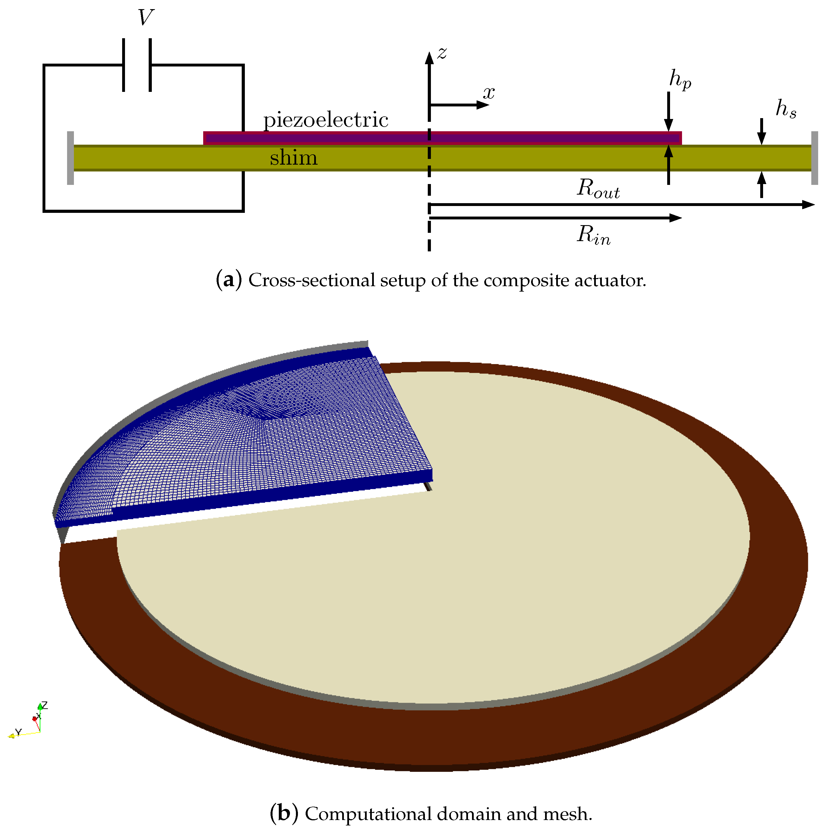
Composite plate piezoelectric actuators are found in many electroacoustic devices, including microphones, micropumps, synthetic jets, etc. The actuator comprises a circular plate of piezoelectric material bonded with a metallic material plate, and actuation is achieved by applying electrical potential on an electrode attached to the piezoelectric layer. Figure 8a shows a typical setup of a composite piezoelectric unimorph actuator (APC 850) [18,19]. In this current setup, a piezoelectric plate of thickness $h_p$ and radius $R_{in}$ was bonded with a shim disc of thickness $h_s$ and radius $R_{out}$. The shim plate was fully clamped, and the material properties of APC 850 were taken from

Table 5. Dimensions and material properties of the APC 850 actuator extracted from [18].

Geometric Properties
Outer radius	$R_{out}$ (mm)	11.7
Radius of piezoelectric	$R_{in}$ (mm)	10.0
Radius of silver	$R_s$ (mm)	9.2
Thickness of shim	$h_s$ (mm)	0.221
Thickness of piezoelectric	$h_p$ (mm)	0.234
Thickness of silver	h (mm)	0.015
Material Properties
Elastic modulus of shim	$E_s$ (GPa)	90
Poisson’s ratio of shim	${\lambda }_s$ (-)	0.32
Density of shim	${\rho }_s$ (kg/m${}^3$)	8700
Elastic modulus of piezoelectric	$E_p$ (GPa)	63
Poisson’s ratio of piezoelectric	${\lambda }_p$ (-)	0.31
Density of piezoelectric	${\rho }_p$ (kg/m${}^3$)	7700
Electrical Properties
Relative dielectric constant	${ϵ}_r$ (-)	1750
Piezoelectric constant	$d_{31}$ (m/V)	$-175\times {10}^{-12}$

extracted from [18,20]. The computational domain was taken as one quarter of the composite plate in which symmetric conditions were applied at the cut planes. Figure 8b shows a block-structured mesh of the computational domain where it is characterized by $N_1$ number of points in the radial and azimuthal directions of blocks on the piezoelectric plate, $N_2$ number of points (radial and azimuthal) on the blocks of the shim, and $N_3$ number of layers extruded in the thickness direction for each plate.

4.1. Characterization and Comparison of Actuator Responses

It is important to characterize the responses of the actuator for design purposes. Prasad et al. [18,19] presented several models for response predictions of unimorph actuators including a lumped element model and the analytical model based on plate element theory. 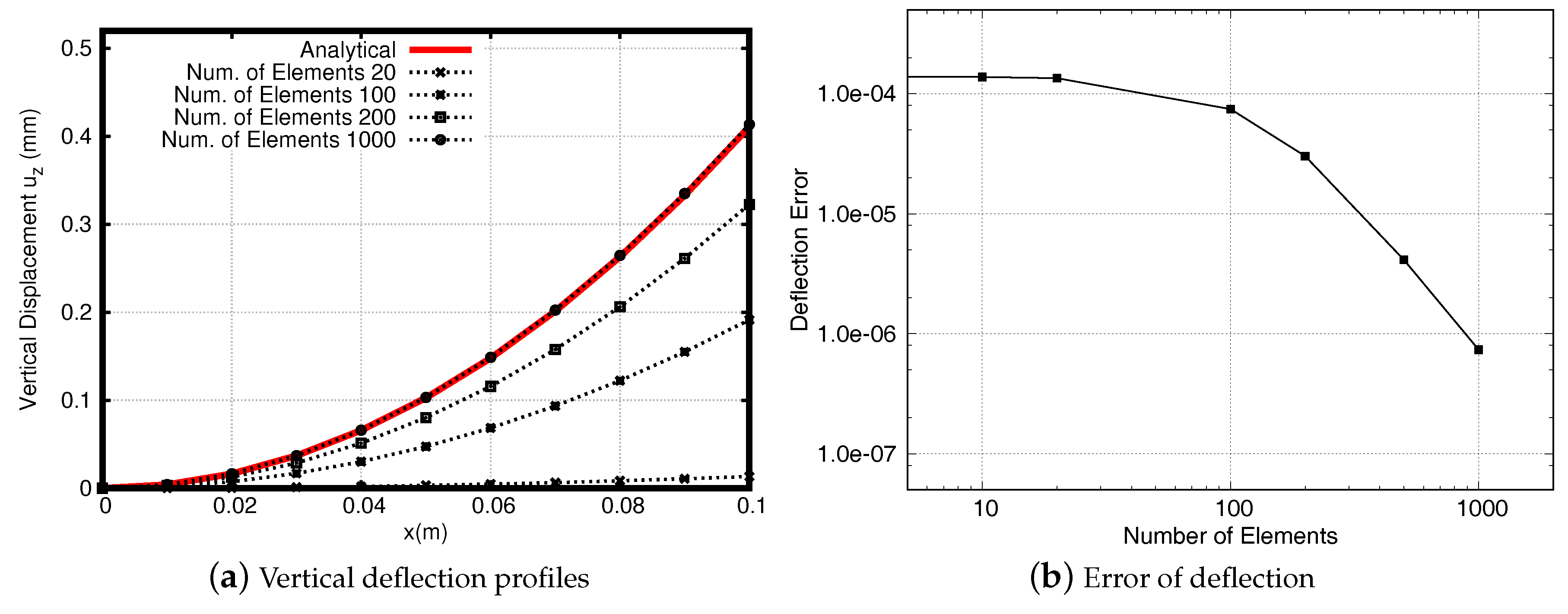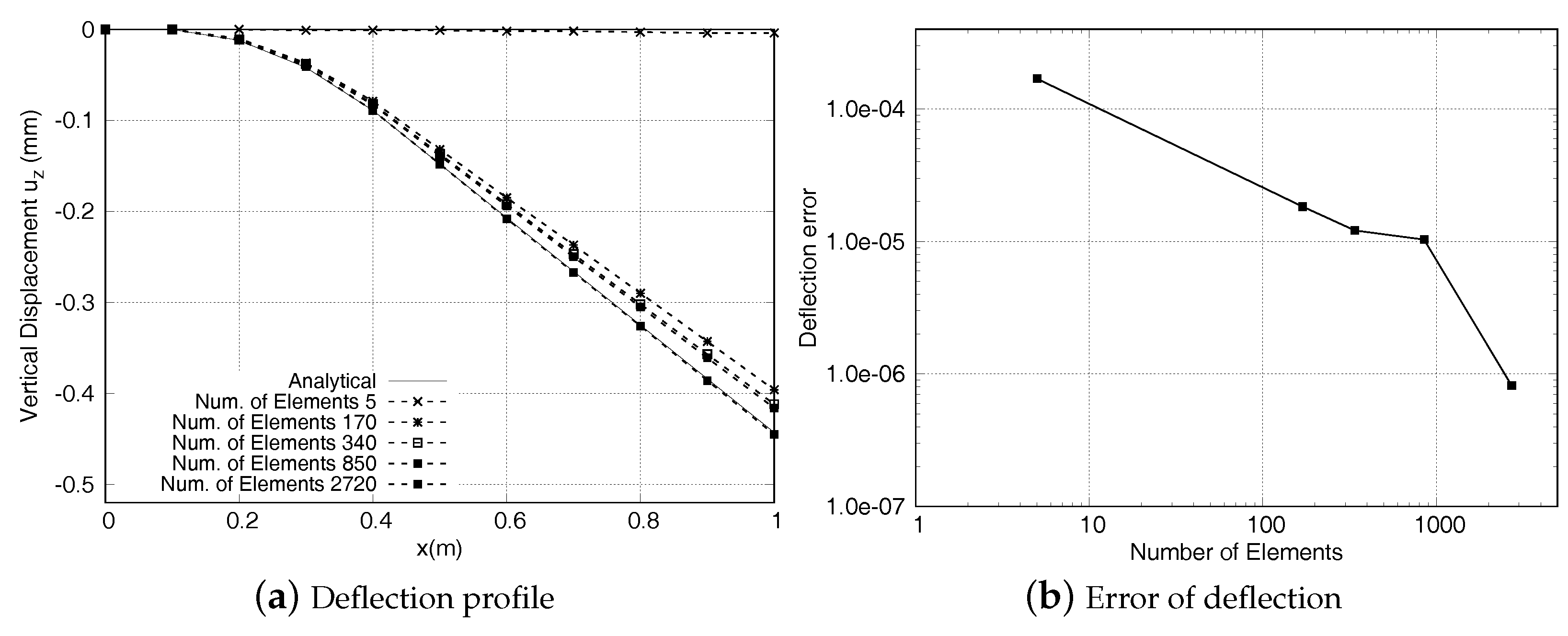It is known that the maximum deflection of the actuator is dependent on the plate thickness ratio ($h_p/h_s$), radius ($R_{out}/R_{in}$), and material properties. Here, FEM was applied for static analysis of the actuator under voltage load of 5 V. A mesh sensitivity study is shown in Figure 9 for the radial deflection profile with clear convergence of numerical prediction when the mesh is refined.

Table 6. Mesh sensitivity study and convergence index for the unimorph actuator. GCI, Grid Convergence Index.

Grid	${\mathit{N}}_{\mathit{r}1}$	${\mathit{N}}_{\mathit{r}2}$	${\mathit{N}}_{\mathit{h}}$	${\mathit{u}}_{\mathit{z},\mathit{max}}$ ($\mathsf{\mu }$m/V)	GCI (%)
G1	40	10	4	0.08809	-
G2	60	20	6	0.09167	2.89
G3	80	30	8	0.09653	6.03
G4	100	40	10	0.09918	4.44
Asymptotic	-	-	-	0.10499	-

shows the convergence index with the mesh refinement. At the finest mesh, the maximum displacement was about $4.44\%$ away from the asymptotic value of the predicted displacement. The order of convergence estimated according to Equation (20) is:

$$p=log\left(\frac{u_{z,max}^{G3}-u_{z,max}^{G2}}{u_{z,max}^{G2}-u_{z,max}^{G1}}\right)/log\left(r\right)=2.016,$$

(29)

which is approximately the same as the theoretical convergence order of the FEM formulation. It can be seen that the asymptotic FEM result was larger compared with the experimental and analytical data in [18]. As explained in [18], the difference could be due to the fact that the silver electrode layer, as well as the glue between plates were not modeled in the FEM analysis. Looking further into the experimental data, it was found that the device (APC 850) used in a later work by the same author [19] showed a slightly different response experimentally and analytically.

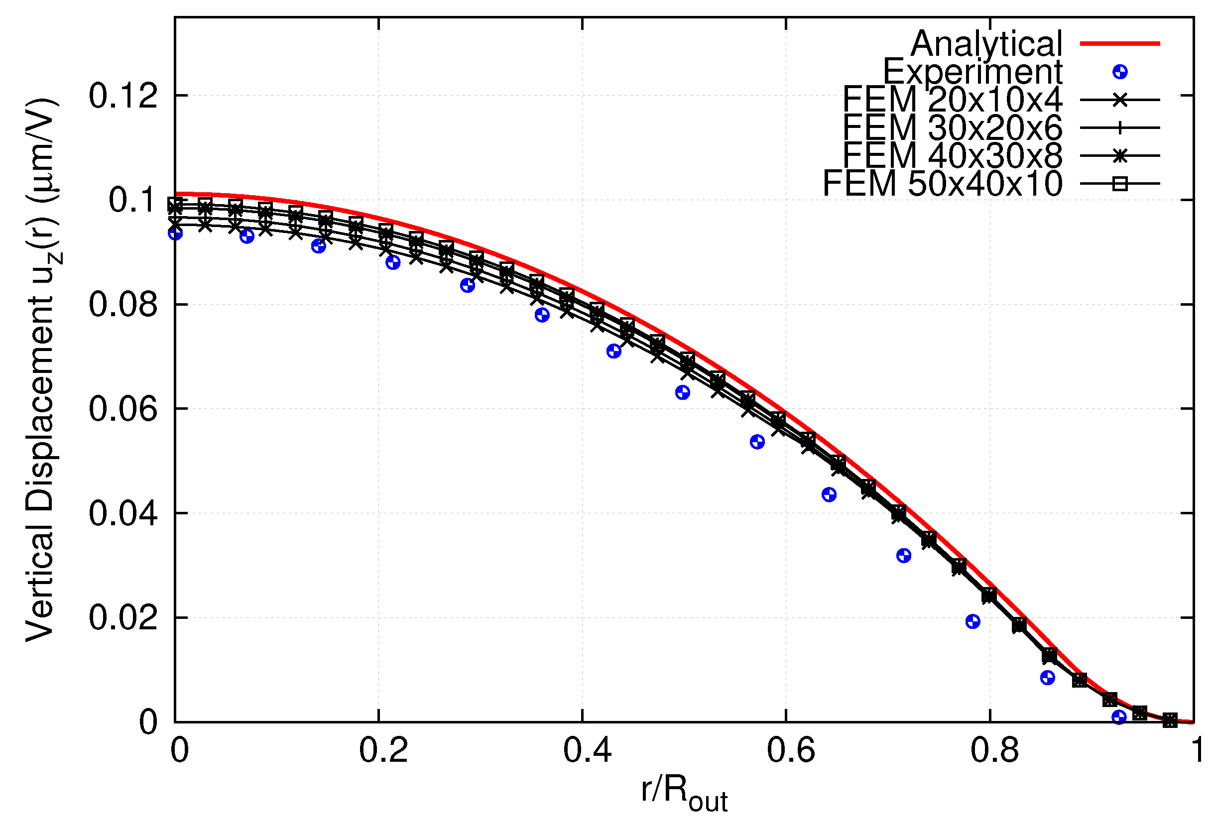
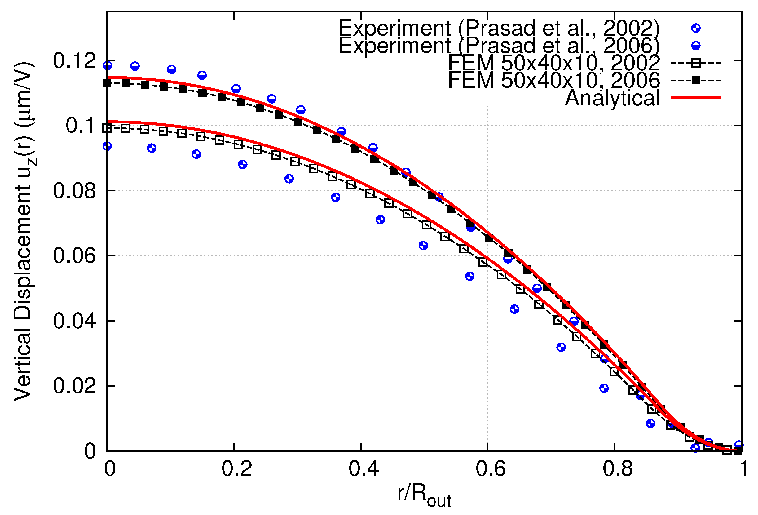
Figure 10 shows experimental data from two different references for the same reported device. It can be seen that the difference on deflection of the disc was very large between the two configurations where maximum deflection at the center of the disc increased $24\%$ from 0.0937 $\mathsf{\mu }$m–0.1184 $\mathsf{\mu }$m per unit applied voltage. For these two configurations, the only significant difference in the setup was the thickness of the shim layers. The current FEM results showed an increase in response amplitude with reducing shim thickness, as observed in the experiment. 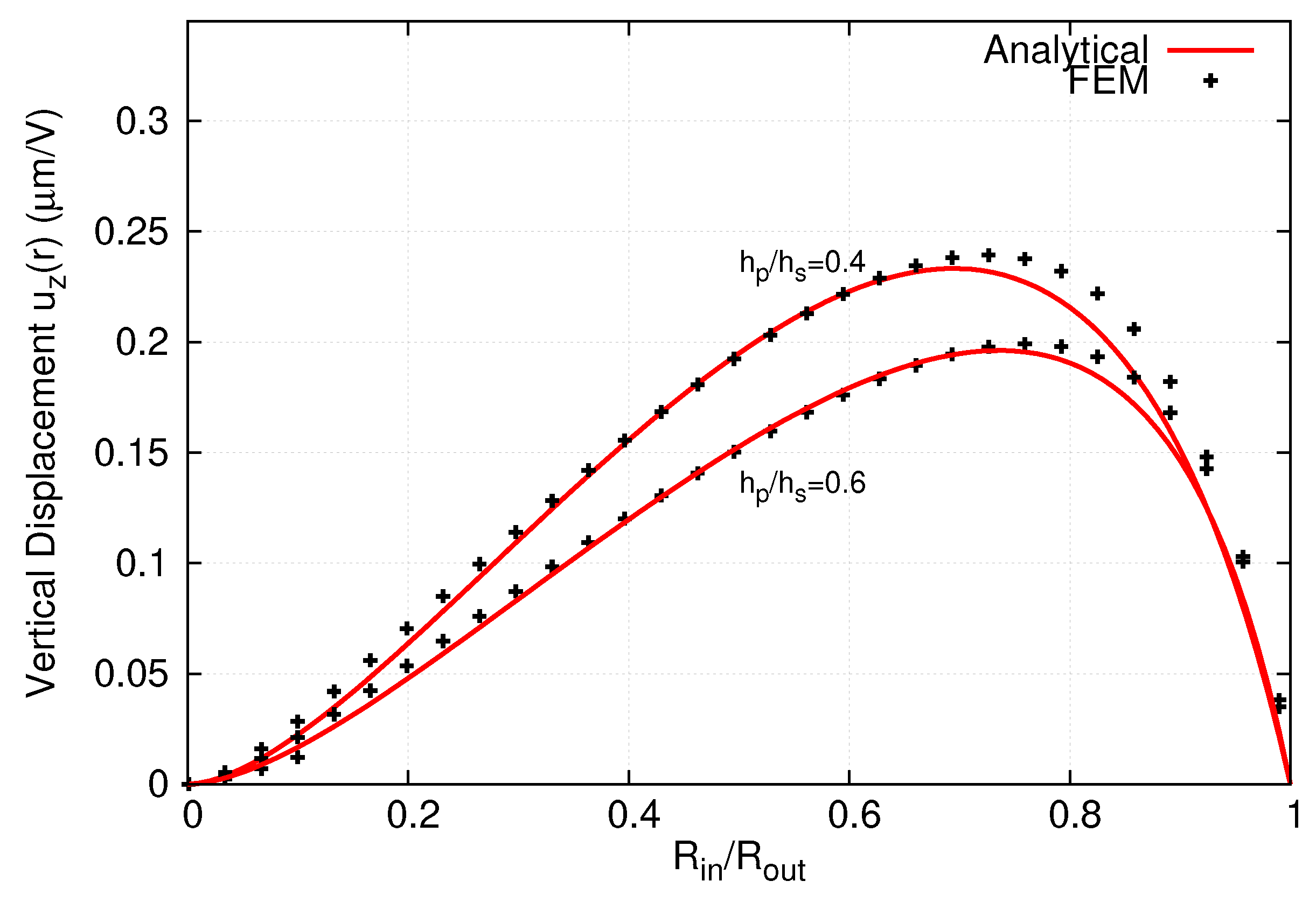This is further illustrated in Figure 11, where maximum displacements are shown with changing of the shim and plate thickness ratio in the variation of their radius. The maximum displacement also increased with increasing radius ratio. This behavior could help in explaining the discrepancies between current FEM analysis with experimental data. However, it led to uncertainties in the analysis, requiring detailed quantification of actuator responses under uncertain parameters.

4.2. Uncertainty Quantification of Actuator Responses

From the comparison between numerical prediction with experimental data for maximum displacement of the actuator, it can be seen that the error was consistently about 6.3%. The purpose of this analysis was to quantify uncertainty in the current numerical prediction in order to explain the discrepancy. Typically, the process of uncertainty quantifications includes the following steps [14]: identification of all sources of uncertainties, characterization of input uncertainties, estimation of numerical errors, propagation of input uncertainties through the model, evaluation of model from error, and finally, the total uncertainty.

4.2.1. Sources of Uncertainties

There were two main sources of uncertainty in the model inputs, and they include the material properties and geometrical parameters of the actuator. From the supplier report on material properties of APC 850 [20], it is highlighted that there were uncertainties in the physical properties of the disc depending on the shapes and thickness of the plates. For some quantities such as piezoelectric coefficient $d_{33}$, the error could be $20\%$ from the reported value. The thickness of the PZT and shim layer was also a source of uncertainty due to the error in the manufacturing process, as well as uncertainties with measurement. While uncertainty in thickness can be classified as aleatory (irreducible uncertainty), the uncertainty in material properties is reducible with more refined measurement techniques. Aleatory uncertainty is normally characterized by a Probability Density Function (PDF), and epistemic uncertainty can be represented as an interval-valued quantity.

Uncertainties were introduced to four input parameters of shim plate thickness ($h_p$), PZT plate thickness ($h_{pzt}$), and piezoelectric coefficient ($d_{31}$, $d_{33}$). In this study, the responses of the actuator measured by the maximum deflection were investigated with the above uncertainty. The piezoelectric properties of materials were normally found to be in a wide range of values with the same material, especially for the piezoelectric coefficient in this case.

Table 7. Uncertain input parameters and correlation coefficients obtained from the Latin hypercube sampling study for maximum displacement of the APC plate. The simple and partial correlation coefficients are computed on ranked data.

Parameter	Mean	Probability Distribution	LHS 200	Corr	LHS300	Corr
			Partial	Simple	Partial	Simple
$h_p$ ($\mathsf{\mu }$m)	220.0	normal, $\sigma =10.0$	−0.8808	−0.4305	−0.8628	−0.4855
$h_{pzt}$ ($\mathsf{\mu }$m)	230.0	normal, $\sigma =12.5$	−0.9043	−0.4933	−0.8438	−0.4610
$d_{31}^E$ (pC/m)	−175	normal, $\sigma =15.0$	−0.9522	−0.7250	−0.9302	−0.7209
$d_{33}^E$ (pC/m)	395	normal, $\sigma =5.0$	−0.16793	−0.0376	−0.0672	0.0272

presents a list of uncertain variables with their mean values, as well as the probability distribution. Here, uncertainties in physical properties and geometrical parameters are modeled as a random variable with a normal distribution characterized by the mean and standard deviation.

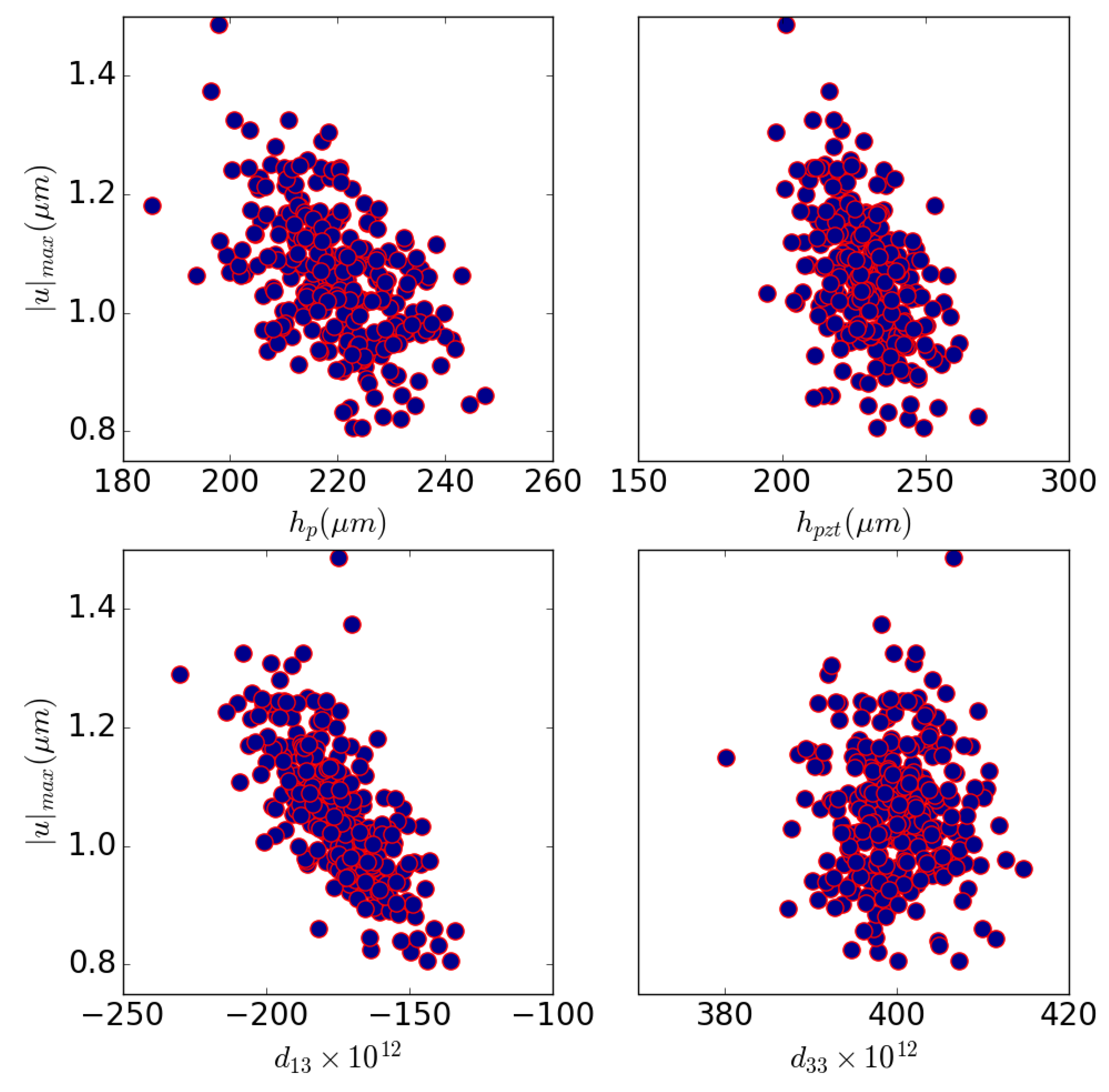
Sensitivity analysis was conducted for maximum center deflection with uncertain variables, as shown in Figure 12, using the Latin hypercube sampling approach [21]. It can be seen from the scatter plots that the response maximum amplitude was more correlated with thicknesses and piezoelectric coefficient $d_{31}$, while correlation with other parameter $d_{33}$ was weak. This is evidently shown in the results of the correlation coefficients for all the parameters in Table 7, where the strongest correlation with $d_{31}$ was observed for different approaches and correlation measures.

4.2.2. Quantification of Numerical Errors

The main numerical error in this current computation was discretization error. To evaluate the discretization error in the Uncertainty Quantification (UQ) framework, numerical simulations were performed on two grid levels for each of the samples. The results from the coarse and fine grids can be used to estimate discretization errors using Richardson’s extrapolation, as stated in Equation (21). Here, for each sampled case, this was carried out on two grid levels of $G_2$ and $G_3$ (Table 6). 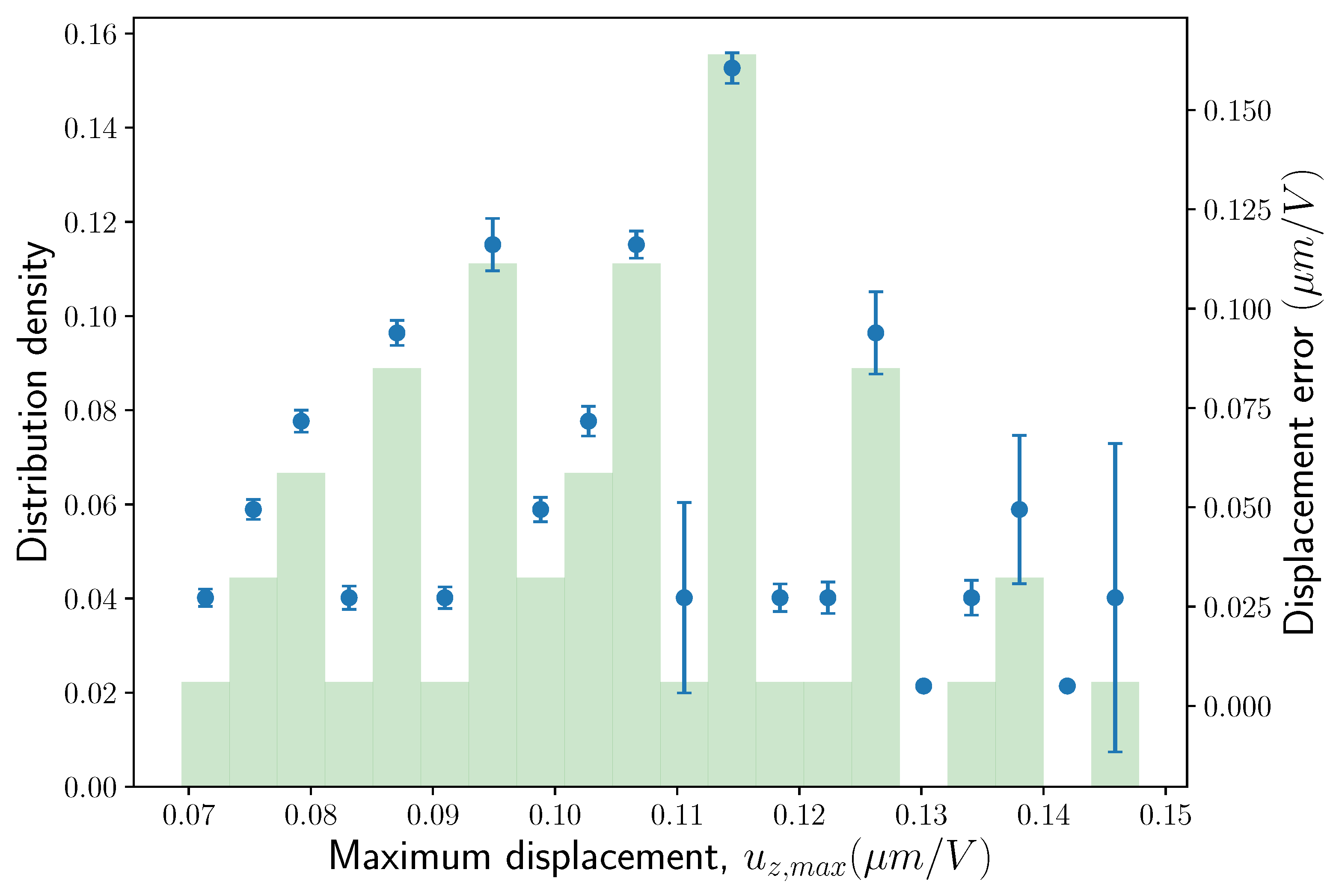Figure 13 shows the distribution of the maximum displacement and estimated numerical error for 200 samples using the Latin hypercube sampling technique. The mean and standard deviation of numerical uncertainty was ${\epsilon }_{h,mean}=3.361$ × 10${}^{-2}$ ($\mathsf{\mu }$m/V) and ${\epsilon }_{h,std}=5.865$ × 10${}^{-3}$ ($\mathsf{\mu }$m/V), respectively.

4.2.3. Propagation of Uncertainties through the Model

Depending on the types of uncertainties, there are different approaches to quantify uncertainty in model predictions [15]. Sampling methods can be used for Uncertainty Quantification (UQ) in which the response characteristic can be obtained from a probability distribution of uncertain inputs. Apart from this sampling-based approach, other UQ methods including polynomial chaos expansion, interval analysis, and reliability were explored to determine the uncertainty of the response.

Table 8. Moments of maximum deflection estimated using different Uncertainty Quantification (UQ) approaches.

Method	No. of Evaluations	Mean ($\mathsf{\mu }$m/V)	Std Dev ($\mathsf{\mu }$m/V)	Skewness	Kurtosis
LHS200	200	1.0755 × 10${}^{-7}$	1.2538× 10${}^{-8}$	1.1756	6.8497
LHS300	300	1.0543 × 10${}^{-7}$	1.1204 × 10${}^{-8}$	2.2445 × 10${}^{-1}$	6.9922 × 10${}^{-1}$
Polynomial chaos expansion	135	1.0543 × 10${}^{-6}$	1.0590 × 10${}^{-7}$	1.5774× 10${}^{-1}$	6.8291 × 10${}^{-2}$

presents the moments of the response (maximum deflection) obtained from using different UQ methods. It can be seen that the mean response predicted by all the methods was consistent, ranging from 0.1031–0.1054 $\mathsf{\mu }$m/V, while the prediction of the standard deviation was more spread using different methods. The global interval analysis approach normally used for quantification of epistemic uncertainties provided a similar response prediction as the LHS-based approach, with much fewer evaluations. 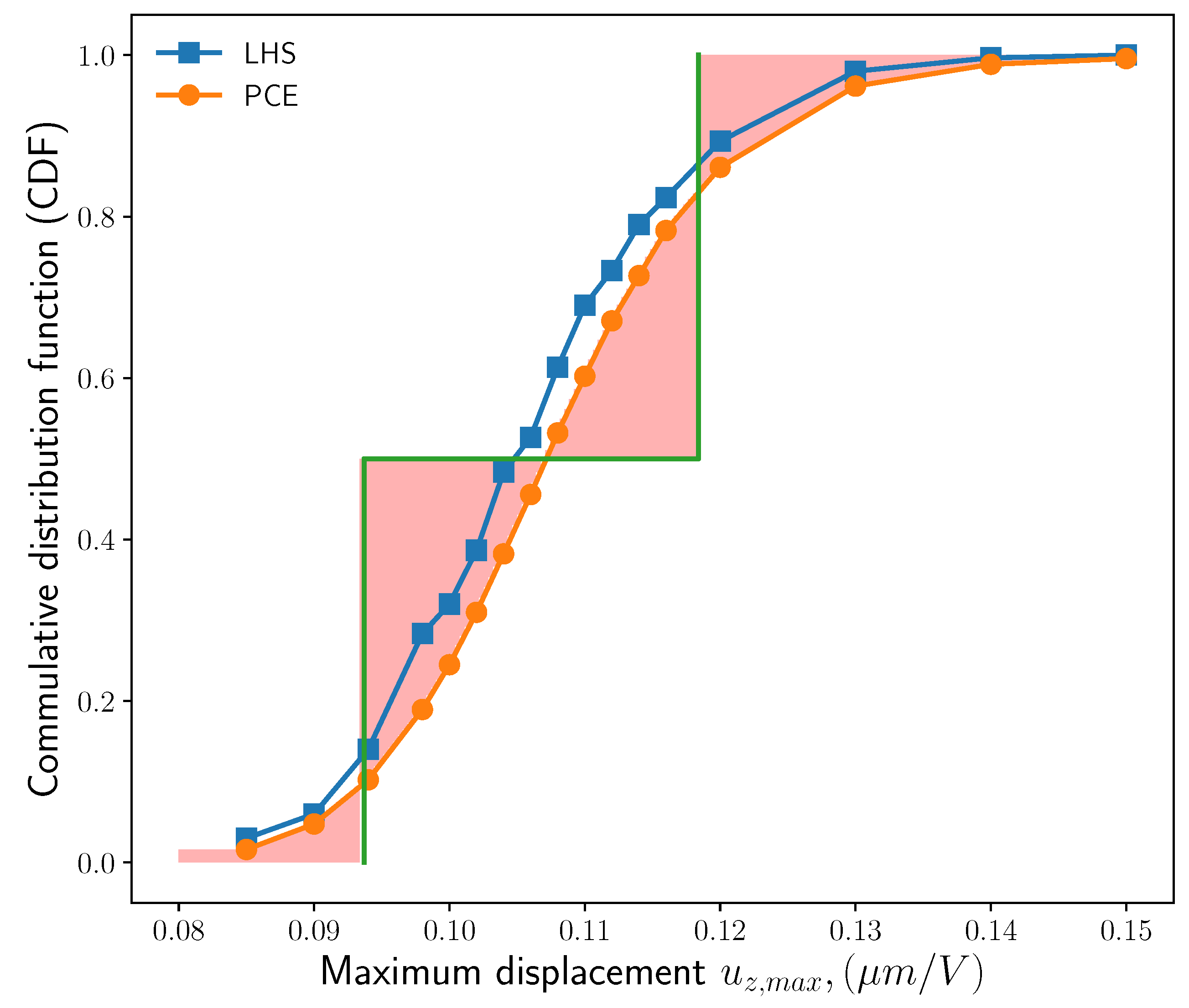Figure 14 depicts the Cumulative Distribution Function (CDF) of maximum deflection where it is less likely ($40\%$) to obtain a response of $u_{max}\le 1.0$, while the probability of obtaining maximum deflection of $u_{max}\le 0.115$ $\mathsf{\mu }$m/V is very likely (80–90%). Results from this UQ confirmed the variations in the responses measured from experiments and provided confidence to the numerical simulations.

4.2.4. Model Uncertainty

The model uncertainty is measured from the error between the model prediction of the quantity of interest and the true value obtained from experiment observation at the same input conditions. With uncertainties in model input, a CDF of the quantity of interest can be obtained when propagating those uncertainties through the model, as shown in Figure 14. Likewise, one can also reconstruct a CDF of experimental observation taking into account the uncertainties with measurement procedures. Here, a crude reconstruction of experimental CDF was performed from two available data points. Following [22], a model validation metric was defined as the intersection area between the two CDF curves:

$${\epsilon }_{model}={\int }_{-\infty }^{\infty }(f_{CDF,e}\left(u_{z,max}\right)-f_{CDF,m}\left(u_{z,max}\right))du.$$

(30)

Among various measures of model errors, the area validation metric provides a good estimation for evidence of disagreement between the model and experiment. It can be computed from a limited number of experimental data; thus making it more suitable for many engineering applications. From the current results of CDF shown in Figure 14, the model error is estimated to be ${\epsilon }_{model}=7.146$ × 10${}^{-3}$ $\mathsf{\mu }$m/V.

From the above estimation of uncertainties, for any given condition, a corrected prediction of maximum displacement can be computed by including both model error and numerical uncertainties:

$$u_{z,max}^c(.)=u_{z,max}^{pred}+{\epsilon }_{num}+{\epsilon }_{model}.$$

(31)

This corrected prediction takes into account various uncertainties in model input, numerical discretization errors, as well as model errors.

5. Conclusions

In this work, we presented the development of a finite element model for simulations of piezoelectric materials. The model was an extension of the traditional nodal-based FEM formulation with an additional unknown for electrical potential. The developed model was verified and validated with experimental data for a number of canonical applications including a single-layer PZT beam to multiple layer plates. It was then used for the characterization of the responses from piezoelectric actuators for synthetic jet devices. It was shown that the responses of the actuators were sensitive to the properties of the piezoelectric layer, resulting in different displacement characteristics of the actuator plates. The FEM model was employed to quantify uncertainties in the response amplitudes of the plate with uncertain input of the material properties of the piezoelectric layer. Results from the uncertainty quantification confirmed fluctuations in the responses measured in the experiment and provided confidence to the developed model. It has been shown that the proposed work can be applied for more complex three-dimensional structures of piezoelectric materials. The model forms a basic building block for a multi-physic simulations of synthetic jet devices by coupling it with a flow solver for fluid-structure interaction analysis. This remains as our future work to apply the model to the design and optimization of the device.

References

1. Piefort, V. Finite Element Modelling of Piezoelectric Active Structures. Ph.D. Thesis, Active Structures Laboratory, Department of Mechanical Engineering and Robotics, Université libre de Bruxelles, Brussels, Belgium, 2001. [Google Scholar]
2. Luna, M.E.S.; Fullam, S. Piezoelectric Heart Rate Sensing for Wearable Devices or Mobile Devices. U.S. Patent 13,672,398, 8 December 2012. [Google Scholar]
3. Rastegar, J.S.; Spinelli, T. Piezoelectric-Based Toe-Heaters for Frostbite Protection. U.S. Patent 12,075,645, 13 March 2008. [Google Scholar]
4. Burns, J.R. Ocean Wave Energy Conversion Using Piezoelectric Material Members. U.S. Patent 4,685,296, 11 August 1987. [Google Scholar]
5. Żyszkowski, Z. Podstawy Elektroakustyki; WNT: Warszawa, Poland, 1984. [Google Scholar]
6. Smits, J.G.; Dalke, S.I.; Cooney, T.K. The Constituent Equations of piezoelectric Bimorph. Sens. Actuators A Phys. 1991, 28, 41–61. [Google Scholar] [CrossRef]
7. Dong, X.J.; Meng, G. Dynamic analysis of structures with piezoelectric actuators based on thermal analogy method. Int. J. Adv. Manuf. Technol. 2006, 27, 841–844. [Google Scholar] [CrossRef]
8. Allik, H.; Hughes, T.J.R. Finite element method for piezoelectric vibration. Int. J. Numer. Methods Eng. 1970, 2, 151–157. [Google Scholar] [CrossRef]
9. Kpeky, F.; Abed-Meraim, F.; Daya, E.M. New linear and quadratic prismatic piezoelectric solid–shell finite elements. Appl. Math. Comput. 2018, 319, 355–368. [Google Scholar] [CrossRef]
10. Carrera, E.; Valvano, S.; Kulikov, G.M. Electro-mechanical analysis of composite and sandwich multilayered structures by shell elements with node-dependent kinematics. Int. J. Smart Nano Mater. 2018, 9, 1–33. [Google Scholar] [CrossRef] [Green Version]
11. Benjeddou, A. Advances in Piezoelectric Finite Element Modeling of Adaptive Structural Elements: A Survey. Comput. Struct. 2000, 76, 347–363. [Google Scholar] [CrossRef]
12. Patzák, B. OOFEM—An object-oriented simulation tool for advanced modeling of materials and structures. Acta Polytech. 2012, 52, 59–66. [Google Scholar]
13. Roache, P.J. Verification of Codes and Calculations. AIAA J. 1998, 36, 696–702. [Google Scholar] [CrossRef]
14. Oberkampf, W.L.; DeLand, S.M.; Rutherford, B.M.; Diegert, K.V.; Alvin, K.F. Error and uncertainty in modeling and simulation. Reliab. Eng. Syst. Saf. 2002, 75, 333–357. [Google Scholar] [CrossRef]
15. Helton, J.C.; Johnson, J.D.; Oberkampf, W.L. An exploration of alternative approaches to the representation of uncertainty in model predictions. Reliab. Eng. Syst. Saf. 2004, 85, 39–71. [Google Scholar] [CrossRef]
16. Mahadevan, S.; Liang, B. Error and Uncertainty Quantification and Sensitivity Analysis in Mechanics Computational Models. Int. J. Uncertain. Quantif. 2011, 1, 147–161. [Google Scholar] [CrossRef]
17. Mieczkowski, G. The constituent equations of piezoelectric cantilevered three-layer actuators with various external loads and geometry. J. Theor. Appl. Mech. 2017, 55, 69–86. [Google Scholar] [CrossRef]
18. Prasad, S.; Sankar, B.; Cattafesta, L.; Horowitz, S.; Gallas, Q.; Sheplak, M. Two-Port Electroacoustic Model of a Piezoelectric Circular Composite Plate. In Proceedings of the 43rd AIAA/ASME/ASCE/AHS/ASC Structures, Structural Dynamics, and Materials Conference, Denver, CO, USA, 22–25 April 2002; American Institute of Aeronautics and Astronautics: Reston, VA, USA, 2002. [Google Scholar]
19. Prasad, S.A.; Gallas, Q.; Horowitz, S.B.; Homeijer, B.D.; Sankar, B.V.; Cattafesta, L.N.; Sheplak, M. Analytical Electroacoustic Model of a Piezoelectric Composite Circular Plate. AIAA J. 2006, 44, 2311–2318. [Google Scholar] [CrossRef]
20. APC International. Physical and Piezoelectric Properties of APC Materials; APC International: Mackeyville, PA, USA, 2013; pp. 841–842. [Google Scholar]
21. Adams, B.M.; Ebeida, M.S.; Eldred, M.S.; Jakeman, J.D.; Swiler, L.P.; Eddy, J.P. Dakota, A Multilevel Parallel Object-Oriented Framework for Design Optimization, Parameter Estimation, Uncertainty Quantification, and Sensitivity Analysis Version 6.7 Theory Manual. Sandia Technical Report SAND2014-4633; 2014. Available online: https://dakota.sandia.gov/sites/default/files/docs/6.7/Theory-6.7.0.pdf (accessed on 20 November 2018).
22. Roy, C.J.; Oberkampf, W.L. A comprehensive framework for verification, validation, and uncertainty quantification in scientific computing. Comput. Methods Appl. Mech. Eng. 2011, 200, 2131–2144. [Google Scholar] [CrossRef]
Figure 1. Schematic of hexahedral (LSPiezo) and tetrahedral (LTRPiezo) reference element for piezo-elastic coupling implemented in OOFEM.
Computation 06 00060 g001
Figure 2. Single-layer beam. The poling direction of the beam is the z-axis. The length L, height H, and width D of the beam are 10 mm, 2 mm, and 5 mm, respectively.
Computation 06 00060 g002
Figure 3. Single-layer beam under tensile and shear displacement.
Computation 06 00060 g003
Figure 4. Bimorph beam with equally-thick piezoelectric layers.
Computation 06 00060 g004
Figure 5. Comparison of FEM results with analytical data for the bimorph beam case: (a) deflection profile along the x-axis and (b) deflection error along the length of the bimorph beam with the increasing number of elements in the simulation.
Computation 06 00060 g005
Figure 6. Three-layered beam with two smaller piezoelectric beams of the same width (shown as gray color) as the non-piezoelectric beam (shown as white color). Beam length L = 60 mm; piezoelectric layer thickness t p = 0.5 mm, and the thickness of the non-piezoelectric beam was t b = 1.0 mm; and the applied voltage v = 100 V.
Computation 06 00060 g006
Figure 7. Comparison of FEMwith analytical results for the three-layer beam case: (a) deflection profile along the beam span and (b) error of deflection for meshes with different numbers elements.
Computation 06 00060 g007
Figure 8. Problem setup and computational domain of the composite piezoelectric actuator. Note that the computational domain is taken as a quarter of the disc with symmetric planes.
Computation 06 00060 g008
Figure 9. Mesh convergence of FEM analysis for a unimorph piezoelectric actuator in comparison with the experiment and analytical results [18]. The plots show the deflection profile with normalized radius along the bottom shim plate.
Computation 06 00060 g009
Figure 10. Comparison of different experimental data and FEM results obtained from the present work on the same device APC 850 reported in [18,19]. Here, the experimental (circle symbols) and numerical data (dashed line with square symbols) are shown for two different setups of the same device.
Computation 06 00060 g010
Figure 11. Prediction of maximum deflection at the center of the plate as a function of the radius ratio between the PZT layer and shim layer. The comparison between analytical and current FEM model for different thickness ratios h p / h s shows a consistent trend in the variation of maximum displacement with the radius ratio.
Computation 06 00060 g011
Figure 12. Scatter plot of maximum deflection at the center of the disc with geometrical and material property parameters using the Latin hypercube sampling technique.
Computation 06 00060 g012
Figure 13. Distribution of the maximum response with uncertainties and its numerical discretization error obtained from Richardson extrapolation. The displacement error is shown as error bars in the graph.
Computation 06 00060 g013
Figure 14. Cumulative distribution function of the maximum deflection response obtained from different UQ approaches. The green line is the CDF of the experiment constructed from two data points. The shaded area is the area validation metric.
Computation 06 00060 g014