Review

Recent Progress in First-Principles Methods for Computing the Electronic Structure of Correlated Materials

Department of Physics, Division of Mathematical Physics, Lund University, Professorsgatan 1, 223 63 Lund, Sweden
*
Author to whom correspondence should be addressed.
Computation 2018, 6(1), 26; https://doi.org/10.3390/computation6010026
Submission received: 27 February 2018 / Revised: 12 March 2018 / Accepted: 13 March 2018 / Published: 19 March 2018
(This article belongs to the Special Issue In Memory of Walter Kohn—Advances in Density Functional Theory)

Abstract

:
Substantial progress has been achieved in the last couple of decades in computing the electronic structure of correlated materials from first principles. This progress has been driven by parallel development in theory and numerical algorithms. Theoretical development in combining ab initio approaches and many-body methods is particularly promising. A crucial role is also played by a systematic method for deriving a low-energy model, which bridges the gap between real and model systems. In this article, an overview is given tracing the development from the LDA+U to the latest progress in combining the G W method and (extended) dynamical mean-field theory ( G W +EDMFT). The emphasis is on conceptual and theoretical aspects rather than technical ones.

1. Introduction

One of the keys in understanding physical properties of a material is its electronic structure. The electronic structure determines essentially all physical properties including structural, optical, magnetic, as well as transport properties. Since the advent of density functional theory (DFT) [1,2] some fifty years ago, tremendous progress has been attained in obtaining details in the electronic structure of complex materials crucial for not only understanding many physical phenomena, but also for predicting new physical properties. The success of DFT relies greatly on the local density approximation (LDA) [2] and its subsequent development through the generalized gradient approximation (GGA) [3], and, more recently, the hybrid functional [4], involving a non-local exchange potential that takes DFT a step towards the self-energy in Green’s function theory [5].
The physical and chemical properties of a material are dictated to a large extent by the valence electrons that form states around the Fermi surface. Inspection of the periodic table reveals two kinds of valence electrons, itinerant and semi-itinerant or localized electrons, the former form broad bands whereas the latter narrow bands. The first type may be identified with electrons originating from the s atomic orbitals found in simple metals such as aluminium and sodium or from p orbitals found in semiconductors such as silicon and gallium arsenide. The second type may be associated with electrons originating from 3 d orbitals (transition metals) or 4 f orbitals (lanthanides). For materials with valence electrons of s or p character, the one-particle LDA works very well, although some shortcomings such as too small band gaps are well known [6]. For materials in which the valence states are dominated by the 3 d or 4 f electrons, the LDA is more prone to failure. This failure can to a certain extent be traced back to the strong orbital polarization associated with electron localization as found in 3 d and 4 f elements [7]. Whereas the electronic structure of pure transition metals (e.g., iron and nickel), in which the 3 d electrons are relatively itinerant, can be described quite well within the LDA, the electronic structure of insulating transition metal oxide compounds, in which the 3 d electrons undergo localization due to the strong onsite Coulomb repulsion, are often wrongly predicted to be metallic within the LDA. A well-known example is NiO, which is regarded as a prototype of the so-called Mott–Hubbard insulators [8].
In the last few decades, a wide variety of new materials hosting numerous intriguing properties have been experimentally discovered and synthesized. Perhaps the most familiar of these is the high-temperature superconducters [9] discovered in the mid-nineteen eighties by Berdnoz and Müller [10]. Another example is provided by materials with colossal magnetoresistance [11] in which the large change in magnetoresistivity upon application of a magnetic field has been utilized in industrial applications as hardisks in our computers. A common characteristic of these materials is the possession of large susceptibility: a small change in the external perturbation causes a large change in the corresponding physical quantity to which the perturbation is coupled. This property is related to the fact that many of these materials are close to phase transitions such as the metal-to-insulator transition. These materials belong to a class of materials known as strongly correlated, which may be loosely defined as those systems for which conventional theories based on the one-electron or mean-field picture such as the LDA fail or is insufficient in describing their electronic structure. The valence states of these materials are characterized by a set of partially filled narrow bands usually originating from 3 d orbitals of transition metals or 4 f orbitals of lanthanides embedded in relatively broad bands. An important consequence of these narrow bands is that the Coulomb repulsion among the electrons occupying these bands becomes comparable to or larger than the kinetic energy. In other words, the ratio between the Coulomb repulsion and the bandwidth becomes significantly larger than one. For this reason, a proper treatment of the Coulomb interaction is necessary and mean-field or one-particle theories such as the LDA are no longer sufficient to describe the electronic structure. This poses a difficult theoretical problem and the usual approach is to resort to the Hubbard model and the Anderson impurity model. These models, however, assume some input parameters in the form of tight-binding hopping parameters and the Hubbard U representing the effective Coulomb repulsion of the localized electrons. While the model approach is useful for gaining qualitative understanding and insights into the physics of electron correlations, it lacks quantitative predictive capability. Moreover, great care must be taken when constructing a model in order to avoid misleading results when the model does not faithfully represent the system under investigation. A fully first-principles description of the electronic structure of correlated materials is undoubtedly one of the great challenges in modern condensed matter physics.
The purpose of this article is to present a short overview of the recent development in first-principles methods for computing the electronic structure of correlated materials for which commonly used mean-field methods either fail or are insufficient. Particular emphasis is put on those methods that combine traditional band structure methods with many-body approaches since this path has proven to be fruitful. This line of approach has a long history, starting in the late eighties with the idea of incorporating the Hubbard interaction in the background LDA Hamiltonian resulting in the widely used LDA+U method [7,12,13]. The arrival of dynamical mean-field theory (DMFT) [14,15,16] in the late nineties provides a new impetus to go beyond LDA+U by including dynamical effects of the onsite self-energy beyond the static Hartree–Fock approximation, resulting in the highly successful LDA+DMFT method [17,18,19,20]. Parallel to this development, the G W approximation (GWA) [6,21,22,23], which is a more traditional many-body perturbation theory (diagrammatic approach) based on Hedin’s expansion of the self-energy in the renormalized screened interaction, offers a better starting band structure than the LDA. While DMFT provides an improvement on the U side, the GWA furnishes a better background band structure by including long-range correlations on top of which strong onsite electron correlations can be further incorporated. This naturally leads to the G W +DMFT scheme [24], a combination of the GWA and DMFT. Several simplified approaches based on or related to the G W +DMFT scheme have since been proposed [25,26,27,28,29] and self-consistent calculations for model systems have been carried out [30,31,32,33,34,35,36,37], but, only recently, self-consistent G W +DMFT has been performed for real materials [38,39]. In the next section, a survey of the development leading to the present state-of-the-art schemes is described followed by a relatively detailed description of the G W +DMFT scheme, which is a basis for simplifications and further development. Simplified G W +DMFT schemes and related schemes are also discussed as well as applications of these new schemes to some materials, which are relatively few since all these schemes are rather new. The article is concluded with future prospects and directions. We do not discuss technical aspects such as basis functions and computational methods but rather focus on the conceptual and theoretical aspects. We do not attempt to be comprehensive but rather focus on a particular line of development. References are made to those works that are directly related to the topics discussed in the article so they are not meant to be comprehensive either.

2. Theoretical Background and Historical Development
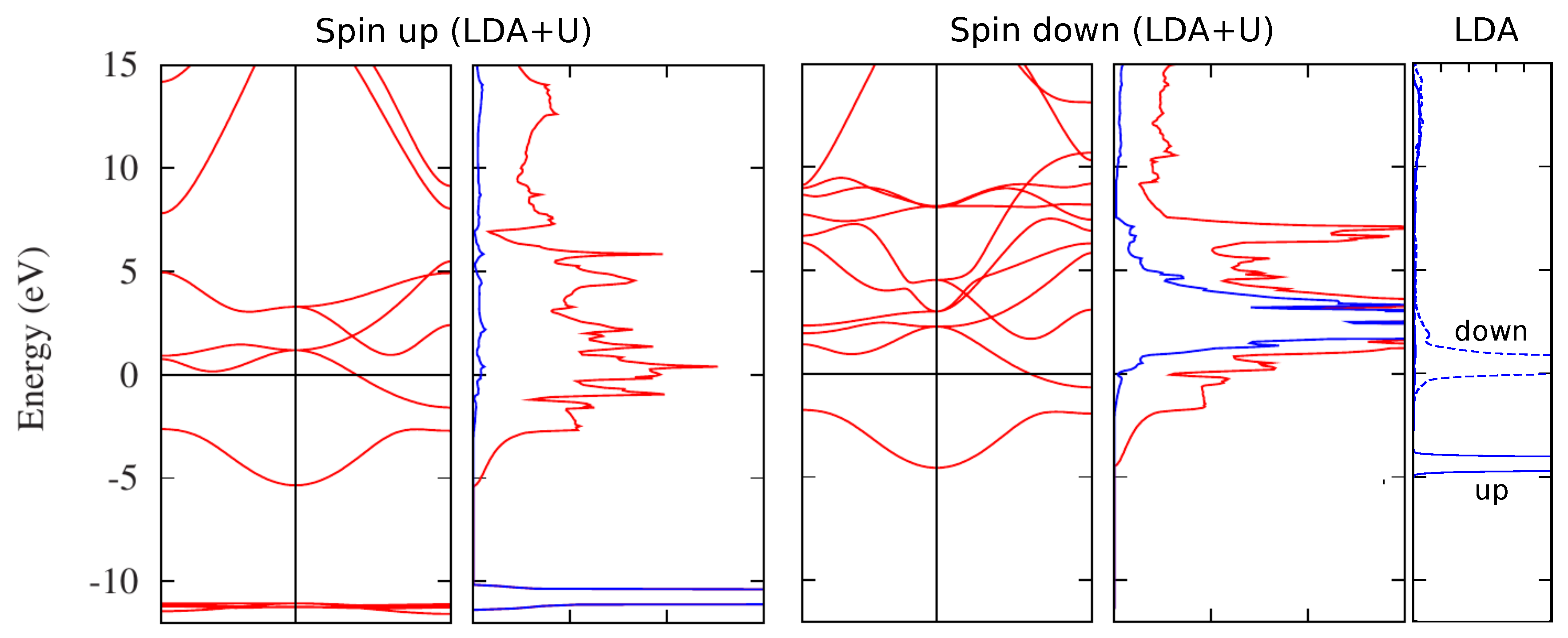
Modern electronic structure theory starting from the arrival of DFT onward is preceded by early theories, prominently the Hartree and Hartree–Fock approximations. Slater in the early fifties introduced the idea of localizing the non-local exchange potential with the X α method [40,41], which may be regarded as a precursor to DFT. The reduction of a non-local to a local potential evidently brings a lot of numerical simplifications. However, one drawback with a local potential is that every electron experiences the same potential irrespective of which state the electron occupies:
1 2 2 + V ( r ) ψ k ( r ) = ε k ψ k ( r ) .
In the Kohn–Sham equation of DFT, the mean-field V is the Kohn–Sham potential V K S , which is the sum of the external field from the nuclei V e x t , the Hartree potential of the electrons V H , and the so-called exchange-correlation potential V x c :
V K S = V e x t + V H + V x c .
Although the Kohn–Sham eigenvalues ε k do not have a clear physical meaning except for the highest occupied, it is nevertheless common practice to interpret them as one-particle excitation energies observed in an angle-resolved photoemission experiment. The Kohn–Sham potential V K S is a local potential, which is expected to work well for electrons occupying extended states, such as those originating from s and p orbitals, since they mainly experience the average field of all the other electrons. Indeed, the bands arising from these extended states usually resemble free-electron bands with some modifications due to the crystal structure as well as renormalization of the bandwidth. A valence electron originating from 3d or 4f orbital on the other hand is rather localized in space around an atom to which the associated orbital belongs. The Coulomb repulsion among these electrons is large and often leads to orbital polarization meaning that the occupation numbers of the angular momentum components differ significantly from the average value. For example, a transition metal atom in a transition metal oxide is at the center of an octahedral cage with oxygen atoms at its corners. The breaking of the rotational symmetry in the cubic environment lifts the degeneracy of the 3 d orbitals into the e g and t 2 g symmetry with the e g states usually lying higher than the t 2 g states. Although this orbital polarization can be achieved by a local potential, it is less effective than a non-local potential. In practice, a local potential as in the LDA may not be sufficiently flexible to induce a strong orbital polarization. When the orbital polarization is not strong enough to energetically separate the orbitals with different angular momentum component (m quantum number), all orbital components may be partially occupied, yielding a metallic state instead of the experimentally observed insulating state.
In addition to the average mean-field of the other electrons, there is a non-local and state-dependent interaction with other electrons. This additional non-local interaction is the self-energy, which depends explicitly on the positions of the other electrons as well as on their dynamics:
1 2 2 + V e x t ( r ) + V H ( r ) ψ k ( r ) + d r 3 Σ ( r , r ; E k ) ψ k ( r ) = E k ψ k ( r ) .
The non-local and energy-dependent self-energy Σ is a central quantity in electronic structure theory. The LDA exchange-correlation potential in density functional theory may be regarded as a local and static approximation to this self-energy. To improve the LDA is then equivalent to finding a better approximation for the self-energy.

2.1. LDA+U

To handle cases containing 3 d or 4 f partially filled bands in which there is a large non-local interaction between the localized electrons, it is usual to employ the Hubbard model, which, in its simplest form with one orbital per site, takes the form:
H = i j , σ t i j c i σ c j σ + U i n i n i .
The first term describes electron hopping from site i to j, which corresponds to the one-particle band structure, whereas the second term takes into account explicitly the Coulomb interaction between electrons with the opposite spin occupying the same orbital, which cannot be reduced to a one-particle term. Following the Hubbard model, it would seem physically motivated to introduce a Hubbard U term on top of the LDA total energy [7,12,13]:
E = E L D A + U 2 i j n i n j U N ( N 1 ) / 2 , ,
where n i ’s are the occupation numbers of the localized orbitals in an open 3 d / 4 f shell and N is the total number of 3 d / 4 f electrons: N = i n i . Here, the subscript i may include the spin index. In principle, we may replace E L D A with a more accurate total energy approximation such as E G G A . Assuming that the LDA or GGA total energy is accurate, the last term, which is the electrostatic Coulomb energy, is subtracted to cancel the average energy of the second term. This last term is referred to as the double-counting term.
The orbital energy is given by
ε i = E n i = ε i L D A + U ( 1 2 n i ) .
For an occupied orbital, n i = 1 , so that the LDA orbital energy is pushed down by U / 2 , whereas, for an unoccupied orbital, n i = 0 so that the orbital is pushed up by U / 2 , resulting in the formation of the lower and upper Hubbard bands. The LDA+U potential experienced by orbital i is given by
V i L D A + U = V i L D A + U ( 1 2 n i ) .
For a multi-orbital system, the LDA+U functional is given by
E L D A + U [ ρ σ ( r ) , { n σ } ] = E L D A [ ρ σ ( r ) ] + E U [ { n σ } ] E d c [ { n σ } ] ,
where E L D A is the spin-density functional energy. n σ is the density matrix defined by
n m m σ = 1 π E F d ω Im G i n l m , i n l m σ ( ω ) ,
where
G i n l m , i n l m σ ( ω ) = i n l m σ | ( ω H ^ ) | i n l m σ
is the Green function in the local orbital representation i n l m σ with i denoting the atomic site, n the main quantum number, l the orbital angular momentum, m the z-component of the angular momentum, and σ the spin. The last two terms in the LDA+U functional are defined only within the subspace of the localized orbitals:
E U [ { n σ } ] = 1 2 { m } , σ m , m | V e e | m , m n m m σ n m m σ + ( m , m | V e e | m , m m , m | V e e | m , m ) n m m σ n m m σ ,
E d c [ { n σ } ] = 1 2 U N ( N 1 ) 1 2 J σ N σ ( N σ 1 ) .
V e e is the screened Coulomb interaction among the electrons residing in the subspace formed by the localized orbitals, N σ = Tr ( n σ ) , N = σ N σ and U and J are the screened Coulomb and exchange parameters. The Coulomb matrix elements are defined according to
m 1 , m 2 | V e e | m 3 , m 4 = d 3 r d 3 r φ m 1 * ( r ) φ m 3 ( r ) V e e ( r , r ) φ m 4 ( r ) φ m 2 * ( r ) .
The Hamiltonian defining the Green function is the LDA Hamiltonian supplemented by a term arising from E U E d c :
H σ = H L D A σ + m m i n l m σ V m m σ i n l m σ ,
where
V m m σ = δ δ n m m σ ( E U E d c ) = { m } m , m | V e e | m , m n m m σ r + ( m , m | V e e | m , m m , m | V e e | m , m ) n m m σ U ( N 1 2 ) + J ( N σ 1 2 ) .
The additional potential on top of the LDA potential arising from the Hubbard U term clearly displays its non-local and state-dependent property similar to the exchange potential. The matrix elements m , m | V e e | m , m can be related to U and J via the Slater integrals. Often, U and J are treated as adjustable parameters, but it is possible to estimate them using the constrained LDA method [42,43]. Alternatively, it is possible to compute the matrix elements m , m | V e e | m , m directly using the constrained random-phase approximation (cRPA) method described in the Appendix A. U and J can then be extracted naturally from these matrix elements as the onsite Coulomb interaction and exchange integrals.
The LDA+U scheme has been very successful in improving the LDA electronic structure of strongly correlated systems, and it is now widely used due to its success and simplicity. An illustration of the effect of the Hubbard U term on the LDA band structure is given in the case of gadolinium (Figure 1) in which the majority spin channel of the 4f states is fully occupied, whereas the minority channel is completely empty. In the LDA, the separation between these two spin states is severely underestimated, which illustrates the importance of a non-local potential. The Hubbard U term is expected to pull down the occupied 4 f band and push up the unoccupied one. As can be seen in the figure, the LDA+U scheme substantially increases the separation between the occupied and unoccupied 4 f bands yielding a much better agreement with experiment [7,44].
The seminal idea of introducing the Hubbard U term into the LDA Hamiltonian has exerted a far reaching influence on later development of the electronic structure of strongly correlated systems. The LDA+U scheme, however, is not without shortcomings. The most serious approximation is the assumption that the self-energy beyond the exchange-correlation LDA potential is static. For this reason, it is not possible to describe the spectral function of a correlated metal that consists of a quasiparticle peak around the Fermi level sandwiched by incoherent satellite features. These satellites are a consequence of the dynamics or energy-dependence of the self-energy and cannot be reproduced by a static theory. To include dynamical effects of the self-energy, it is natural to combine LDA and DMFT, to be described in a later section, but we first outline the G W and DMFT methods in the next two sections.

2.2. The G W Method

The LDA+U method is in some way phenomenological since it is not derived from a basic theoretical premise. A theoretically rigorous approach for computing the self-energy is to use Green’s function approach, which is designed to yield the one-particle excitation energies corresponding to the band structure observed in an angle-resolved photoemission experiment. Within the traditional many-body perturbation technique, the self-energy is expanded in powers of the Coulomb interaction v ( r r ) . It was shown by Hedin [21] that it is possible to re-sum the perturbation expansion so that the perturbation expansion of the self-energy is expressed in powers of the screened interaction W, which is an energy-dependent quantity. The first order term in this expansion is the well-known GWA [6,21,23], which consists of the bare exchange and a correlation part that takes into account the dynamic response of the electrons in the form of screening. Screening effects are especially important in large molecules and crystalline solids and account for the reduction of the band gap in semiconductors and insulators and remove the unphysical zero density of states at the Fermi level in metals within the Hartree–Fock approximation.
In the Green’s function approach [47], the Fock exchange is expressed as
Σ x ( r , r ) = i G ( r t , r t ) v ( r r ) δ ( t t ) ,
where the non-interacting Green’s function is given by
G ( r , r ; t t ) = i θ ( t t ) k o c c ψ k ( r ) ψ k * ( r ) e i ε k ( t t ) i θ ( t t ) k u n o c c ψ k ( r ) ψ k * ( r ) e i ε k ( t t ) .
Its Fourier transform in frequency space, G ( r , r ; ω ) = d t exp ( i ω t ) G ( r , r ; t ) is given by
G ( r , r ; ω ) = k o c c ψ k ( r ) ψ k * ( r ) ω ε k i δ + k u n o c c ψ k ( r ) ψ k * ( r ) ω ε k + i δ .
The wave functions and eigenvalues ψ k , ε k are usually taken to be those of the LDA. Using this expression in Equation (16) and using the rule that equal-time Green’s function implies G ( r t , r t ) = G ( r t , r t + ) , where t + is infinitessimally later than t, we obtain the familiar form of the exchange potential:
Σ x ( r , r ) = v ( r r ) k o c c ψ k ( r ) ψ k * ( r ) .
Heuristically, the GWA [6,21,23,48] may be obtained by replacing the bare Coulomb interaction v with a screened Coulomb interaction W:
Σ G W ( r , r ; t t ) = i G ( r , r ; t t ) W ( r , r , t t ) .
After Fourier transformation, we find
Σ G W ( r , r ; ω ) = i d ω 2 π G ( r , r ; ω + ω ) W ( r , r ; ω ) e i ω η .
To calculate W ( r , r , t t ) or W ( r , r ; ω ) , we first consider applying an arbitrary external perturbation V e x t ( r , t ) . According to linear response theory, the induced density is given by
ρ i n d ( r , t ) = d 3 r d t R ( r t , r t ) V e x t ( r , t ) .
This induced density in turn generates a back potential
V i n d ( r , t ) = d 3 r v ( r r ) ρ i n d ( r , t ) ,
which screens the applied perturbation V e x t resulting in a screened potential V s c r :
V s c r ( r , t ) = V e x t ( r , t ) + V i n d ( r , t ) = V e x t ( r , t ) + d 3 r 1 v ( r r 1 ) ρ i n d ( r 1 , t ) = V e x t ( r , t ) + d 3 r 1 v ( r r 1 ) d 3 r 2 d t 2 R ( r 1 t , r 2 t 2 ) V e x t ( r 2 , t 2 ) .
Schematically, we may write
V s c r = ( 1 + v R ) V e x t
and recognize that 1 + v R is the inverse dielectric matrix ϵ 1 .
If we now regard v ( r r ) δ ( t t ) = δ ( t t ) / | r r | , which is an instantaneous Coulomb potential arising from a point charge at r , as our external perturbation with ( r , t ) treated as a parameter, we then arrive at
W ( r , r ; t t ) = v ( r r ) δ ( t t ) + d 3 r 1 v ( r r 1 ) d 3 r 2 d t 2 R ( r 1 t , r 2 t 2 ) v ( r 2 r ) δ ( t 2 t ) = v ( r r ) δ ( t t ) + d 3 r 1 d 3 r 2 v ( r r 1 ) R ( r 1 , r 2 , t t ) v ( r 2 r ) .
We have made use of the fact that the response function R depends only on relative time for a system with time-independent Hamiltonian. We note that v ( r r 1 ) appearing in the integral in the above equation plays a different role than v ( r r ) δ ( t t ) , which plays the role of the external perturbation. This equation reveals the physical meaning of W ( r , r ; t t ) as a time-dependent screened interaction of a Coulomb potential arising from an instanteneous point charge at ( r , t ) . Since
δ ( t t ) = d ω 2 π exp [ i ω ( t t ) ] ,
for each Fourier component of the external perturbation, v ( r r ) exp [ i ω ( t t ) ] , the corresponding Fourier component of the screened interaction is then calculated from the following equation:
W ( r , r ; ω ) = v ( r r ) + d 3 r 1 d 3 r 2 v ( r r 1 ) R ( r 1 , r 2 ; ω ) v ( r 2 r ) .
While the above equation is exact, in practice, we need to resort to approximation in order to compute the response function. A commonly used approximation is the random-phase approximation (RPA) [49] based on the assumption that the system reponds to the total perturbation (external plus back potential) as if the system were non-interacting. If P is the non-interacting response function, then, within the RPA, the induced charge is given by
ρ i n d = R V e x t = P ( V e x t + V i n d ) .
Since V i n d = v ρ i n d = v R V e x t , we then find
R V e x t = P ( V e x t + v R V e x t ) = P ( 1 + v R ) V e x t .
Since the response function is a property of the system independent of the external perturbation, we obtain
R = P + P v R ,
and writing out the variables,
R ( r , r ; ω ) = P ( r , r ; ω ) + d r 1 3 d r 2 3 P ( r , r 1 ; ω ) v ( r 1 r 2 ) R ( r 2 , r ; ω ) .
This equation is actually valid also for the exact response function, but, within the RPA, the polarization function P is approximated by the following expression:
P ( r , r ; ω ) = i d ω 2 π G ( r , r ; ω + ω ) G ( r , r ; ω ) .
When a non-interacting Green’s function as in Equation (18) is used, one obtains the well-known expression:
P ( r , r ; ω ) = k occ k unocc ψ k * ( r ) ψ k ( r ) ψ k * ( r ) ψ k ( r ) ω ε k + ε k + i δ ψ k ( r ) ψ k * ( r ) ψ k ( r ) ψ k * ( r ) ω + ε k ε k i δ .
By using Equation (32) in Equation (28), the screened interaction can be shown to fulfill a similar equation as that of R:
W ( r , r ; ω ) = v ( r r ) + d r 1 3 d r 2 3 P ( r , r 1 ; ω ) v ( r 1 r 2 ) W ( r 2 , r ; ω ) .
The physical meaning of the G W approximation can be understood by evaluating the real part of the self-energy, which can be split into the screened-exchange term Σ S E X and the Coulomb-hole term Σ C O H [21]:
Re Σ S E X ( r , r ; ω ) = k o c c ψ k ( r ) ψ k * ( r ) Re W ( r , r ; ω ε k ) ,
Re Σ C O H ( r , r ; ω ) = k ψ k ( r ) ψ k * ( r ) P 0 d ω π Im W ( r , r ; ω ) ω ε k ω .
The first term has exactly the same form as the familiar Fock exchange in Equation (19) except that the bare Coulomb interaction has been replaced by an energy-dependent screened interaction. The second term involves a sum over all states and can be understood by making an approximation ω ε k 0 , which reduces the expression into
Σ C O H ( r , r ) 1 2 δ ( r r ) W ( r , r ; 0 ) v ( r r ) ,
representing an interaction energy between a quasiparticle (the delta function) and the induced potential from the surrounding screening charge ( W v ).
The success of the G W method is illustrated in Figure 2, which shows that the well-known band gap underestimation of the LDA is almost entirely cured by the G W approximation. Numerous quasiparticle band structure calculations for weakly to moderately correlated materials have also shown good agreement with experimental data. However, for strongly correlated systems, the G W approximation has been found to be insufficient.
G W calculations are usually performed using a non-interacting Green’s function with eigenfunctions and eigenenergies obtained from the LDA. Evidently, the result may differ depending on the starting Green’s function. Early fully self-consistent calculations for the electron gas yielded discouraging results in which the quasiparticle bandwidth widens compared to the free-electron dispersion [59]. Moreover, the plasmon satellites almost vanish. Both of these results are contrary to what one would expect and in disagreement with the experimental results on the alkalis for which the electron gas can be regarded as a good model. The ambiguity in the starting Green’s function motivates the search for a self-consistent scheme that retains the good results obtained when using the LDA Green’s function. This leads to the quasiparticle self-consistent scheme, in which the Green’s function takes the form of a non-interacting Green’s function but constructed from quasiparticle wave functions and energies [60]. This approach generally improves the one-shot G W results, but it has a tendency to overestimate band gaps. Qualitatively, this may be understood by the increase in the band gap after the first iteration, which reduces screening that in turn increases the band gap further in the next iteration yielding a too large band gap after self-consistency is achieved. From computational point of view, the self-consistency cycle is costly and, for this reason, this approach is not widely used in practice.
Another serious problem with the GWA is its failure in describing properly systems in which onsite correlations are strong. A clear example is provided by the much studied cerium α γ isostructural phase transition in which the drastic reduction of the quasiparticle weight from the α -phase to the larger volume γ -phase is not captured (Figure 3) [61]. In general, the Mott metal-insulator transition is also not correctly described, which is a consequence of the neglect of strong onsite correlations in the GWA.

2.3. Dynamical Mean-Field Theory

The G W method is based on a many-body perturbation expansion that has limitations when the electrons are localized so that the onsite Coulomb interaction becomes strong in comparison to the electron kinetic energy as measured by the bandwidth. For this situation, it is physically more sensible to start from the atomic rather than the band structure picture. A commonly used model to describe the electronic structure of localized or semi itinerant electrons is the lattice Hubbard model:
H = i j , σ t i j c i σ c j σ + U i n i n i .
In DMFT [14,15,16], the lattice problem is reduced to an effective impurity problem involving an atomic site in which the onsite Coulomb interaction U is retained, whereas the effects of the Coulomb interaction on other sites are approximated as an effective mean field. Since Coulomb interaction is taken into account only on the impurity site, the resulting self-energy is local (onsite). The effective onsite model is then akin to the Anderson impurity model (AIM) [62]:
H A I M = k σ ε ˜ k a k σ a k σ + k σ ( V k a k σ c 0 σ + V k * c 0 σ a k σ ) μ σ c 0 σ c 0 σ + U n 0 n 0 .
The operators c 0 σ , c 0 σ represent the impurity electrons whereas a k σ , a k σ represent the electrons in the surrounding lattice or the bath. The subscript k corresponds to momentum rather than site index. The first term describes the band structure of the bath electrons surrounding the impurity. The matrix element V k describes the hopping between the impurity site and the bath electrons, simulating the effects of the Coulomb interactions on sites other than the impurity. The retarded Green’s function is a solution to the following operator equation:
( i ω n H ^ A I M ) G ^ ( i ω n ) = 1 .
For the non-interacting Anderson impurity model, i.e., without the last term U n 0 n 0 , taking appropriate matrix elements yields the coupled equations
( i ω n + μ ) G 0 ( i ω n ) = 1 + k V k * G k 0 ( i ω n ) ,
( i ω n ε ˜ k ) G k 0 ( i ω n ) = V k G 0 ( i ω n ) ,
where G 0 = G 00 . Eliminating G k 0 leads to the following result
G 0 1 ( i ω n ) = i ω n + μ d ω Δ ( ω ) i ω n ω ,
Δ ( ω ) = k σ | V k | 2 δ ( ω ε ˜ k ) .
G 0 is the effective mean field of the impurity problem, which is not to be confused with a non-interacting Green’s function. The effective action is then given by
S e f f = 0 β d τ 0 β d τ σ c 0 σ ( τ ) G 0 1 ( τ τ ) c 0 σ ( τ ) + U 0 β d τ n 0 ( τ ) n 0 ( τ ) .
To compute the lattice Green’s function, an assumption is made that the lattice self-energy is equal to the impurity self-energy on every site, i.e., the self-energy is assumed to be local or onsite:
G ( k , i ω n ) = 1 i ω n + μ ϵ k Σ i m p ( i ω n ) .
By solving the impurity Green’s function G i m p of the effective impurity problem defined by S e f f the local impurity self-energy Σ i m p ( i ω n ) is calculated according to
Σ i m p ( i ω n ) = G 0 1 ( i ω n ) G i m p 1 ( i ω n ) .
A crucial ingredient in DMFT is the self-consistency condition, which is imposed by requiring that the impurity Green’s function G i m p be equal to the local Green’s function G l o c ( i ω n ) = k G ( k , i ω n ) . The quantity Δ ( ω ) is not given but determined through the self-consistency cycle. Note also that ε ˜ k is a parameter and it is not the same as the one-particle band structure ϵ k in Equation (47). At each self-consistency cycle, the impurity self-energy is assigned to each site and the lattice Green’s function is calculated from Equation (47), recovering the full translational symmetry of the crystal.
As a consequence of the onsite approximation of the self-energy in DMFT, spatial fluctuations between different sites are frozen, but local quantum fluctuations are retained, resulting in a local but energy-dependent self-energy. It is instructive to consider an example where there is only one impurity level on each site, in which case there are four possible quantum states 0 , , , and . As a function of time, the configuration on each site can fluctuate between the four possible quantum states by exchanging electrons via the coupling V k with the bath. The DMFT method has proven to be very useful in describing Mott–Hubbard physics, where the local self-energy plays a crucial role in governing the Mott metal-to-insulator transition. It is its ability to describe on equal footing the metallic to insulating phases of Mott–Hubbard systems that makes DMFT a successful electronic structure scheme.

2.4. LDA+DMFT

Initially, DMFT was used within the context of model Hamiltonians, primarily the Hubbard model. A major advance in the theoretical description of the electronic structure of strongly correlated systems from first principles was made in the late nineties with the combination of the LDA and DMFT [17,18,19,20]. The basic concept resembles the LDA+U method in which the LDA Hamiltonian is supplemented by a Hubbard U term. However, a substantial progress is made by solving the Hamiltonian as an impurity problem within DMFT as described in the previous section. The role of the LDA is to provide a realistic background one-particle band structure ϵ k . The lattice Green’s function for a one-band case is given by
G ( k , i ω n ) = 1 i ω n + μ ϵ k [ Σ i m p ( i ω n ) Σ d c ] ,
where Σ i m p is the impurity self-energy calculated within DMFT and Σ d c is the double-counting term as in the last term of Equation (15). For a multi-band case, we have
G 1 ( k , i ω n ) = i ω n + μ H k [ Σ i m p ( i ω n ) Σ d c ] ,
which should be regarded as an operator or matrix equation, the size of which is given by the number of correlated orbitals or bands. More generally, the matrix size can be larger than the number of correlated orbitals, but the impurity problem is confined to the correlated orbitals. A very crucial input parameter when solving the impurity problem within DMFT is the Hubbard U, which is pivotal in determining the resulting state of the system, whether it is a metal or an insulator. While in the past it was often treated as an adjustable parameter, it has now become possible to derive it from first-principles using the constrained LDA (cLDA) method [42,43] or, more recently, using the constrained random-phase approximation (cRPA) method [63], described in a later section.
The LDA+DMFT has been applied with success to a wide range of strongly correlated materials, providing insights into the physics of these materials. One of the most convincing successes of LDA+DMFT is the correct description of the famous cerium α -to- γ isostructural transition at T C 600 K in which the γ phase has a larger volume than the α phase but both have the same fcc structure [64]. This problem has been investigated in a large number of studies using various methods for the last few decades and neither LDA nor G W can account for this phenomenon as discussed in a previous section. In going from the α - to the γ -phase, a drastic reduction in the 4f quasiparticle weight around the Fermi level is experimentally observed and is correctly captured in LDA+DMFT.
The range of applicability of LDA+DMFT is potentially enhanced by the possibility of deriving the Hubbard U parameter from ab initio band structure calculations within the cRPA method. This systematic derivation of the Hubbard U using many-body theory results in a frequency-dependent U and provides an unambiguous way of constructing the low-energy model. A low-energy model with an energy-dependent Hubbard U as opposed to a static one poses a new theoretical challenge for solving the impurity problem. A breakthrough was made with the development of the continuous-time quantum Monte Carlo (CT-QMC) technique that offers a natural means of solving a model with an effective action containing a retarded or frequency-dependent interaction [65,66,67,68,69]. The frequency-dependent U gives a new insight into the role of non-local self-energy neglected in the LDA+DMFT scheme. It has been found that there is a strong cancellation between the effects of the frequency dependence of U and the non-locality or k-dependence of the self-energy. Thus, LDA+DMFT calculations using a dynamic U tends to overestimate band narrowing because the inclusion of a non-local self-energy tends to widen the band. In this sense, this gives a justification for using a static U although the cancellation effect is uncontrolled.
Despite its great success, there are a number of fundamental problems associated with the LDA+DMFT scheme. The neglect of long-range or non-local self-energy can have serious consequences in the description of the quasiparticle dispersion [70] as well as the satellite features. The problem of double-counting causes uncertaintly in the obtained results.

3. Recent Theoretical Progress
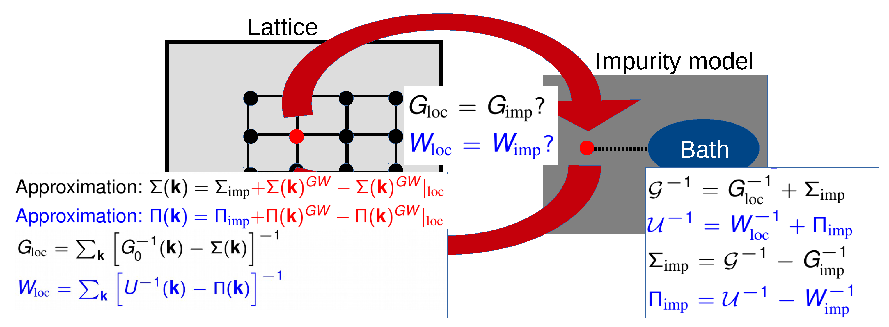
3.1. G W +EDMFT

To overcome the fundamental difficulties of LDA+DMFT, a new approach that combines the G W method and DMFT was introduced fifteen years ago [24]. The physical idea behind this approach is to assign DMFT to account for the strong onsite correlations and to let the G W method take care of the off-site long-range correlations. The long-range correlations are expected to be weaker than the onsite ones so that a perturbative approach in the form of the GWA is expected to be sufficient. From the GWA point of view, the approach is equivalent to including onsite vertex correction via DMFT. Alternatively, from the point of view of DMFT, the approach is an attempt to include non-local self-energy neglected in DMFT. Both of these methods are based on Green’s function technique, which allows for a precise removal of the double-counting term.
The combination of G W and DMFT requires an extension of the latter into the so-called extended DMFT (EDMFT) [71,72,73,74] in which the self-consistency requirement is not only imposed on the impurity Green’s function, but also on the impurity screened interaction. Unlike in the original DMFT, the self-consistency requirement in EDMFT encompasses both the one-particle correlation function (the Green’s function) and the two-particle correlation function (the screened interaction or the density-density response function):
G i m p = G l o c ,
W i m p = W l o c .
This extension is rather general since one could imagine including higher-order or other type of correlation functions in the self-consistency requirement in a systematic manner. Thus, for example, a self-consistency on the impurity three-point vertex function leads to the so-called TRILEX scheme [75,76]. An important aspect in EDMFT is the possibility of having a retarded, or, equivalently, energy-dependent interaction. In the EDMFT, the impurity action is given by
S = 0 β d τ d τ a b σ c a σ ( τ ) [ δ ( τ τ ) τ G a b σ 1 ( τ τ ) ] c b σ ( τ ) + 1 2 0 β d τ d τ σ σ a b c d U a b d c ( τ τ ) c a σ ( τ ) c b σ ( τ ) c c σ ( τ ) c d σ ( τ ) ,
which, with the Fermionic Weiss field G and the effective impurity interaction U as input, is used to solve the impurity problem yielding the impurity Green’s function G i m p and charge susceptibility χ i m p . It is not until rather recently that a method for solving the impurity problem with a retarded interaction is available [65,66,67,68,69]. From the charge susceptibility, we obtain the impurity screened interaction
W i m p = U U χ i m p U .
The impurity self-energy Σ i m p and the impurity polarization P i m p are then extracted from the following Dyson equations:
Σ i m p = G 1 G i m p 1 ,
P i m p = U 1 W i m p 1 .
These in turn are used to compute the local Green’s function and screened interaction:
G l o c = k [ G 0 1 ( k ) Σ i m p ] 1 ,
W l o c = k [ 1 v ( k ) P i m p ] 1 v ( k ) .
Here, the EDMFT approximation has been used in which the k -dependent self-energy and polarization are approximated by the corresponding local impurity quantities. At this stage, we check the self-consistency condition, i.e., whether G i m p = G l o c and W i m p = W l o c . If this is not fulfilled, the Weiss field G and the effective impurity interaction U are updated as follows:
G 1 = G l o c 1 + Σ i m p ,
U 1 = W l o c 1 + P i m p ,
and the iteration is continued until the self-consistency condition is fulfilled.
In EDMFT, the self-energy and polarization are assumed to be local. We now go over to G W +EDMFT by including a non-local self-energy and polarization within the GWA. This would be rather straightforward to do were it simply a matter of adding the non-local components of the G W self-energy and polarization to the corresponding impurity quantities in one shot. We would, however, like to construct a self-consistent scheme in which the non-local contributions from G W affect the local contributions from EDMFT and vice versa. This can be achieved by replacing Σ i m p and P i m p in Equations (57) and (58) by
Σ G W + D M F T ( k ) = Σ G W ( k ) + Σ E D M F T k Σ G W ( k ) ,
P G W + D M F T ( k ) = P G W ( k ) + P E D M F T k P G W ( k ) ,
where the last term in each of the above equations is the local component of the G W contribution, which when subtracted removes the double-counting. In position representation, Σ G W and P G W are given respectively in Equations (21) and (33). For each k -point, Σ G W ( k ) and P G W ( k ) are matrices in some Bloch basis. The full lattice Green’s function needed to compute Σ G W and P G W is obtained from the Dyson equation
G 1 ( k ) = G H 1 ( k ) Σ G W + D M F T ( k ) ,
where G H is the Hartree Green’s function that can be extracted from the Kohn–Sham DFT Green’s function by removing the exchange-correlation potential V x c :
G H 1 = G K S 1 + V x c .
In Figure 4, we show the relationship between DMFT, EDMFT and G W +EDMFT.

3.1.1. Functional Approach

It is possible to formulate the G W +EDMFT scheme using the functional approach [24]. The starting point is the generalized free-energy functional in which in addition to the Green’s function, the screened interaction is added as a basic variable. A particular choice of the free-energy functional has the form [77]
Γ [ G , W ] = Tr [ ln G ] Tr [ ( G H 1 G 1 ) G ] 1 2 Tr [ ln W ] + 1 2 Tr [ ( v 1 W 1 ) W ] + Ψ [ G , W ] ,
which is a generalization of the original Luttinger–Ward functional [78]
Γ L W [ G ] = Tr [ ln G ] Tr [ Σ ( G ) G ] + Φ [ G ] .
The Psi-functional Ψ [ G , W ] contains the effects of exchange and correlation and the self-energy and polarization are obtained from functional derivatives
Σ = δ Ψ δ G , P = 2 δ Ψ δ W .
Within the GWA, Ψ is given by
Ψ G W = 1 2 Tr ( G W G ) ,
whereas the corresponding quantity in EDMFT is formally written as
Ψ E D M F T = Ψ [ G l o c , W l o c ] .
The G W +EDMFT Psi-functional is then
Ψ G W + E D M F T [ G , W ] = Ψ G W + Ψ E D M F T Ψ l o c G W = 1 2 Tr ( G W G ) + Ψ [ G l o c , W l o c ] + 1 2 Tr ( G l o c W l o c G l o c ) ,
where the last term is the double-counting term to remove the local G W contribution already included in Ψ E D M F T . The functional approach has the merit that it obeys conservation laws in the sense of Baym–Kadanoff, i.e., when the self-energy is derivable from a functional, in our case, it is derivable from Ψ [ G , W ] . The stationary requirement on Γ [ G , W ] with respect to G and W yields the Dyson equations:
δ Γ δ G = 0 G 1 = G H 1 Σ ,
δ Γ δ W = 0 W 1 = v 1 P .
The free-energy functional can also be derived using the action formalism starting from the partition function in the grand canonical ensemble for interacting electrons moving in the crystal potential V c , [24,73]
Z = D [ ψ ψ ] exp ( S [ ψ , ψ ] ) ,
where the action S is given by
S [ ψ , ψ ] = d x ψ ( x ) τ 2 2 + V c ( x ) ψ ( x ) 1 2 d x d x ψ ( x ) ψ ( x ) v ( x x ) ψ ( x ) ψ ( x ) .
Decoupling the electron–electron interaction term using the Hubbard–Stratonovic transformation reduces the interaction into a one-particle term at the cost of having an additional bosonic field ϕ ,
S [ ϕ , ψ , ψ ] = d x ψ ( x ) τ 2 2 + V H c ( x ) ψ ( x ) 1 2 d x d x ϕ ( x ) v 1 ( x x ) ϕ ( x ) i α d x ϕ ( x ) ψ ( x ) ψ ( x ) .
Here, V H c is the sum of the Hartree and crystal potentials and α is a coupling constant set to unity for the physical case. We now apply probing fields that couple to the Fermionic and bosonic propagators and the action becomes
S [ ψ , ψ , J f , J b ] = S [ ϕ , ψ , ψ ] d x d x ψ ( x ) J f ( x , x ) ψ ( x ) 1 2 d x d x ϕ ( x ) J b ( x , x ) ϕ ( x ) .
The free energy is
Ω ( J f , J b ) = ln Z ( J f , J b )
from which the Fermionic propagator G ( x , y ) and bosonic propagator W ( x , y ) can be derived:
G ( x , y ) = Ω J f = T ψ ( x ) ψ ( y ) ,
W ( x , y ) = 2 Ω J b = T ψ ( x ) ψ ( y ) .
The free-energy functional is then obtained as a double Legendre transform of Ω :
Γ [ G , W ] = Ω ( J f , J b ) J f G 1 2 J b W .
The Psi-functional in this formulation is given by
Ψ [ G , W ] = 0 1 d α d x ϕ ( x ) ψ ( x ) ψ ( x ) .

3.2. Multitier Self-Consistent G W +EDMFT

The G W +EDMFT formulation presented in the previous section is rather general, but, in practice, EDMFT is applied to a certain subspace of the full Hilbert space typically corresponding to a partially filled narrow band, whereas the GWA is usually applied to the full Hilbert space. It is natural to divide the Hilbert space into a subspace corresponding to the partially filled narrow band (correlated band) and the rest. G W +EDMFT is then applied within the correlated band, whereas the G W self-energy is active in the rest of the Hilbert space. In many materials, however, there may be other bands in the vicinity of the correlated band which hybridize strongly with the correlated band and therefore should be included in the G W +EDMFT calculation, although they do not need to be treated explicitly within the impurity problem. We refer to these bands as intermediate subspace.
Our goal is to perform self-consistent G W +EDMFT calculations, which would eliminate many ambiguities associated with non-self-consistent or partially self-consistent calculations. For example, in non-self-consistent calculations, the double-counting correction is not unique, whereas, in self-consistent calculations, it is uniquely defined. On the other hand, a self-consistent calculation over the complete Hilbert space is physically inadvisable. The reason for this is based on the knowledge that a fully self-consistent G W calculation is expected to yield poor one-particle excitation spectra, as demonstrated in the case of the electron gas [59]. The renormalization of the Green’s function in the self-consistent cycle leads to a reduction of the quasiparticle weight and a transfer of spectral weight to a higher energy region, which in turn weakens screening resulting in a stronger W. We therefore expect a widening of the bandwidth compared to a one-shot G W result, opposite to what experimental data suggest. Moreover, the plasmon excitation appearing in the spectral function is washed out in a self-consistent G W calculation, contrary to experiment [59]. These undesirable effects of self-consistency within the GWA would remain if we were to perform a self-consistent G W +EDMFT calculation over the whole Hilbert space since the vertex corrections furnished by EDMFT are confined to a limited subspace corresponding to the correlated band. In other words, nothing counteracts the detrimental effects of self-consistent G W outside the correlated subspace.
We therefore have in general three subspaces:
  • Subspace 1: The correlated subspace in which self-consistent GW + EDMFT is applied.
  • Subspace 2: The intermediate subspace in which self-consistent GW is active.
  • Subspace 3: The remaining subspace in which a one-shot GW is active.
For example, in the case of transition metal oxides such as NiO, the 3 d band would be treated as the correlated band, whereas the oxygen 2 p band would correspond to the intermediate subspace. In some transitional metal oxide such as SrVO 3 described later, the hybridization between the 3 d and 2 p orbital is much weaker, so it is reasonable to treat the 2 p orbitals as part of the remaining subspace without the need for an intermediate subspace.
This general consideration leads to the idea of multitier self-consistent G W +EDMFT [38,39]. Note that the tiers indicate the theoretical level and they are not the same as the subspaces. In the first step, we perform a one-shot G W calculation over the entire Hilbert space, starting from a non-interacting Green’s function constructed from the LDA band structure, as commonly done. However, we keep the component on this one-shot G W self-energy Σ = i G 0 W 0 only on subspace 3:
Tier III : Σ I I I = Σ G 0 W 0 1 + 2 + 3 Σ G 0 W 0 1 + 2 ,
where the superscripts on the right side of the equation indicate the subspaces. We then perform a fully self-consistent G W +EDMFT calculation in the intermediate and correlated subspaces. To compute the effective electron–electron retarded interaction within the intermediate and correlated subspaces (1 + 2), we use the cRPA method. In Tier II, we remove the local G W self-energy contribution on the impurity site(s) (the double-counting term):
Tier II : Σ I I = Σ G W 1 + 2 Σ G W 1 , l o c .
Finally, in Tier I, we compute the EDMFT self-energy of the impurity problem:
Tier I : Σ I = Σ E D M F T .
Thus, in Tier II, the non-local G W contribution is retained, whereas, in Tier I, the self-energy is equal to the impurity self-energy from EDMFT. Once the self-energy in each tier is obtained, the full Green’s function is given by
G 1 ( k ) = G H 1 ( k ) Σ I I I ( k ) Σ I I ( k ) Σ I .
Similar equation for the screened interaction in terms of the polarization on the different tiers applies, which takes into account the non-local screening at the RPA level and the onsite vertex corrections from EDMFT. For a detailed description of the multitier approach, see Ref. [39].

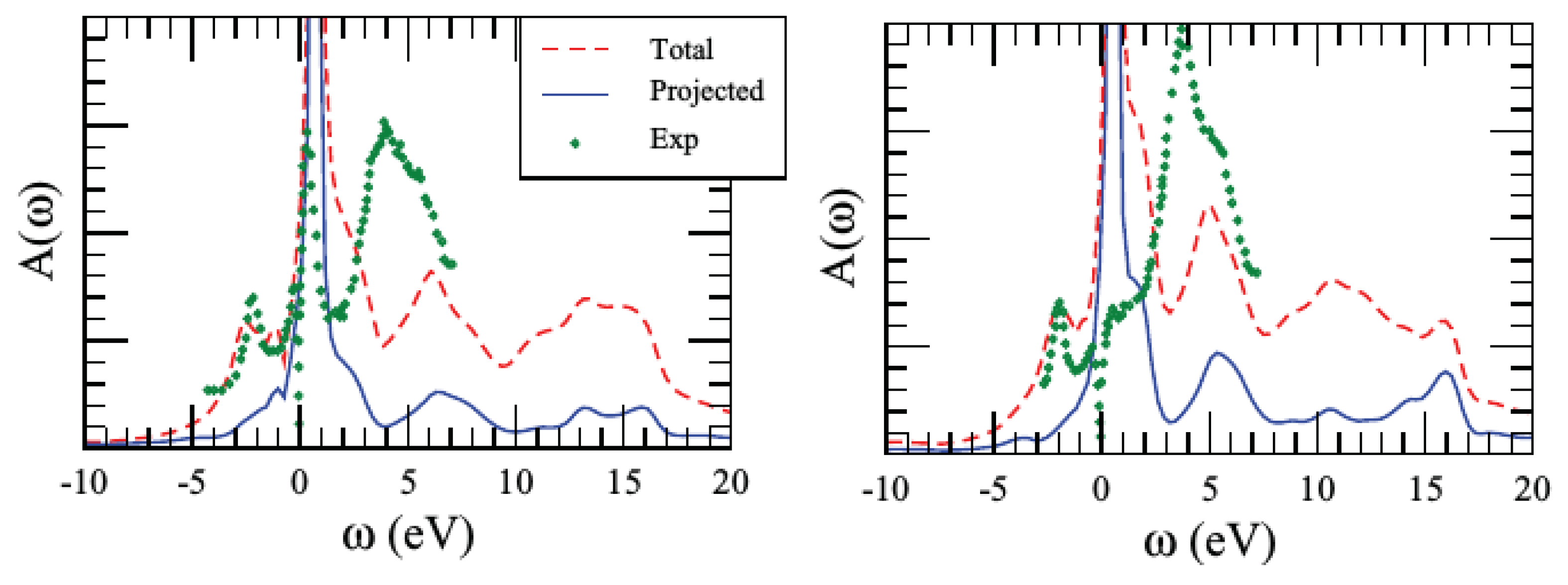
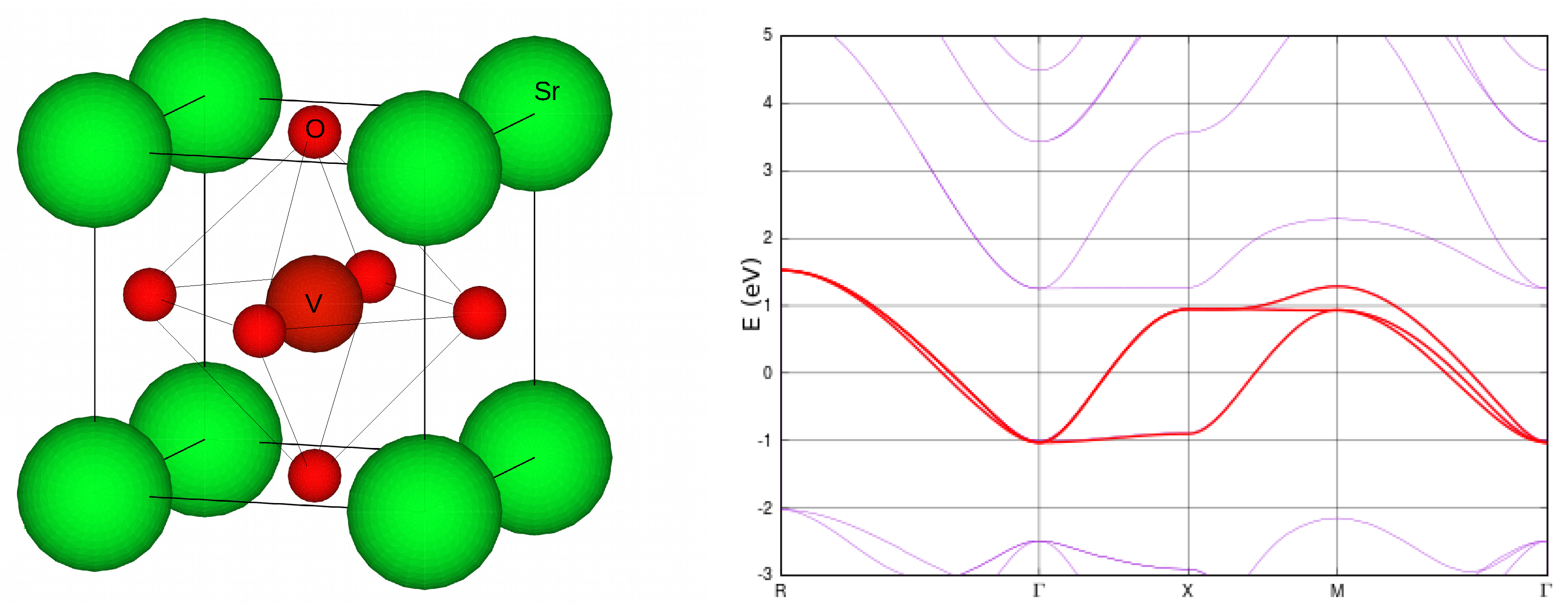
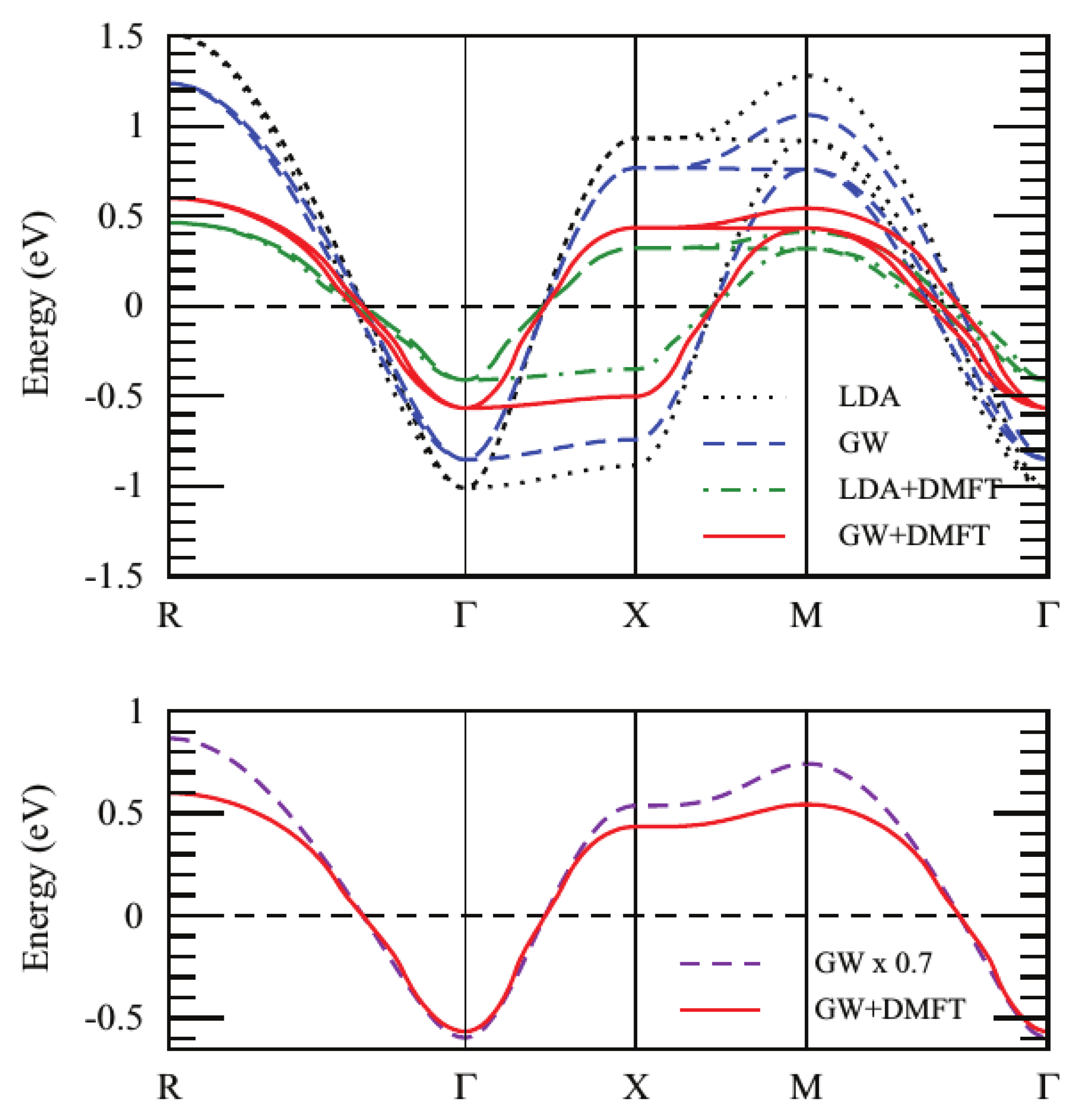
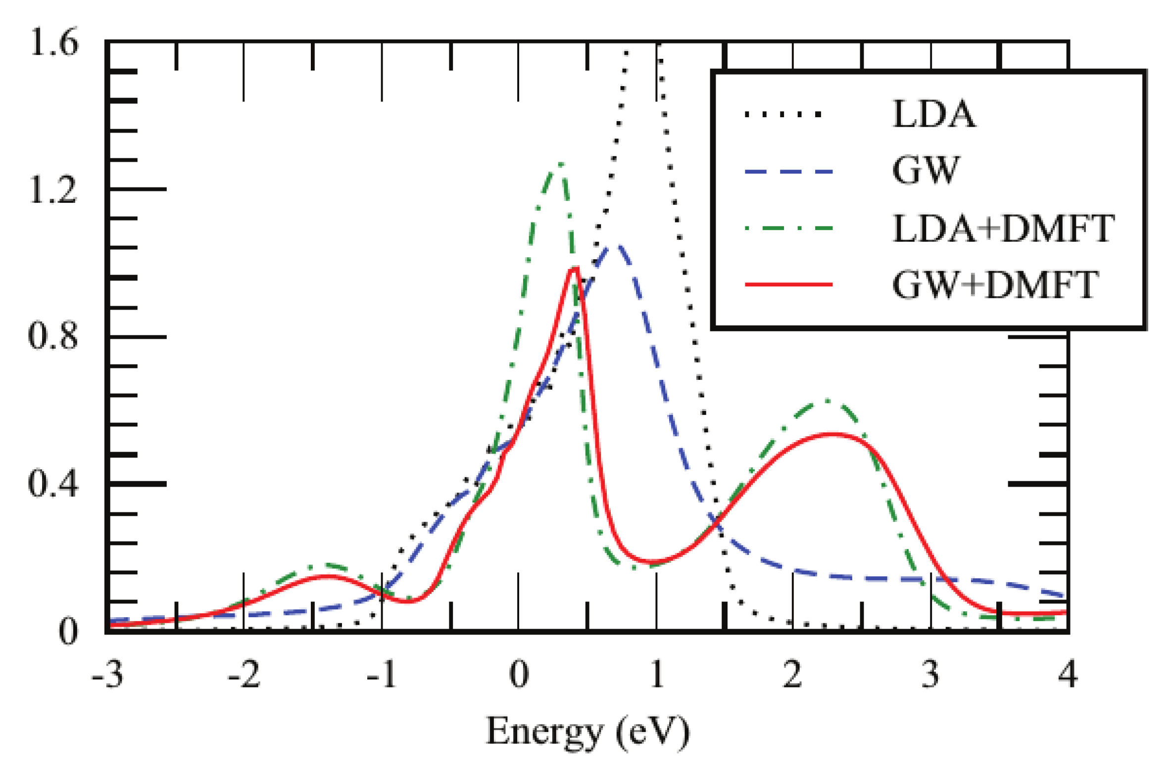
3.3. Illustrative Example: SrVO 3

The cubic perovskite SrVO 3 , which is 3 d 1 system and has been regarded as a paradigm of strongly correlated metals, provides an illustrative example for the application of G W +EDMFT. Therefore, we will use this as our main example to compare the different implementations combining G W -approximation with DMFT.
SrVO 3 cystallizes in a cubic perovskite structure with the vanadium atom centred in an octahedral cage between the oxygen atoms (left panel of Figure 5). Due to the crystal field, the 3 d states of the V atom splits into the t 2 g and e g components. Within the LDA, the t 2 g states form a narrow isolated conduction band occupied with one electron/unit cell, whereas the e g states are unoccupied (right panel of Figure 5). Experimentally, the material exhibits a renormalized quasiparticle peak in between a weak, broad satellite feature centered around −1.5 eV [79,80,81,82,83] and more pronounced upper satellite feature at around 3 eV [79]. The bottom of the t 2 g -band is located around −0.7 eV [80,83] and the effective mass enhancement compared to the LDA is approximately 2 [84], which also agrees with estimations from the specific heat coefficient [85].
Within the GWA, the bandwidth of the t 2 g -bands is 2.1 eV, which corresponds to an effective mass enhancement of approximately 1.2 [38,86,87]. Hence, the correlations included in the GWA are not enough to account for the band renormalization observed experimentally. On the other hand, a strong plasmonic mode originating from transitions within the t 2 g subspace gives rise to a weak satellite feature in the occupied region at an energy around −2 eV in rough agreement with the experimental data [87]. In the occupied region, a plasmon satellite appears at around 3.5 eV, which is corrected to 3 eV using the cumulant expansion [88,89], also in good agreement with experiment [87] (The cumulant calculations in Ref. [87] were based on quasiparticle self-consistent G W -calculations.).
Although G W -based methods seem to be able to describe the satellites as plasmons traditionally the satellite features are explained as Hubbard bands since they appear in LDA+DMFT calculations with a static U (See e.g., [83,90,91,92]), which do not allow for long-range charge fluctuations responsible for plasmon excitations. While LDA+DMFT provides a better description of the lower satellite, the position of the upper satellite is too close to the Fermi energy, even when the effective interaction for the impurity problem is adjusted to give the correct band renormalization. In LDA+DMFT with ab initio interaction parameters from cRPA, the band renormalization is too big (corresponding to an effective mass enhancement of approximately 2.9) and the upper satellite feature is centered around 2.4 eV.
Before we discuss the results from the fully self-consistent multitier G W +EDMFT presented above, we will present some simplified implementations and what we can learn from them.

3.3.1. One-Shot GW+DMFT

The simplest way to combine the GWA with DMFT is to combine the two methods on the one-shot level. That is, combine a one-shot G W calculation with DMFT. The main advantage with this is that it is simple since it is possible to make use of existing electronic structure codes with additional pre- or post-processing tools. However, one major drawback is that the result depends on how the double counting is subtracted.
In Ref. [86], a one-shot G W calculation was first performed in the full Hilbert space. This calculation was then combined with a separate LDA+DMFT calculation restricted to the t 2 g -subspace using a dynamically screened interaction U ( ω ) computed within cRPA. The full self-energy is then given by:
Σ ^ ( ω ) = k n n | ψ k n Σ n n G W ( k , ω ) ψ k n | + m m | ϕ m Σ m m imp ( ω ) Σ m m DC ( ω ) ϕ m | ,
where { ψ k n } are the LDA eigenstates and { ϕ m } are localized Wannier orbitals, in this case constructed from the t 2 g states of the Vanadium atom. The double counting term is given by the local G W selfenergy with all internal sums restricted to the t 2 g subspace:
Σ m m D C ( ω ) = i m 1 m 2 t 2 g 1 2 π d ω G m 1 m 2 loc ( ω + ω ) W m m 1 , m m 2 loc ( ω ) ,
where
W m m 1 , m m 2 loc = d 3 r d 3 r φ m * ( r ) φ m 1 ( r ) W ( r , r ) φ m ( r ) φ m 2 * ( r ) .
The orbitals φ m are usually chosen to the maximally localized Wannier orbitals [93,94,95,96].
It should be noted that W loc has to be evaluated using the local interaction of the impurity problem and the local polarization, and is thereby different from the local projection of the full W,
W loc ( ω ) = [ 1 U loc ( ω ) P loc ( ω ) ] 1 U loc ( ω ) .
Compared to LDA+DMFT, the non-local contribution from the GWA widens the quasiparticle band and slightly lowers the weight of the satellites (Figure 6 and Figure 7). However, the position of the satellites is determined by the impurity problem; therefore, the satellites are interpreted as upper and lower Hubbard bands [86]. This is a generic feature of any method that does not include a self-consistent feedback of the non-local screening on the effective impurity interaction. In these cases, the non-local self-energy will only contribute with an additional dispersion of the satellite features, but cannot change the physical interpretation of the satellites as Hubbard bands. The local vertex corrections from DMFT yields a deviation from the linear behavior of the self-energy for low energies, which yields a kink structure in the dispersion as can be seen in the lower panel of Figure 6. The quasiparticle bandwidth agrees well with the experimental estimations as well as the position of the lower satellite feature. However, similar to the LDA+DMFT results, the upper satellite is still too close to the quasiparticle peak.
In the implementation described above, there is no feedback from the non-local self-energy on the impurity problem. A way to overcome this deficiency is to account for the non-local self-energy at each step in the DMFT self-consistency cycle. That is, in each step of the DMFT cycle the local lattice Green’s function is computed as:
G loc 1 ( ω ) = k H k LDA + V k x c Σ k ( ω ) ,
where Σ k ( ω ) is defined in Equation (83) and all quantities are projected onto the DMFT ( t 2 g ) subspace. Since the local Green’s function enters the equation of the impurity Weiss field G in Equation (59), the effective bare propagator of the impurity includes the effect of the non-local self-energy. This scheme was implemented in Refs. [26,27]. The effect of the non-local self-energy is dramatic. While the occupied part of the spectra is similar to the previous scheme, the unoccupied part is widened substantially, and, at the X-point, the x y / x z states are located at 0.9 eV, which is the same energy as in LDA. This means that the quasiparticle renormalization for these states are even weaker in the combined G W +DMFT calculations than in one-shot G W . For this reason, the upper satellite is absorbed in the quasiparticle dispersion and the peak in the unoccupied region in the BIS-spectra is explained as originating from the e g -states rather than as a t 2 g -satellite.
Further simplifications, based on using the G W quasiparticle band structure [25,27,86], screened exchange approximation [28] as well as the G W quasiparticle self-consistent band structure [29] rather than the full frequency-dependent non-local self-energy have also been investigated and shown to give physically reasonable results. However, we will not discuss these simplifications further in this work.

3.4. Effect of Self-Consistency: Multitier G W +EDMFT

Within the Multitier G W +EDMFT method [38,39], it is natural to use the narrow t 2 g bands as both the correlated and intermediate subspace. Thus, within the t 2 g subspace, the method reduces to a self-consistent G W +EDMFT method while the contributions from outside this subspace is included at the one-shot G W level. Contrary to the simplified implementations discussed above, the multitier approach includes the self-consistent feedback from the non-local self-energy and screening on the impurity problem and also the feedback from the impurity problem on the lattice quantities. This allows us to explore a number of interesting questions that cannot be addressed with the simplified schemes discussed above:
  • Are the local vertex corrections from DMFT sufficient to counteract the detrimental effects of self-consistent G W ?
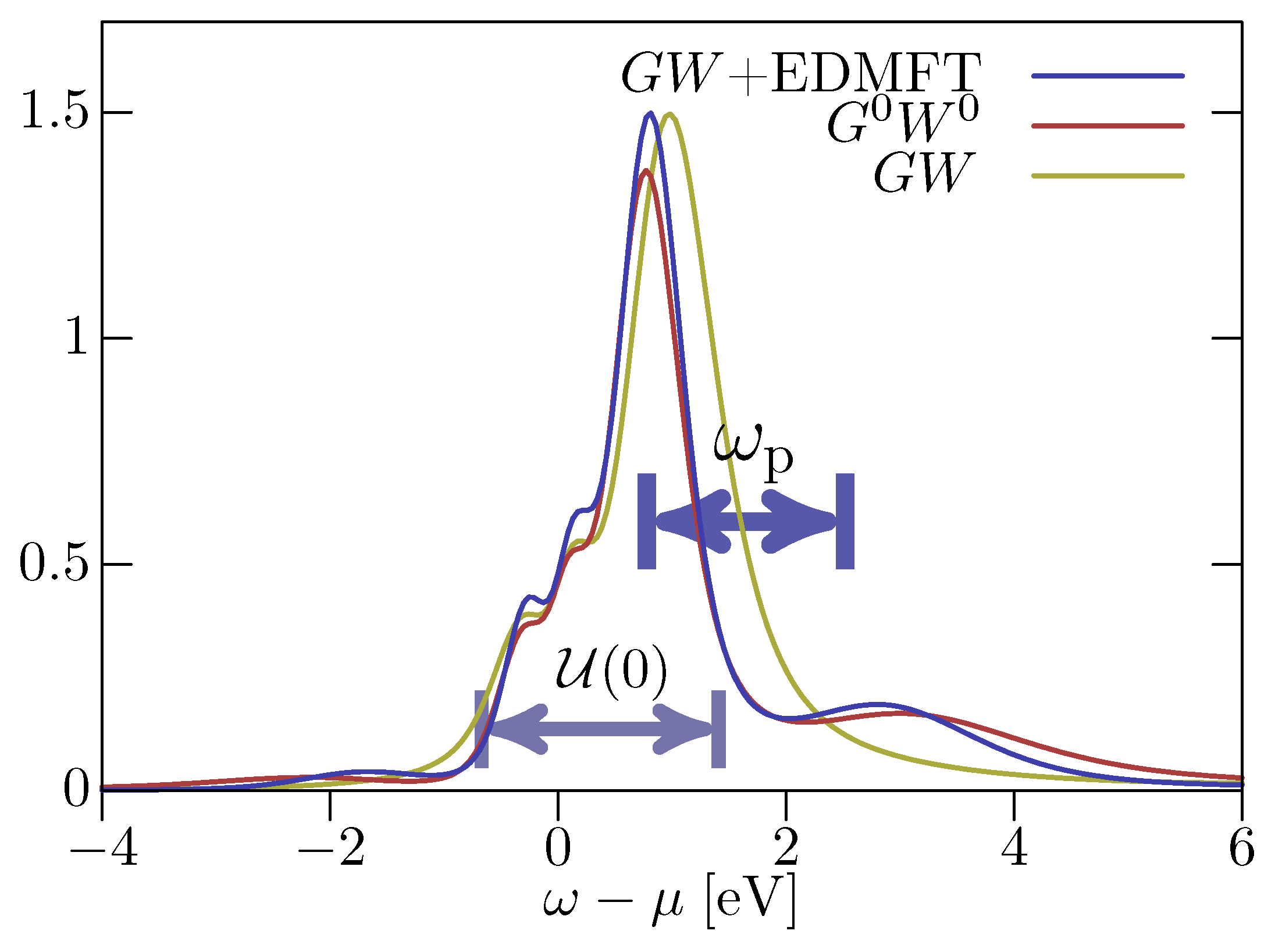
  • What is the role of the long-range screening?
  • What is the nature of the satellites in SrVO 3 ? Are they plasmons as indicated by the G W calculations and the cumulant expansion or are they Hubbard bands as DMFT-based calculations suggest?
In Figure 8, the partial t 2 g spectral functions of SrVO 3 within one-shot G W , self-consistent G W and G W +EDMFT are compared [38]. The one-shot G W results agrees with Ref. [87] and exhibits a renormalized quasiparticle peak in between an upper and lower plasmon satellite. In self-consistent G W , on the other hand, the quasiparticle is widened and the satellites are flushed out. This behavior agrees with the results for the electron gas [59], and indicates that sc G W is not a good approximation also for more strongly correlated solids. The local vertex corrections from EDMFT in the full G W +EDMFT calculations restores the satellites and narrows quasiparticle width. Compared to one-shot G W , the satellites are pulled closer to the quasiparticle, in agreement with the experimental data. To understand the origin of the satellite features, we investigate the fully screened interaction W (Figure 9). Both one-shot G W and G W +EDMFT exhibit clear subplasmonic modes from within the t 2 g -subspace. It is interesting to note that the plasmon energy, ω p , is slightly smaller in the full calculations compared to one-shot G W . This difference originates from the local vertex corrections to the polarization in G W +EDMFT. This also offers an explanation of why the cumulant expansion calculations in Ref. [87] overestimates the energy of the lower satellite. In sc G W , the plasmon is almost entirely flushed out, which also explains the absence of any clear satellite features in the spectral function.
To answer the fundamental question about the nature of the satellites, we have to compare the position of the satellite features with the plasma energy as well as the static impurity interaction. If the satellites are Hubbard bands, they should be separated by roughly the static value of the interaction ( U ( ω = 0 ) ), while, if they are of plasmonic origin, they should appear at roughly one plasmon energy below or above the quasiparticle peak. From Figure 8, it is therefore clear that the satellites should be interpreted as plasmons rather than Hubbard bands. This interpretation is supported by another material, SrMoO 3 , a 3 d 2 system but with a similar electronic structure to SrVO 3 , which has a satellite feature below the quasiparticle peak that is not reproduced within the LDA+DMFT scheme within a physically reasonable range of U [97] but reproduced within the G W +EDMFT scheme [39].
In Figure 10, the k -resolved spectral functions from one-shot G W , LDA+DMFT and G W +EDMFT are compared. The quasiparticle bandwidth in the full G W +EDMFT calculations is strikingly similar to one-shot G W and slightly larger than what the experimental data suggests, which indicates the need to go beyond the GWA also for the non-local terms.
In order to investigate the multitier approach further and understand in which regimes the G W +EDMFT method is applicable, the method was applied to stretched sodium in Ref. [39]. Sodium is an electron-gas like metal with weak correlations. By artificially increasing the lattice constant, it is possible to successively increase the degree of local correlations and thereby test the method on realistic systems with different degrees of correlation. The low-energy band structure of sodium contains a broad s-like conduction band entangled with unoccupied p-like bands. To include all low-energy physics in the self-consistency cycle, the intermediate subspace was defined as the full s + p -subspace (green + black bands in Figure 11), while the correlated subspace was restricted to the s-like component (green components in Figure 11).
In Figure 12, the effective impurity interaction is compared to the bare (cRPA) interaction for three different cases. Here, the effect of the long-range screening is unraveled. While the bare Coulomb interaction follows the counter-intuitive trend of decreasing interaction with increasing lattice constant, the effective impurity interaction follows the physically expected trend; that is, it increases as the atoms are pulled apart. Hence, in this case, a proper treatment of the long-range screening is essential. However, looking at the spectral functions in Figure 13, one can see that, for electron-gas like materials (that is for the original lattice constant, a 0 ), the non-local diagrams included in G W +EDMFT are not sufficient and the method gives similar results as self-consistent G W with a wide quasiparticle peak and flushed out satellite structures. As the lattice constant is increased, the local correlations become increasingly important and the satellite structures are restored. At a separation of 1.6 a 0 , the local correlations completely dominate and the material becomes a Mott–Hubbard insulator.

3.5. Different Levels of Self-Consistency

The original combination of G W and dynamical mean-field theory [24] was derived from the Ψ -functional [77] and hence contains a self-consistency on both the one-particle (G) and two-particle (W) level. An alternative formulation was explored in Ref. [98] for the hydrogen dimer. In this work, a G W +DMFT formulation was derived from the Baym–Kadanoff (BK) functional [99,100] instead:
Γ [ G ] = Tr ln G Tr ( ( G 0 1 G 1 ) G ) + Φ v [ G ] .
Here, Φ v [ G ] contains the effects of exchange and correlations and the functional derivative of Φ with respect to the Green’s function yields the self-energy:
δ Φ v [ G ] δ G = Σ .
The basic idea is that the bosonic self-consistency can be avoided with this formalism. However, this also means that the formalism neglects the effect of non-local screening on the effective impurity interaction, which implies that, similar to LDA+DMFT, the strength of the effective impurity interaction does not come out naturally from the formalism but has to be considered an independent parameter. In addition, as will turn out to be important, the double-counting term between the G W and DMFT self-energies ( Σ DC BK ) is different than in the full formulation:
Σ i k DC BK = G j l loc ( τ ) W i j k l G W imp ( τ ) ,
W G W imp = 1 U Π loc 1 U ,
Π m m n n loc ( τ ) = G m n loc ( τ ) G n m loc ( τ ) ,
where U is the chosen impurity interaction, which in this case is fixed, G loc the local projection of the Green’s function and implicit summation over repeated indexes is assumed. For the hydrogen dimer, it was shown that this double counting leads to non-causal hybridizations due to the non-causality of the difference
Σ G W loc Σ DC BK ,
where Σ G W loc is the local projection of the G W self-energy [98]. In the complete Ψ -derivable theory, however, this problem is not expected since the two terms in Equation (93) exactly cancel if the DMFT and G W subspaces are the same or, in the case where the DMFT subspace is smaller than the G W -subspace, reduces to
Σ G W loc Σ DC i k = j , l r G j l loc W i j k l loc ,
which is causal by construction. Here, r is the difference between the full Hilbert space and the DMFT subspace [39].
On the other hand, it was shown in Ref. [39] that the complete Ψ -derivable theory has different causality problems, namely that the effective impurity interaction can become noncausal in certain parameter regimes. By using a dimer model that can be solved exactly, it was also shown that this is not a unique property of G W +EDMFT.
Any ( Ψ -derivable) theory that maps the lattice problem to a local impurity problem with the self-consistency equations
G loc ( i ν n ) = G imp ( i ν n ) ,
W loc ( i ω n ) = W imp ( i ω n ) ,
is expected to experience noncausal impurity interactions in certain parameter regimes. However, all physical observables remain causal. Since the effective impurity interaction is an auxiliary quantity, the non-causality is not a problem per se, although it can pose numerical difficulties in certain cases.

4. Conclusions

Substantial progress has been achieved in the last decade in describing the electronic structure of correlated materials from first principles. This progress owes its success to the combination of first-principles approaches and model-Hamiltonian-based many-body approaches. Two parallel developments in many-body approaches have fueled the progress: there is an approach using the traditional many-body perturbation theory (diagrammatic method) based on the Green’s function technique, which has as its starting point a realistic band structure usually obtained from the LDA, and there is another approach that uses a model Hamiltonian as its starting point. The first approach has the great advantage of avoiding the use of adjustable parameters and including the details of the electronic structure, which are often important in determining many physical properties, but it has the disadvantage of having to deal with a large number of degrees of freedom, which makes it difficult to go beyond the GWA (RPA) [21]. Although it is possible to include more diagrams beyond the RPA, progress has been rather limited due to the numerical complexity as well as theoretical difficulties in selecting which classes of diagrams are to be summed. Opposite to the first approach, the second approach has the disadvantage that the model usually contains parameters and therefore the starting electronic structure is not always realistic, lacking the full details of the LDA. On the other hand, it has the advantage of having a relatively small number of degrees of freedom in the model Hamiltonian that allows for a more sophisticated many-body treatment of the problem. Indeed, with the arrival of DMFT [14,15,16] it is possible to solve the many-body problem within an impurity model exactly by numerical means. The seminal idea of including the Hubbard U term on top of the LDA Hamiltonian, yielding the LDA+U scheme [7,12,13] evolved into the LDA+DMFT scheme [17,18,19,20] in which the LDA+U Hamiltonian is solved using the more sophisticated DMFT method rather than the Hartree–Fock approximation. Two fundamental problems in the LDA+DMFT scheme arise from the difficulty in removing the double-counting correction and the assumption that the self-energy is local (onsite). In early calculations, the Hubbard U was often treated as an adjustable parameter, but it is now possible to make a good estimate of it using the cLDA [42,43] or cRPA [63] methods. A natural step beyond LDA+DMFT is to combine the GWA and DMFT leading to the GW+EDMFT scheme [24]. Since both are Green’s function approaches, the double-counting term can be accounted for precisely and the GWA provides a non-local self-energy missing in the DMFT method. Alternatively, from the point of view of the GWA, the DMFT provides local or onsite vertex corrections beyond the RPA, thus offering a theoretically ideal scheme for treating correlated materials from first principles.
To gauge the performance of the G W +EDMFT scheme, we have primarily considered the much studied cubic perovskite SrVO 3 , which is a 3 d 1 system. Experimentally, the spectral function of SrVO 3 is characterized by the presence of a quasiparticle peak around the Fermi level sandwiched by two satellite features, which have been interpreted as lower and upper Hubbard bands. LDA+DMFT calculations [83,90,91,92] did indeed reproduce such features and so did the first few G W +EDMFT calculations [26,27,86]. The latter calculations, however, are rather similar to the former in that, instead of starting with the LDA band structure, one starts with a one-shot G W band structure, although they have the advantage of having a more accurate G W band structure and a more rigorous removal of the double-counting term. An important ingredient missing in these calculations is self-consistency. Self-consistent G W +EDMFT calculations show that the feedback from long-range screening can have a substantial effect in reducing the strength of the impurity U so that its static value is too small to account for the energy separation between the lower and upper satellites. Careful analysis reveals that the satellite features are better understood as long-range charge fluctuations or plasmon excitations [38]. This interpretation is supported by another material SrMoO 3 [39].
Self-consistent G W +EDMFT calculations on stretched sodium exhibit a possible range of validity of the scheme. In the weak correlated regime corresponding to the physical equilibrium lattice constant, the scheme fails to give a proper description of the satellite feature. At larger separation, the scheme appears to give a reasonable account of the electronic structure producing the expected Mott gap at 1.5 the equilibrium lattice constant. This study suggests that long-range vertex corrections become increasingly important as the electrons become more itinerant [39].
Including long-range vertex corrections, which are left out in the G W +EDMFT scheme, should be the next step in going beyond G W +EDMFT. However, before going further, much work needs to be done in investigating the performance of the scheme and there are many applications to interesting materials in which long-range correlations are expected to be important. Transition metals in which the electrons are semi itinerant are interesting systems to study within the scheme. A reliable description of the phase diagram of iron, in particular, poses a long-standing challenge. How the scheme treats the so-called charge transfer insulators, such as the transition metal monoxides (NiO, CoO, FeO, etc.) and the parent compounds of the high-temperature superconductors is highly interesting to know. The screening arising from the relatively wide oxygen p band can bring new unexpected physics when treated self-consistently within the G W +EDMFT scheme. Simplifying the scheme along the direction of multitier G W +EDMFT [39] is a possible route for applications to complex materials with many atoms per unit cell.

Acknowledgments

This work was supported by the Swedish Research Council (VR). Part of the computations was performed on resources provided by the Swedish National Infrastructure for Computing (SNIC) at LUNARC.

Conflicts of Interest

The authors declare no conflict of interest. The founding sponsors had no role in the design of the study; in the collection, analyses, or interpretation of data; in the writing of the manuscript, and in the decision to publish the results.

Appendix A. Construction of a Low-Energy Model

Appendix A.1. Constrained RPA

Constructing an accurate effective low-energy model is a crucial first step in calculating the electronic structure of correlated materials. While the one-particle term in the effective low-energy model can be reliably obtained from DFT within the LDA, the effective electron–electron interaction poses a much more difficult problem. A systematic way of removing the high-energy degrees of freedom and encoding them in the effective interaction is provided by the constrained RPA (cRPA) method [63]. The resulting effective interaction is necessarily energy dependent.
The idea of cRPA is to divide the total polarization of the system into the polarization within the model subspace, which we shall call P d , and the rest of the polarization, which we shall call P r . Accordingly,
P = P d + P r .
The fully screened Coulomb interaction is obtained by solving Equation (35):
W = v + v P W ,
which can be rewritten as follows
W = W r + W r P d W ,
where W r fulfills
W r = v + v P r W r .
It can be readily verified by substituting Equation (A4) into Equation (A3) that Equation (A2) is recovered. The identity in Equation (A3) permits us to interpret W r as the effective interaction among electrons residing in the model subspace or the Hubbard U [63]:
U ( r , r ; ω ) = W r ( r , r ; ω ) .
The reasoning behind this interpretation is that, when this effective interaction is screened further in the model by P d , we obtain the fully screened interaction as evident in Equation (A3). As a consequence of retarded screening effects, the Hubbard U is frequency dependent. The screening effects arising from polarization channels P r are encoded in U as a retarded or energy-dependent screened interaction. In the commonly used Hubbard model with a static U, this retardation effect is not taken into account and it can play an important role in determining the electronic structure of the model. A formal derivation of the Hubbard U from the many-electron Hamiltonian may be found in Ref. [101]. Equation (A4) is exact, but, in practice, we approximate P r = P P d within the RPA.

Appendix A.2. Downfolding the Self-Energy

To improve the one-particle part, we need to include the self-energy contribution from the subspace outside the correlated d subspace. The effective self-energy acting on the d subspace has the general form given by [101]
Σ e f f = Σ d + Σ r d ,
where Σ d is the self-energy within the d subspace and Σ r d describes the influence of the rest of the subspace r on the correlated subspace d. It is to be noted that Σ d is not a projection of the total self-energy onto the d subspace and Σ r d is not simply the matrix element of the self-energy between the d and r subspaces. The Green’s function within the d subspace fulfills the following equation
[ ω h Σ e f f ( ω ) ] G d ( ω ) = 1 ,
where h is the Hartree Hamiltonian.
This general formulation was recently implemented within the GWA [102] in which the resulting Σ e f f is used to construct the quasiparticle band structures of SrVO 3 . A model Hamiltonian for the correlated band is defined with a static interaction obtained within cRPA and the G W self-energy contribution corresponding to this static interaction is then removed from Σ e f f , yielding a model with a one-electron energy dispersion that is void of the self-energy correction within the correlated subspace. The idea is that, when the model is solved using a more sophisticated method such as DMFT, it is not necessary to take into account the double-counting correction, since it is already removed from the model.

References

  1. Hohenberg, P.; Kohn, W. Inhomogeneous Electron Gas. Phys. Rev. 1964, 136, B864–B871. [Google Scholar] [CrossRef]
  2. Kohn, W.; Sham, L.J. Self-Consistent Equations Including Exchange and Correlation Effects. Phys. Rev. 1965, 140, A1133–A1138. [Google Scholar] [CrossRef]
  3. Perdew, J.P.; Burke, K.; Ernzerhof, M. Generalized Gradient Approximation Made Simple. Phys. Rev. Lett. 1996, 77, 3865–3868. [Google Scholar] [CrossRef] [PubMed]
  4. Heyd, J.; Scuseria, G.E.; Ernzerhof, M. Hybrid functionals based on a screened Coulomb potential. J. Chem. Phys. 2003, 118, 8207–8215. [Google Scholar] [CrossRef]
  5. Jones, R.O. Density functional theory: Its origins, rise to prominence, and future. Rev. Mod. Phys. 2015, 87, 897–923. [Google Scholar] [CrossRef]
  6. Aryasetiawan, F.; Gunnarsson, O. The GW method. Rep. Prog. Phys. 1998, 61, 237. [Google Scholar] [CrossRef]
  7. Anisimov, V.I.; Lichtenstein, A.I. LDA+U Method: Screened Coulomb Interaction in the Mean-Field Approximation. In Strong Coulomb Correlations in Electronic Structure Calculations. Beyond the Local Density Approximation; Anisimov, V.I., Ed.; Gordon and Breach: New York, NY, USA, 2001; Volume 1, pp. 97–165. [Google Scholar]
  8. Shen, Z.X.; Dessau, D. Electronic structure and photoemission studies of late transition-metal oxides—Mott insulators and high-temperature superconductors. Phys. Rep. 1995, 253, 1–162. [Google Scholar] [CrossRef]
  9. Lee, P.A.; Nagaosa, N.; Wen, X.G. Doping a Mott insulator: Physics of high-temperature superconductivity. Rev. Mod. Phys. 2006, 78, 17–85. [Google Scholar] [CrossRef]
  10. Bednorz, J.G.; Müller, K.A. Possible highTc superconductivity in the Ba-La-Cu-O system. Z. Für Phys. B Condens. Matter 1986, 64, 189–193. [Google Scholar] [CrossRef]
  11. Ramirez, A.P. Colossal magnetoresistance. J. Phys. Condens. Matter 1997, 9, 8171. [Google Scholar] [CrossRef]
  12. Anisimov, V.I.; Zaanen, J.; Andersen, O.K. Band theory and Mott insulators: Hubbard U instead of Stoner I. Phys. Rev. B 1991, 44, 943–954. [Google Scholar] [CrossRef]
  13. Anisimov, V.I.; Aryasetiawan, F.; Lichtenstein, A.I. First-principles calculations of the electronic structure and spectra of strongly correlated systems: The LDA+U method. J. Phys. Condens. Matter 1997, 9, 767. [Google Scholar] [CrossRef]
  14. Metzner, W.; Vollhardt, D. Correlated Lattice Fermions in d = ∞ Dimensions. Phys. Rev. Lett. 1989, 62, 324–327. [Google Scholar] [CrossRef] [PubMed]
  15. Georges, A.; Kotliar, G. Hubbard model in infinite dimensions. Phys. Rev. B 1992, 45, 6479–6483. [Google Scholar] [CrossRef]
  16. Georges, A.; Kotliar, G.; Krauth, W.; Rozenberg, M.J. Dynamical mean-field theory of strongly correlated fermion systems and the limit of infinite dimensions. Rev. Mod. Phys. 1996, 68, 13–125. [Google Scholar] [CrossRef]
  17. Anisimov, V.I.; Poteryaev, A.I.; Korotin, M.A.; Anokhin, A.O.; Kotliar, G. First-principles calculations of the electronic structure and spectra of strongly correlated systems: dynamical mean-field theory. J. Phys. Condens. Matter 1997, 9, 7359. [Google Scholar] [CrossRef]
  18. Lichtenstein, A.I.; Katsnelson, M.I. Ab initio calculations of quasiparticle band structure in correlated systems: LDA++ approach. Phys. Rev. B 1998, 57, 6884–6895. [Google Scholar] [CrossRef]
  19. Kotliar, G.; Savrasov, S.Y.; Haule, K.; Oudovenko, V.S.; Parcollet, O.; Marianetti, C.A. Electronic structure calculations with dynamical mean-field theory. Rev. Mod. Phys. 2006, 78, 865–951. [Google Scholar] [CrossRef]
  20. Held, K. Electronic structure calculations using dynamical mean field theory. Adv. Phys. 2007, 56, 829–926. [Google Scholar] [CrossRef]
  21. Hedin, L. New Method for Calculating the One-Particle Green’s Function with Application to the Electron-Gas Problem. Phys. Rev. 1965, 139, A796–A823. [Google Scholar] [CrossRef]
  22. Hedin, L. On correlation effects in electron spectroscopies and the GW approximation. J. Phys. Condens. Matter 1999, 11, R489. [Google Scholar] [CrossRef]
  23. Onida, G.; Reining, L.; Rubio, A. Electronic excitations: density-functional versus many-body Green’s-function approaches. Rev. Mod. Phys. 2002, 74, 601–659. [Google Scholar] [CrossRef]
  24. Biermann, S.; Aryasetiawan, F.; Georges, A. First-principles approach to the electronic structure of strongly correlated systems: Combining the GW approximation and dynamical mean-field theory. Phys. Rev. Lett. 2003, 90, 086402. [Google Scholar] [CrossRef] [PubMed]
  25. Taranto, C.; Kaltak, M.; Parragh, N.; Sangiovanni, G.; Kresse, G.; Toschi, A.; Held, K. Comparing quasiparticle GW+DMFT and LDA+DMFT for the test bed material SrVO3. Phys. Rev. B 2013, 88, 165119. [Google Scholar] [CrossRef]
  26. Tomczak, J.M.; Casula, M.; Miyake, T.; Aryasetiawan, F.; Biermann, S. Combined GW and dynamical mean-field theory: Dynamical screening effects in transition metal oxides. EPL (Europhys. Lett.) 2012, 100, 67001. [Google Scholar] [CrossRef]
  27. Tomczak, J.M.; Casula, M.; Miyake, T.; Biermann, S. Asymmetry in band widening and quasiparticle lifetimes in SrVO3: Competition between screened exchange and local correlations from combined GW and dynamical mean-field theory GW+DMFT. Phys. Rev. B 2014, 90, 165138. [Google Scholar] [CrossRef]
  28. Van Roekeghem, A.; Biermann, S. Screened exchange dynamical mean-field theory and its relation to density functional theory: SrVO3 and SrTiO3. EPL (Europhys. Lett.) 2014, 108, 57003. [Google Scholar] [CrossRef]
  29. Choi, S.; Kutepov, A.; Haule, K.; van Schilfgaarde, M.; Kotliar, G. First-principles treatment of Mott insulators: Linearized QSGW+DMFT approach. Npj Quantum Mater. 2016, 1, 16001. [Google Scholar] [CrossRef]
  30. Karlsson, K. Self-consistent GW combined with single-site dynamical mean field theory for a Hubbard model. J. Phys. Condens. Matter 2005, 17, 7573. [Google Scholar] [CrossRef]
  31. Ayral, T.; Werner, P.; Biermann, S. Spectral Properties of Correlated Materials: Local Vertex and Nonlocal Two-Particle Correlations from Combined GW and Dynamical Mean Field Theory. Phys. Rev. Lett. 2012, 109, 226401. [Google Scholar] [CrossRef] [PubMed]
  32. Ayral, T.; Biermann, S.; Werner, P. Screening and nonlocal correlations in the extended Hubbard model from self-consistent combined GW and dynamical mean field theory. Phys. Rev. B 2013, 87, 125149. [Google Scholar] [CrossRef]
  33. Hansmann, P.; Ayral, T.; Vaugier, L.; Werner, P.; Biermann, S. Long-Range Coulomb Interactions in Surface Systems: A First-Principles Description within Self-Consistently Combined GW and Dynamical Mean-Field Theory. Phys. Rev. Lett. 2013, 110, 166401. [Google Scholar] [CrossRef] [PubMed]
  34. Huang, L.; Ayral, T.; Biermann, S.; Werner, P. Extended dynamical mean-field study of the Hubbard model with long-range interactions. Phys. Rev. B 2014, 90, 195114. [Google Scholar] [CrossRef]
  35. Van Loon, E.G.C.P.; Krien, F.; Hafermann, H.; Stepanov, E.A.; Lichtenstein, A.I.; Katsnelson, M.I. Double occupancy in dynamical mean-field theory and the dual boson approach. Phys. Rev. B 2016, 93, 155162. [Google Scholar] [CrossRef] [Green Version]
  36. Stepanov, E.A.; van Loon, E.G.C.P.; Katanin, A.A.; Lichtenstein, A.I.; Katsnelson, M.I.; Rubtsov, A.N. Self-consistent dual boson approach to single-particle and collective excitations in correlated systems. Phys. Rev. B 2016, 93, 045107. [Google Scholar] [CrossRef]
  37. Ayral, T.; Biermann, S.; Werner, P.; Boehnke, L. Influence of Fock exchange in combined many-body perturbation and dynamical mean field theory. Phys. Rev. B 2017, 95, 245130. [Google Scholar] [CrossRef]
  38. Boehnke, L.; Nilsson, F.; Aryasetiawan, F.; Werner, P. When strong correlations become weak: Consistent merging of GW and DMFT. Phys. Rev. B 2016, 94, 201106. [Google Scholar] [CrossRef]
  39. Nilsson, F.; Boehnke, L.; Werner, P.; Aryasetiawan, F. Multitier self-consistent GW+EDMFT. Phys. Rev. Mater. 2017, 1, 043803. [Google Scholar] [CrossRef]
  40. Slater, J.C. A Simplification of the Hartree-Fock Method. Phys. Rev. 1951, 81, 385–390. [Google Scholar] [CrossRef]
  41. Slater, J.C. The History of the Xα Method. In The World of Quantum Chemistry; Daudel, R., Pullman, B., Eds.; D. Reidel Publishing Company: Dordrecht, The Netherlands, 1974; pp. 3–15. [Google Scholar]
  42. Gunnarsson, O.; Andersen, O.K.; Jepsen, O.; Zaanen, J. Density-functional calculation of the parameters in the Anderson model: Application to Mn in CdTe. Phys. Rev. B 1989, 39, 1708–1722. [Google Scholar] [CrossRef]
  43. Cococcioni, M.; de Gironcoli, S. Linear response approach to the calculation of the effective interaction parameters in the LDA+U method. Phys. Rev. B 2005, 71, 035105. [Google Scholar] [CrossRef]
  44. Allen, J.W. Resonant Photoemission of Solids with Strongly Correlated Electrons. In Synchroton Radiation Research, Advances in Surface Interface Science, 1st ed.; Bachrach, R.Z., Ed.; Springer Science+Business Media: New York, NY, USA, 1992; pp. 253–315. [Google Scholar]
  45. Karlsson, K.; Aryasetiawan, F.; Jepsen, O. Method for calculating the electronic structure of correlated materials from a truly first-principles LDA+U scheme. Phys. Rev. B 2010, 81, 245113. [Google Scholar] [CrossRef]
  46. The FLEUR Group. The FLEUR Project. Available online: http://www.flapw.de (accessed on 10 March 2012).
  47. Fetter, A.; Walecka, J. Quantum Theory of Many-Particle Systems; Dover: Mineola/New York, NY, USA, 2003. [Google Scholar]
  48. Aulbur, W.G.; Jönsson, L.; Wilkins, J.W. Quasiparticle Calculations in Solids; Academic Press: Cambridge, MA, USA, 2000; Volume 54, pp. 1–218. [Google Scholar]
  49. Pines, D. Elementary Excitations in Solids; Benjamin: New York, NY, USA, 1963. [Google Scholar]
  50. Zhu, X.; Louie, S.G. Quasiparticle band structure of thirteen semiconductors and insulators. Phys. Rev. B 1991, 43, 14142–14156. [Google Scholar] [CrossRef]
  51. Rohlfing, M.; Krüger, P.; Pollmann, J. Quasiparticle band-structure calculations for C, Si, Ge, GaAs, and SiC using Gaussian-orbital basis sets. Phys. Rev. B 1993, 48, 17791–17805. [Google Scholar] [CrossRef]
  52. Zakharov, O.; Rubio, A.; Blase, X.; Cohen, M.L.; Louie, S.G. Quasiparticle band structures of six II–VI compounds: ZnS, ZnSe, ZnTe, CdS, CdSe, and CdTe. Phys. Rev. B 1994, 50, 10780–10787. [Google Scholar] [CrossRef]
  53. Godby, R.W.; Schlüter, M.; Sham, L.J. Self-energy operators and exchange-correlation potentials in semiconductors. Phys. Rev. B 1988, 37, 10159–10175. [Google Scholar] [CrossRef]
  54. Rubio, A.; Corkill, J.L.; Cohen, M.L.; Shirley, E.L.; Louie, S.G. Quasiparticle band structure of AlN and GaN. Phys. Rev. B 1993, 48, 11810–11816. [Google Scholar] [CrossRef]
  55. Schönberger, U.; Aryasetiawan, F. Bulk and surface electronic structures of MgO. Phys. Rev. B 1995, 52, 8788–8793. [Google Scholar] [CrossRef]
  56. Hellwege, K.H.; Madelung, O. (Eds.) Numerical Data and Functional Relationships in Science and Technology; Landolt-Börnstein, New Series, Group III, Vols. 17a and 22a; Springer: Berlin/Heidelberg, Germany, 1982. [Google Scholar]
  57. Baldini, G.; Bosacchi, B. Optical Properties of Na and Li Halide Crystals at 55 °K. Phys. Status Solidif. 1970, 38, 325–334. [Google Scholar] [CrossRef]
  58. Whited, R.; Flaten, C.J.; Walker, W. Exciton thermoreflectance of MgO and CaO. Solid State Commun. 1973, 13, 1903–1905. [Google Scholar] [CrossRef]
  59. Holm, B.; von Barth, U. Fully self-consistent GW self-energy of the electron gas. Phys. Rev. B 1998, 57, 2108–2117. [Google Scholar] [CrossRef]
  60. Kotani, T.; van Schilfgaarde, M.; Faleev, S.V. Quasiparticle self-consistent GW method: A basis for the independent-particle approximation. Phys. Rev. B 2007, 76, 165106. [Google Scholar] [CrossRef]
  61. Sakuma, R.; Miyake, T.; Aryasetiawan, F. Self-energy and spectral function of Ce within the GW approximation. Phys. Rev. B 2012, 86, 245126. [Google Scholar] [CrossRef]
  62. Hewson, A.C. The Kondo Problem to Heavy Fermions; Cambridge Studies in Magnetism; Cambridge University Press: Cambridge, UK, 1997. [Google Scholar]
  63. Aryasetiawan, F.; Imada, M.; Georges, A.; Kotliar, G.; Biermann, S.; Lichtenstein, A.I. Frequency-dependent local interactions and low-energy effective models from electronic structure calculations. Phys. Rev. B 2004, 70, 195104. [Google Scholar] [CrossRef]
  64. Amadon, B.; Biermann, S.; Georges, A.; Aryasetiawan, F. The α-γ Transition of Cerium Is Entropy Driven. Phys. Rev. Lett. 2006, 96, 066402. [Google Scholar] [CrossRef] [PubMed]
  65. Werner, P.; Comanac, A.; de’ Medici, L.; Troyer, M.; Millis, A.J. Continuous-Time Solver for Quantum Impurity Models. Phys. Rev. Lett. 2006, 97, 076405. [Google Scholar] [CrossRef] [PubMed]
  66. Werner, P.; Millis, A.J. Hybridization expansion impurity solver: General formulation and application to Kondo lattice and two-orbital models. Phys. Rev. B 2006, 74, 155107. [Google Scholar] [CrossRef]
  67. Werner, P.; Millis, A.J. Efficient Dynamical Mean Field Simulation of the Holstein-Hubbard Model. Phys. Rev. Lett. 2007, 99, 146404. [Google Scholar] [CrossRef] [PubMed]
  68. Werner, P.; Millis, A.J. Dynamical Screening in Correlated Electron Materials. Phys. Rev. Lett. 2010, 104, 146401. [Google Scholar] [CrossRef] [PubMed]
  69. Werner, P.; Casula, M. Dynamical screening in correlated electron systems—From lattice models to realistic materials. J. Phys. Condens. Matter 2016, 28, 383001. [Google Scholar] [CrossRef] [PubMed]
  70. Miyake, T.; Martins, C.; Sakuma, R.; Aryasetiawan, F. Effects of momentum-dependent self-energy in the electronic structure of correlated materials. Phys. Rev. B 2013, 87, 115110. [Google Scholar] [CrossRef]
  71. Si, Q.; Smith, J.L. Kosterlitz-Thouless Transition and Short Range Spatial Correlations in an Extended Hubbard Model. Phys. Rev. Lett. 1996, 77, 3391–3394. [Google Scholar] [CrossRef] [PubMed]
  72. Smith, J.L.; Si, Q. Spatial correlations in dynamical mean-field theory. Phys. Rev. B 2000, 61, 5184–5193. [Google Scholar] [CrossRef]
  73. Chitra, R.; Kotliar, G. Effective-action approach to strongly correlated fermion systems. Phys. Rev. B 2001, 63, 115110. [Google Scholar] [CrossRef]
  74. Sun, P.; Kotliar, G. Extended dynamical mean-field theory and GW method. Phys. Rev. B 2002, 66, 085120. [Google Scholar] [CrossRef]
  75. Ayral, T.; Parcollet, O. Mott physics and spin fluctuations: A unified framework. Phys. Rev. B 2015, 92, 115109. [Google Scholar] [CrossRef]
  76. Ayral, T.; Parcollet, O. Mott physics and spin fluctuations: A functional viewpoint. Phys. Rev. B 2016, 93, 235124. [Google Scholar] [CrossRef]
  77. Almbladh, C.O.; Barth, U.V.; Leeuwen, R.V. Variational total energies from Φ- and Ψ-derivable theories. Int. J. Mod. Phys. B 1999, 13, 535–541. [Google Scholar] [CrossRef]
  78. Luttinger, J.M.; Ward, J.C. Ground-State Energy of a Many-Fermion System. II. Phys. Rev. 1960, 118, 1417–1427. [Google Scholar] [CrossRef]
  79. Morikawa, K.; Mizokawa, T.; Kobayashi, K.; Fujimori, A.; Eisaki, H.; Uchida, S.; Iga, F.; Nishihara, Y. Spectral weight transfer and mass renormalization in Mott-Hubbard systems SrVO3 and CaVO3: Influence of long-range Coulomb interaction. Phys. Rev. B 1995, 52, 13711–13714. [Google Scholar] [CrossRef]
  80. Sekiyama, A.; Fujiwara, H.; Imada, S.; Suga, S.; Eisaki, H.; Uchida, S.I.; Takegahara, K.; Harima, H.; Saitoh, Y.; Nekrasov, I.A.; et al. Mutual Experimental and Theoretical Validation of Bulk Photoemission Spectra of Sr1−xCaxVO3. Phys. Rev. Lett. 2004, 93, 156402. [Google Scholar] [CrossRef] [PubMed]
  81. Takizawa, M.; Minohara, M.; Kumigashira, H.; Toyota, D.; Oshima, M.; Wadati, H.; Yoshida, T.; Fujimori, A.; Lippmaa, M.; Kawasaki, M.; et al. Coherent and incoherent d band dispersions in SrVO3. Phys. Rev. B 2009, 80, 235104. [Google Scholar] [CrossRef]
  82. Aizaki, S.; Yoshida, T.; Yoshimatsu, K.; Takizawa, M.; Minohara, M.; Ideta, S.; Fujimori, A.; Gupta, K.; Mahadevan, P.; Horiba, K.; et al. Self-Energy on the Low- to High-Energy Electronic Structure of Correlated Metal SrVO3. Phys. Rev. Lett. 2012, 109, 056401. [Google Scholar] [CrossRef] [PubMed]
  83. Backes, S.; Rödel, T.C.; Fortuna, F.; Frantzeskakis, E.; Le Fèvre, P.; Bertran, F.; Kobayashi, M.; Yukawa, R.; Mitsuhashi, T.; Kitamura, M.; et al. Hubbard band versus oxygen vacancy states in the correlated electron metal SrVO3. Phys. Rev. B 2016, 94, 241110. [Google Scholar] [CrossRef]
  84. Yoshida, T.; Hashimoto, M.; Takizawa, T.; Fujimori, A.; Kubota, M.; Ono, K.; Eisaki, H. Mass renormalization in the bandwidth-controlled Mott-Hubbard systems SrVO3 and CaVO3 studied by angle-resolved photoemission spectroscopy. Phys. Rev. B 2010, 82, 085119. [Google Scholar] [CrossRef]
  85. Inoue, I.H.; Goto, O.; Makino, H.; Hussey, N.E.; Ishikawa, M. Bandwidth control in a perovskite-type 3d1-correlated metal Ca1−xSrxVO3. I. Evolution of the electronic properties and effective mass. Phys. Rev. B 1998, 58, 4372–4383. [Google Scholar] [CrossRef]
  86. Sakuma, R.; Werner, P.; Aryasetiawan, F. Electronic structure of SrVO3 within GW+DMFT. Phys. Rev. B 2013, 88, 235110. [Google Scholar] [CrossRef]
  87. Gatti, M.; Guzzo, M. Dynamical screening in correlated metals: Spectral properties of SrVO3 in the GW approximation and beyond. Phys. Rev. B 2013, 87, 155147. [Google Scholar] [CrossRef]
  88. Aryasetiawan, F.; Hedin, L.; Karlsson, K. Multiple Plasmon Satellites in Na and Al Spectral Functions from Ab Initio Cumulant Expansion. Phys. Rev. Lett. 1996, 77, 2268–2271. [Google Scholar] [CrossRef] [PubMed]
  89. Guzzo, M.; Lani, G.; Sottile, F.; Romaniello, P.; Gatti, M.; Kas, J.J.; Rehr, J.J.; Silly, M.G.; Sirotti, F.; Reining, L. Valence Electron Photoemission Spectrum of Semiconductors: Ab Initio Description of Multiple Satellites. Phys. Rev. Lett. 2011, 107, 166401. [Google Scholar] [CrossRef] [PubMed]
  90. Pavarini, E.; Biermann, S.; Poteryaev, A.; Lichtenstein, A.I.; Georges, A.; Andersen, O.K. Mott Transition and Suppression of Orbital Fluctuations in Orthorhombic 3d1 Perovskites. Phys. Rev. Lett. 2004, 92, 176403. [Google Scholar] [CrossRef] [PubMed]
  91. Nekrasov, I.A.; Held, K.; Keller, G.; Kondakov, D.E.; Pruschke, T.; Kollar, M.; Andersen, O.K.; Anisimov, V.I.; Vollhardt, D. Momentum-resolved spectral functions of SrVO3 calculated by LDA+DMFT. Phys. Rev. B 2006, 73, 155112. [Google Scholar] [CrossRef]
  92. Lechermann, F.; Georges, A.; Poteryaev, A.; Biermann, S.; Posternak, M.; Yamasaki, A.; Andersen, O.K. Dynamical mean-field theory using Wannier functions: A flexible route to electronic structure calculations of strongly correlated materials. Phys. Rev. B 2006, 74, 125120. [Google Scholar] [CrossRef]
  93. Marzari, N.; Vanderbilt, D. Maximally localized generalized Wannier functions for composite energy bands. Phys. Rev. B 1997, 56, 12847–12865. [Google Scholar] [CrossRef]
  94. Souza, I.; Marzari, N.; Vanderbilt, D. Maximally localized Wannier functions for entangled energy bands. Phys. Rev. B 2001, 65, 035109. [Google Scholar] [CrossRef]
  95. Sakuma, R. Symmetry-adapted Wannier functions in the maximal localization procedure. Phys. Rev. B 2013, 87, 235109. [Google Scholar] [CrossRef]
  96. Mostofi, A.A.; Yates, J.R.; Lee, Y.S.; Souza, I.; Vanderbilt, D.; Marzari, N. wannier90: A tool for obtaining maximally-localised Wannier functions. Comput. Phys. Commun. 2008, 178, 685–699. [Google Scholar] [CrossRef]
  97. Wadati, H.; Mravlje, J.; Yoshimatsu, K.; Kumigashira, H.; Oshima, M.; Sugiyama, T.; Ikenaga, E.; Fujimori, A.; Georges, A.; Radetinac, A.; et al. Photoemission and DMFT study of electronic correlations in SrMoO3: Effects of Hund’s rule coupling and possible plasmonic sideband. Phys. Rev. B 2014, 90, 205131. [Google Scholar] [CrossRef]
  98. Lee, J.; Haule, K. Diatomic molecule as a testbed for combining DMFT with electronic structure methods such as GW and DFT. Phys. Rev. B 2017, 95, 155104. [Google Scholar] [CrossRef]
  99. Baym, G.; Kadanoff, L.P. Conservation Laws and Correlation Functions. Phys. Rev. 1961, 124, 287–299. [Google Scholar] [CrossRef]
  100. Baym, G. Self-Consistent Approximations in Many-Body Systems. Phys. Rev. 1962, 127, 1391–1401. [Google Scholar] [CrossRef]
  101. Aryasetiawan, F.; Tomczak, J.M.; Miyake, T.; Sakuma, R. Downfolded Self-Energy of Many-Electron Systems. Phys. Rev. Lett. 2009, 102, 176402. [Google Scholar] [CrossRef] [PubMed]
  102. Hirayama, M.; Miyake, T.; Imada, M.; Biermann, S. Low-energy effective Hamiltonians for correlated electron systems beyond density functional theory. Phys. Rev. B 2017, 96, 075102. [Google Scholar] [CrossRef]
Figure 1. LDA+U band structure, density of states (DOS) and partial-f DOS for gadolinium. The calculations were done using the parameters U = 12.4 eV and J = 1.0 eV. The displayed directions are 1/2(1,1,1) → Γ → (1,0,0). For comparison, we also show partial-f DOS from a spin-polarized LDA-calculation. The LDA+U figures are taken from Ref. [45] and the LDA-calculation was done using the full potential linearized augmented planewave (FLAPW) code FLEUR [46]. The experimental exchange splitting is approximately 12–13 eV [7,44].
Computation 06 00026 g001
Figure 2. Comparison of minimum bandgaps calculated with the G W approximation and LDA for some semiconductors and insulators. The theoretical data is taken from (a) [50]; (b) [51]; (c) [52]; (d) [53]; (e) [54]; (f) [55] and the experimental data is taken from [56,57,58].
Computation 06 00026 g002
Figure 3. Spectral function of Ce in the α -phase (left) and γ -phase (right) compared to experiment. The dashed lines show the total spectral function and the solid lines the projected 4f spectral function (for details, see Ref. [61]). The G W -approximation fails to capture the reduction of the quasiparticle weight in going from the α - to the γ -phase. The figure is taken from Ref. [61].
Computation 06 00026 g003
Figure 4. Schematic figure showing the dynamical mean-field theory (DMFT) (black), extended-DMFT (EDMFT) (black+blue) and G W +EDMFT (black+blue+red) self-consistency cycles.
Computation 06 00026 g004
Figure 5. Crystal structure (left) and LDA band structure (right). The red bands show the t 2 g conduction bands.
Computation 06 00026 g005
Figure 6. (top): Quasiparticle band structure of SrVO 3 within LDA, G W , LDA+DMFT and (one-shot) G W +DMFT. The LDA+DMFT results were computed with a frequency-dependent U calculated with the cRPA. (bottom): G W +DMFT bands compared to scaled G W -bands showing the kink structure in G W +DMFT, taken from Ref. [86].
Computation 06 00026 g006
Figure 7. Partial t 2 g spectral function of SrVO 3 in (one-shot) G W +DMFT, compared to LDA, G W and LDA+DMFT. The LDA+DMFT results were computed with a frequency-dependent U calculated with the cRPA, taken from Ref. [86].
Computation 06 00026 g007
Figure 8. Partial t 2 g spectral function of SrVO 3 computed with the multitier G W +EDMFT method compared with one-shot G W ( G 0 W 0 ) and self-consistent G W ( G W ), taken from Ref. [38].
Computation 06 00026 g008
Figure 9. Onsite projection of the fully screened interaction W for the t 2 g -states for SrVO 3 computed with the multitier G W +EDMFT method compared with one-shot G W ( G 0 W 0 ) and self-consistent G W ( G W ), taken from Ref. [38].
Computation 06 00026 g009
Figure 10. k -resolved spectral function of SrVO 3 computed with the multitier G W +EDMFT method compared with one-shot G W ( G 0 W 0 ) and LDA+DMFT with cRPA U. Each figure has the quasiparticle peaks of the other methods superimposed, taken from Ref. [38].
Computation 06 00026 g010
Figure 11. LDA band structure (purple) and Wannier interpolated band structure for sodium with the experimental lattice constant ( a 0 ) as well as increased lattice constants 1.4 a 0 and 1.6 a 0 . The color coding shows the s-character of the bands, as defined by the s-like Wannier function. Taken from Ref. [39].
Computation 06 00026 g011
Figure 12. Bare interaction (U) computed with the constrained random-phase approximation (cRPA) compared with the G W +EDMFT effective impurity interaction U for sodium with the different lattice constants, taken from Ref. [39].
Computation 06 00026 g012
Figure 13. Spectral function of sodium with the different lattice constants. Comparison between multitier G W +EDMFT and one-shot G W ( G 0 W 0 ), taken from Ref. [39].
Computation 06 00026 g013

