Implications of PCCA+ in Molecular Simulation

Abstract

Upon ligand binding or during chemical reactions the state of a molecular system changes in time. Usually we consider a finite set of (macro-) states of the system (e.g., ‘bound’ vs. ‘unbound’), although the process itself takes place in a continuous space. In this context, the formula $\chi =X\mathcal{A}$ connects the micro-dynamics of the molecular system to its macro-dynamics. $\chi$ can be understood as a clustering of micro-states of a molecular system into a few macro-states. X is a basis of an invariant subspace of a transfer operator describing the micro-dynamics of the system. The formula claims that there is an unknown linear relation $\mathcal{A}$ between these two objects. With the aid of this formula we can understand rebinding effects, the electron flux in pericyclic reactions, and systematic changes of binding rates in kinetic ITC experiments. We can also analyze sequential spectroscopy experiments and rare event systems more easily. This article provides an explanation of the formula and an overview of some of its consequences.

1. The Foundation of PCCA+

Molecular simulation is used as a tool to estimate thermodynamical properties. Moreover, it could be used for investigation of molecular processes and their time scales. In computational drug design, e.g., binding affinities of ligand-receptor systems are estimated. In this case, trajectories in a $3N$-dimensional space $\Omega$ of molecular conformations (N is the number of atoms) are generated. They will be denoted as micro-states $x\in \Omega$ in the following. After simulation the micro-states are classified as “bound” or “unbound”. This classification can be achieved by projecting the state space $\Omega$ onto a low number n of macro-states of the system. Spectral clustering algorithms are one possible method in this context. Robust Perron Cluster Analysis (PCCA+) turned out to be a commonly used practical tool for this algorithmic step [1].

Conformation Dynamics has been established in the late 1990s. From molecular simulations [2] transition matrices $P\in {\mathbb{R}}^{m\times m}$ were derived. The entries of P represent conditional transition probabilities between pre-defined m subsets of the state space $\Omega$ of a molecular process. Today P would be denoted as Markov State Model. 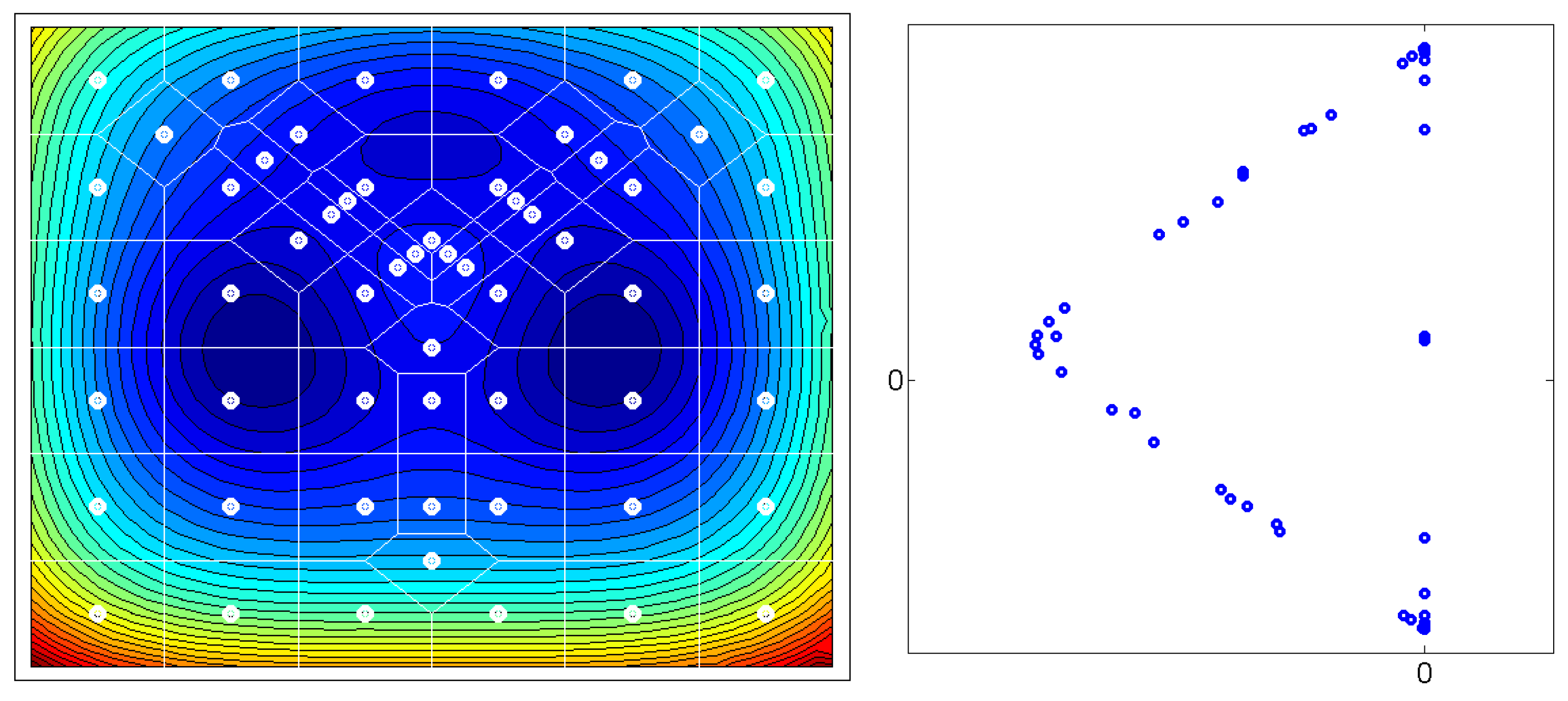According to the transfer operator theory and PCCA [3] the eigenvectors of these matrices were studied in the early 2000s leading to an empirical observation [4] and Figure 1: Given a matrix $X\in {\mathbb{R}}^{m\times n}$ of the $n\ll m$ leading eigenvectors of the $m\times m$-transition matrix P, the m rows of X – plotted as n-dimensional points – seem to always form an $(n-1)$-simplex. Some of those m points are located at the vertices of the simplices, other points are located on the edges. The points which are located at the n vertices of these simplices represent the thermodynamically stable conformations of the molecular systems. Whereas, the points which are located on the edges of the simplices represent transition regions. In order to transform the $(n-1)$-simplex ${\sigma }_1$ into the $(n-1)$-standard simplex ${\sigma }_0$ (spanned by the unit vectors), the inner simplex algorithm (ISA) [4] has been applied. ISA identifies those n points out of the m rows of X which are supposed to be the vertices of the simplex ${\sigma }_1$. These points are transformed into the unit vectors in ${\mathbb{R}}^n$ spanning ${\sigma }_0$. An easy introduction to ISA can be found online [5].

Mathematically, ISA transforms X via $\chi =X\mathcal{A}$ into an $m\times n$-matrix $\chi$. $\mathcal{A}\in {\mathbb{R}}^{n\times n}$ is a regular transformation matrix. The rows of $\chi$ are the new coordinates of the m points after transformation. If the simplex ${\sigma }_1$ was a perfect simplex, then the entries of the matrix $\chi$ are non-negative and the row sums of $\chi$ are one. This means, that the entries of $\chi$ can be interpreted as a partition-of-unity fuzzy clustering of the m subsets of $\Omega$ into n fuzzy sets. The membership values (denoted as membership functions) of these fuzzy sets are given by the columns of $\chi$. The theoretical justification for the distinction between thermodynamical stable regions and transition regions in $\Omega$, i.e., the described localization of the n-dimensional rows of X in an $(n-1)$-simplex, has been provided by Susanna Röblitz (chapter 3.1.2 in [6]).

Since the eigenvector data usually does not provide perfect simplices in real-world applications, ISA often results in a set of membership functions $\chi$ which have negative values [7].

The larger the deviation from the simplex structure, the higher are the absolute values of these negative entries. This can be employed to determine the number n of membership functions [7], such that the simplex structure is achieved. Besides this minChi-criterion, there exist other criteria for determining the number n. Of course, using a spectral gap in the sorted list of eigenvalues is one possibility. Another possibility is to construct a set-based clustering of states, such that the transition probabilities derived from the micro-process between these sets define a Markov chain [8]. One could also ask for a projection of the micro-process onto a Markov chain, such that the projection is as set-based as possible [6]. The next step is to compute the transformation matrix $\mathcal{A}$.

PCCA+ is an extension of ISA and was published in 2005 [9]. In some existing software codes the inner simplex algorithm (cluster_by_isa) is implemented and incorrectly denoted as PCCA+ like in [5]. PCCA+ assures that the transformation $\mathcal{A}$ is feasible in the following sense: the resulting membership functions are a partition-of-unity and the membership values are non-negative. Briefly, the linearly constrained feasible set $\mathcal{F}$ of transformation matrices is given by:

$$\chi =X\mathcal{A},\sum _{i=1}^n{\chi }_i\left(x\right)={11}_{\Omega },\chi \ge 0,$$

(1)

where ${11}_{\Omega }\equiv 1$ denotes a constant function.

The feasible set $\mathcal{F}$ is not empty and has an interior point (proof of Lemma 3.5 in [10]). Thus, the construction of a transformation matrix $\mathcal{A}$ is not unique. In PCCA+, the selection of $\mathcal{A}$ is given by solving a convex maximization problem. This means that there is a convex objective function $I\left[\mathcal{A}\right]$ to be maximized. The optimum of a convex maximization problem on a linearly bounded compact set is attained at a vertex of $\mathcal{F}$. PCCA+ is formulated as an unconstrained maximization problem $I\left[g\right(\mathcal{A}\left)\right]$, where the function g is a projection of an (infeasible) transformation matrix $\mathcal{A}$ onto a superset of the vertices of $\mathcal{F}$ (chapter 3 in [10]). The objective function $I\left[\mathcal{A}\right]$ accounts for the “crispness” of $\chi$. The membership functions should be as close as possible to characteristic functions of subsets of $\Omega$. One example for a possible objective function $I\left[\mathcal{A}\right]$ is provided at the end of Section 3.1. Solving the PCCA+ optimization problem can be very time consuming. Berg re-implemented PCCA+ with a fast Newton-type local optimization algorithm [11]. The implementation details of PCCA+ can be found in [12] and in Appendix D of [13]. In principle, the optimization problem to be solved has many local maxima. Local optimization routines cannot assure for finding the global optimum. However, there are possibilities to re-formulate PCCA+ as a linear optimization problem (chapter 3.4.3 in [10]) which has a unique global optimum. These possibilities have not been exploited in applications so far. Although PCCA+ is only one example for a spectral clustering routine, it is discussed that $\chi =X\mathcal{A}$, i.e., the mapping to a simplex, is spectral clustering [5]. It is also discussed in artificial intelligence that spectral clustering is (like PCCA+) a special way of a basis transform [14].

Taking some of the eigenvectors of a matrix P as the basis vectors of a linear subspace V is advantageous in terms of the matrix projection. Applying P to a vector $v\in V$ of this subspace produces a vector $w=Pv\in V$, which is again an element of V. Thus, V is said to be an invariant subspace with regard to P. All actions of P in the high-dimensional space can be projected onto actions of P within a low dimensional space V. This is denoted as “invariant subspace projection”.

Since its invention in 2005, a lot of scientific contributions extended the application area of PCCA+ and evolved the theory of PCCA+ into new directions. Until 2017, the original PCCA+ article has been cited more than 250 times PCCA+ is used as a spectral clustering method in various fields of application ranging from molecular simulation to psychology. Not only the areas of application changed, but also the theory of PCCA+ went into new directions:

• In contrast to PCCA+, GenPCCA is based on real invariant subspaces given by Schur decompositions [15]. This is useful, if the transition matrices have complex eigenvectors or are non-diagonalizable [16]. This extension of PCCA+ can be applied to non-reversible Markov chains.
• Treating non-autonomous processes is also possible, i.e., whenever transition probabilities of the Markov chain depend on external variables. In this case, these variables become additional coordinates of the state space of the Markov process. The analysis of metastable sets turns into a coherent sets analysis [17].
• PCCA+ has been invented for transition matrices. However, it can be applied to transfer operators or infinitesimal generators of time-continuous Markov processes as well [18]. In this case, adaptive discretizations of the operators play an important role [19,20].

Recently, the interpretation of $\chi =X\mathcal{A}$ as an equation which connects stochastics and numerics turned out to be a very fruitful link for computations in molecular sciences. The theoretical background of this equation will be explained in the next section.

Changing the point of view from a set-based towards a fuzzy clustering of $\Omega$ has some consequences: The set-based clustering allows for precise definition of transition states between macro-states at the interfaces of the sets [8]. In fuzzy clustering on the other hand, every micro-state in $\Omega$ is more or less a transition state. This type of fuzzy clustering is also known from the core set approach [21], where the degree of membership to one of the clusters is given by the probability to reach a certain subset of $\Omega$ by micro-dynamics before reaching certain other subsets. The PCCA+ approach is like a core set approach without the necessity to define core sets.

2. Interpretation of $\chi =X\mathcal{A}$

Many mathematical models in natural sciences are based on an input-output-relation. Given a certain (input) micro-state $x_0\in \Omega$ of a system, we want to predict its future (output) micro-states $x_t\in \Omega$, where t is the time-variable and $\Omega$ is some state space. These input-output-relations are often formulated as initial value problems of ordinary, stochastic, or partial differential equations, where these equations are first-order with regard to time-derivatives $\frac{\partial }{\partial t}$. Some examples are: Hamiltonian dynamics, Brownian motion, Langevin dynamics, Smoluchowski equation, Fokker-Planck equation, time-dependent Schrödinger equation, reaction kinetics, system biology models, etc. All these models can be seen as time-homogeneous (autonomous) Markov processes. All these processes are uniquely defined by their Markov kernel. The Markov kernel is a function

$$p:\Omega \times \Sigma \times [0,\infty ]\to [0,\infty ].$$

(2)

The first argument of p is a point $x\in \Omega$, which denotes the starting point of the micro-process. The second argument is a target subset $M\subset \Omega$, which has a measurable size. This is denoted by $M\in \Sigma$, where $\Sigma$ defines all measurable subsets of $\Omega$. The last argument is a time-span $\tau \in [0,\infty ]$. The function value $p(x,M,\tau )$ quantifies how likely a process starting in a micro-state $x\in \Omega$ will evolve into the (target) set $M\subset \Omega$ at time $\tau$. A good introduction into this theory can be found in Nielsen [22].

If we describe the properties of molecular processes, we often simplify the continuous state space $\Omega$ and speak of a finite set of macro-states. One example is the description of ligand-receptor-binding processes. Instead of providing all 3-dimensional coordinates $x\in \Omega$ of the ligand and of the receptor to describe the state of the system, we only discriminate between a finite number of macro-states, e.g., ‘bound’ vs. ‘unbound’. For every macro-state $i=1,\dots ,n$ there is a membership function

$${\chi }_i:\Omega \to [0,1],$$

(3)

which quantifies how much a micro-state $x\in \Omega$ belongs to i. Bujotzek established this approach for ligand-receptor binding processes [23,24,25].

On the one hand we have a Markov process (2), i.e., an input-output-relation on the level of micro-states. On the other hand, we only want to describe the process in terms of the macro-states (3). If a Markov kernel p is known for the micro-level it might be unknown for the macro-level. Even worse: On the macro-level the process need not be Markovian. A projected Markov process is in general not a Markov process anymore [26].

Example 1.

For example, take a particle that moves with regard to Brownian motion in a space Ω. This movement is a Markov process. Now we subdivide the space Ω into three subsets $A,B,$ and C. Thus, the particle has 3 macro-states $A,B$, and C. Once the particle crosses a barrier between two subsets, e.g., from A to B, it will more likely return to A than going to C, because of its jittering. In addition, if it crosses the barrier from C to B, it will more likely return to C than going to A. The conditional probability to move from B to one of the other sets is not independent from the past.

PCCA+ is a method for constructing the projection (3) in such a way, that the projected Markov process of micro-states is a Markov process again. The projected states are not only invariant subspaces, but they are also interpretable as macro-states (in terms of a fuzzy clustering of micro-states).

Here it is explained, how this projection works. Although the dynamics of the micro-system might be highly non-linear, it is possible to fully represent these processes by linear operators, namely by transfer operators. Transfer operators are given by solving an integral equation. In this context we will use Lebesgue integration. These integrals are based on measuring the size of subsets $M\in \Sigma$ with a so-called measure function $\mu \left(M\right)$. The set of all functions with finite Lebesque integral ${\int }_{\Omega }\left|f\left(x\right)\right|\mu \left(dx\right)$ is denoted as $L^1\left(\mu \right)$. Given a measure $\mu$, measurable sets $M\in \Sigma$, and a Markov kernel p, the transfer operator ${\mathcal{T}}^{\tau }:L^1\left(\mu \right)\to L^1\left(\mu \right)$ is defined by solving the integral equation

$${\int }_{\Omega }p(x,M,\tau )f\left(x\right)\mu \left(dx\right)={\int }_M\left({\mathcal{T}}^{\tau }f\right)\left(x\right)\mu \left(dx\right)$$

(4)

for all $M\in \Sigma$ and all $f\in L^1\left(\mu \right)$ chapter 1.2 in [22]. What is a transfer operator? In order to understand the meaning of transfer operators consider the following: If the Markov process is a Markov chain on a finite set of m states and $\mu$ is the stationary distribution of this chain, then the transfer operator is simply given by the transition matrix $P\in {\mathbb{R}}^{m\times m}$ of the Markov chain. ${\mathcal{T}}^{\tau }$ is a generalization of a transition matrix for continuous spaces $\Omega$.

Propagation of the micro-system is completely represented by the transfer operator ${\mathcal{T}}^{\tau }$, i.e., by a linear mapping. 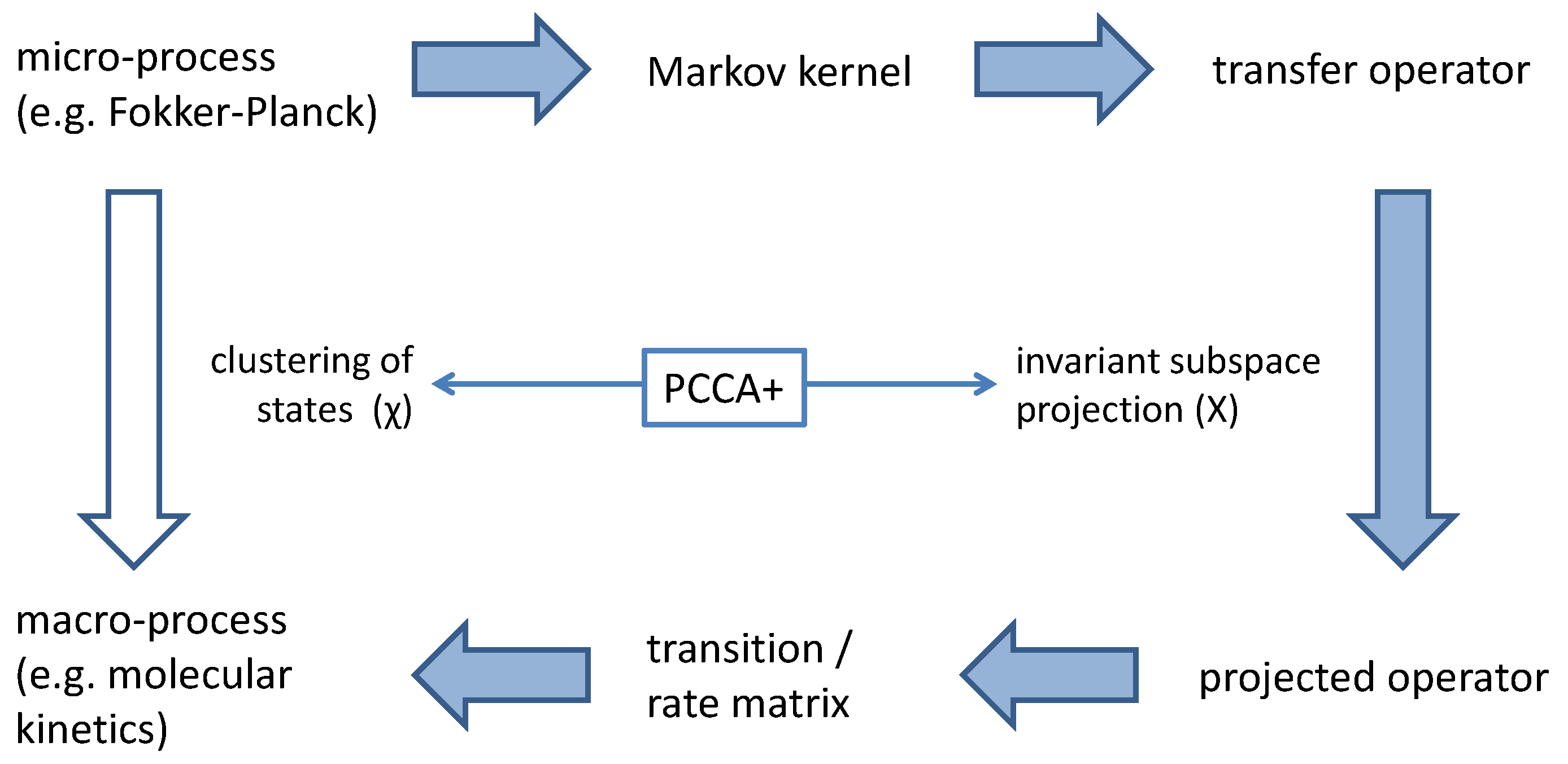If ${\mathcal{T}}^{\tau }$ has an n-dimensional invariant real subspace X, then propagation in the micro-system (starting with an element of that invariant subspace) can be projected onto a finite-dimensional linear mapping $T:{\mathbb{R}}^n\to {\mathbb{R}}^n$ within an n-dimensional vector space, i.e., onto an $n\times n$-matrix T representing the dynamics of the macro-system, consider Figure 2.

Invariant subspace projection of ${\mathcal{T}}^{\tau }$ is a suitable model reduction, but it is not the desired $\chi$-subset projection of $\Omega$. Equation $\chi =X\mathcal{A}$ provides now the recipe for constructing the functions $\chi$ such that the basis of the invariant subspace can be interpreted as membership functions of (fuzzy) subsets of $\Omega$. This is a three-step procedure:

• One has to find an n-dimensional invariant subspace X (real vector space) of the transfer operator of the micro-system. Real eigenspaces and real Schur spaces are suitable examples for invariant subspaces [6,15,18].
• Then one has to linearly transform the basis of this invariant subspace X in such a way, that all basis vectors form a non-negative partition of unity. This means, one has to search for a suitable transformation matrix $\mathcal{A}\in {\mathbb{R}}^{n\times n}$ which provides $\chi =X\mathcal{A}$.
• With the aid of $\chi$ it is possible to construct the projected transfer operator. This will be exemplified later in Equation (5).

This invariant subspace projection assures, that propagation with the linear transfer operator commutes with the projection from micro- to macro-systems [15,27]. The systematic error (described in [26]) of a set-based projection of ${\mathcal{T}}^{\tau }$ vanishes. The discussion of problematic recrossing events (see [28]) for the calculation of transition rates is not needed, if $\chi$ is computed via the described subspace projection.

3. Consequences of $\chi =X\mathcal{A}$

The invariant subspace projection of some transfer operator connects micro-systems to their macro-systems. The interpretation of $\chi =X\mathcal{A}$ as a state space clustering has interesting consequences for the modeling of molecular processes. In the followings, five consequences in different fields of molecular simulation and molecular modeling are sketched.

3.1. Rebinding Effects

Consider again the above example of a Brownian motion in Section 2, i.e., the particle that moves in between three subsets $A,B,$ and C of a (big) state space $\Omega$. Once the particle crosses a barrier between two sets, e.g., from A to B, it will probably recross that barrier $B\to A$. These recrossing events destroy the Markov property of the projected process [28]. In the field of molecular simulation, we know this recrossing event as well. Here it is known as rebinding [29]. Once a ligand molecule unbinds from its receptor, it is likely to observe a rebinding event because of the still close vicinity of ligand and receptor. A good mathematical review on this subject has been written by Röhl [30].

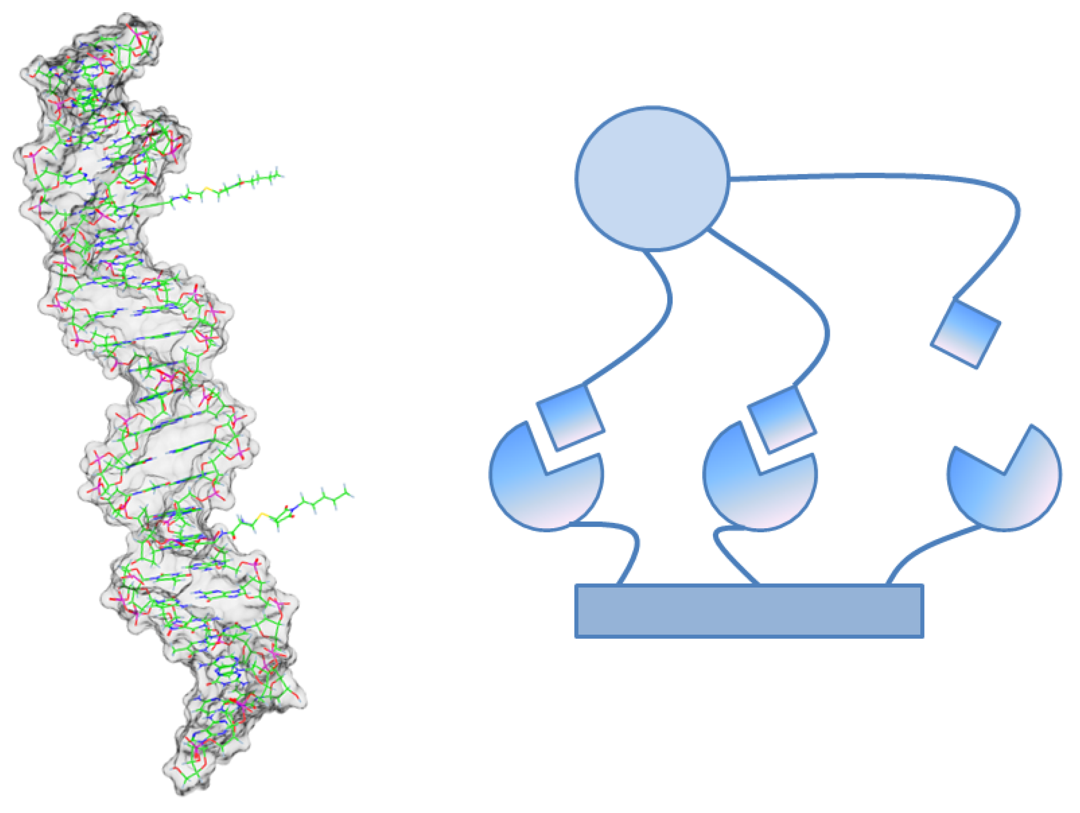
The rebinding phenomenon is especially relevant for multivalent ligand-receptor-binding [25,31]. In this case, the ligand has many “arms” that can individually bind to the receptor like in Figure 3. Although there is a highly frequent binding and unbinding of single arms, the total unbinding process of the multivalent ligand can be rather slow, because all arms have to unbind before one of the arms bind again. This complex multiscale binding process comprises of a lot of rebinding events and can be projected to a Markov chain on a small number n of macro-states by the methods explained above.

It has been shown that the representation of the projected Markov chain is given by a matrix $P=S^{-1}T\in {\mathbb{R}}^{n\times n}$. The projection theory of transfer operators has been worked out by Sarich [26]. The elements of the $n\times n$ stochastic matrices S and T are computed as follows

$$S_{ij}=\frac{{\langle {\chi }_i,{\chi }_j\rangle }_{\mu }}{{\langle {\chi }_i,{11}_{\Omega }\rangle }_{\mu }},T_{ij}=\frac{{\langle {\chi }_i,{\mathcal{T}}^{\tau }{\chi }_j\rangle }_{\mu }}{{\langle {\chi }_i,{11}_{\Omega }\rangle }_{\mu }},P=S^{-1}T,$$

(5)

where ${\langle ·,·\rangle }_{\mu }$ denotes the $\mu$-weighted scalar product and ${11}_{\Omega }(·)\equiv 1$ is a constant function. $\chi =X\mathcal{A}$ are the membership functions of the macro-states. There is a relation between these matrices and the transformation matrix $\mathcal{A}$. If ${\mathcal{T}}^{\tau }$ is self-adjoint (reversible Markov process) and $\mu$ is the stationary density of the micro-process, then $S=D^{-1}{\mathcal{A}}^T\mathcal{A}$, $T=D^{-1}{\mathcal{A}}^T\Lambda \mathcal{A}$, and $P={\mathcal{A}}^{-1}\Lambda \mathcal{A}$, where $\Lambda$ is the diagonal matrix of the n leading eigenvalues of ${\mathcal{T}}^{\tau }$ and $D=\mathrm{diag}({\langle {\chi }_i,{11}_{\Omega }\rangle }_{\mu })$ the diagonal matrix of the stationary distribution of the macro-process [32].

In the reversible case, a matrix exists – $Q={\tau }^{-1}{\mathcal{A}}^{-1}\ln (\Lambda )\mathcal{A}$ – where $\ln (\Lambda )$ is the diagonal matrix of the logarithm of the eigenvalues. This matrix generates P, i.e, $P=\exp \left(\tau Q\right)$, where $\exp (·)$ denotes the matrix-exponential.

Let us assume that P is generated by a rate matrix Q. Rate matrices have non-negative off-diagonal elements, these are the rates between the macro-states (chapter 4 in [34]). The diagonal elements of Q are negative real numbers, such that the row sums of Q are zero. Thus, the sum of all rates of the system is given by the negative trace of the matrix Q (Equation (3.1) in [32]):

$$\begin{array}{ccc}\hfill -\mathrm{trace}\left(Q\right)& =& -{\tau }^{-1}\ln \left(\exp \left(\mathrm{trace}\left(\tau Q\right)\right)\right)\hfill \\ & =& -{\tau }^{-1}\ln \left(\det \left(\exp \left(\tau Q\right)\right)\right)\hfill \\ & =& -{\tau }^{-1}\ln \left(\det \left(P\right)\right)\hfill \\ & =& {\tau }^{-1}\left(\ln \left(\det \right(S\left)\right)-\ln \left(\det \right(T\left)\right)\right).\hfill \end{array}$$

Due to the fact that S and T are stochastic matrices, their determinants cannot be larger than 1. The case $\det \left(S\right)=\det \left(T\right)=1$ only occurs, if T and S are unit matrices. If there are frequent transitions on the micro-level of the process (binding events of the “arms”), the stochastic matrix T will have a low-valued determinant (Theorem 4.4 in [10]), i.e., the negative logarithm will be a high number. Thus, the sum of the rates of the macro-processes tends to be high. However, the overlap of the membership functions, represented by the matrix S can compensate for that: If the membership functions have a significant overlap, then also the determinant of S is small which leads to a decreased sum of rates. The determinant of S, therefore, is used as a measure of the stabilization of a process on the macro-level due to rebinding effects. For reversible micro-processes the matrix $S=D^{-1}{\mathcal{A}}^T\mathcal{A}$ directly depends on the transformation matrix $\mathcal{A}$, if we take into account that the diagonal elements of D are given by the first row of $\mathcal{A}$ (Lemma 3.6 in [10]). It turns out, that the minimal rebinding effect that is included in a measured (binding) kinetics can be quantified and estimated [30]. According to a suggestion of Röblitz, PCCA+ searches for a transformation matrix $\mathcal{A}$ such that the trace of the matrix S is maximized [6], which will also lead to high values of $\det \left(S\right)$. This means, that PCCA+ tries to minimize the rebinding effect (i.e, tries to minimize re-crossings).

3.2. Exit Rates

Equation $\chi =X\mathcal{A}$ can be used to compute important dynamical properties from molecular simulations. A full decomposition of the state space $\Omega$ into macro-states is often not mandatory. For exit rate computations it is only needed to know how long it would take until a molecular process starting in a point $x=x_0\in M$ (of some subset $M\subset \Omega$) leaves this subset. In particular it is asked for the exit rate, the holding probability, and the mean holding time of the set M. The connection between these values and operator theory is very well explained by Pavliotis in [35]. As an example, $M\subset \Omega$ could define the ‘bound’ macro-state of a ligand-receptor-system. The holding probability is defined by the following expectation value:

$$p_{11_M}(x,t)=\mathbb{E}{\left[{11}_M\left(x_t\right)·{\delta }_0\left({\int }_0^t(1-{11}_M\left(x_r\right))dr\right)\right]}_{x_0=x}.$$

(6)

$11_M:\Omega \to \{0,1\}$ is the characteristic function of the set M. ${\delta }_0:\mathbb{R}\to \{0,1\}$ is a discontinuous function with ${\delta }_0\left(0\right)=1$ and ${\delta }_0(·)=0$ elsewhere. The expectation value is computed over an ensemble of trajectories $x_r\in \Omega ,$ with $r\in [0,t],$ for realizations of a suitable stochastic process starting in $x_0=x$. Only trajectories which start in M and never leave M in the interval $[0,t]$ are counted in (6).

We want to extend this approach towards continuous membership functions $\chi :\Omega \to [0,1]$ instead of sets. In PCCA+, these membership functions $\chi$ are computed from an invariant subspace of some transfer operator ${\mathcal{T}}^{\tau }$. Here, we assume that the transfer operator is generated by an infinitesimal generator $\mathcal{L}$ with ${\mathcal{T}}^{\tau }=\exp \left(\tau \mathcal{L}\right)$. In this case, $\chi$ can equivalently be computed from a real invariant subspace of $\mathcal{L}$, i.e., for a 2-macro-state example there exist via PCCA+ real numbers ${ϵ}_1,{ϵ}_2\in \mathbb{R}$, such that

$$\mathcal{L}\chi =-{ϵ}_1\chi +{ϵ}_2({11}_{\Omega }-\chi ).$$

(7)

By multiplying this equation with the expression $e^{-{ϵ}_{1}t}$, and by defining a function $p_{\chi }(x,t):=\chi \left(x\right)e^{-{ϵ}_{1}t}$, we equivalently get:

$$\mathcal{L}{p}_{\chi }-{ϵ}_2\frac{1-\chi }{\chi }{p}_{\chi }=-{ϵ}_1{p}_{\chi },$$

(8)

for all $x\in \Omega$ with $\chi \left(x\right)\ne 0$. The definition of $p_{\chi }$ can be expressed by an ordinary differential equation:

$$\frac{\partial p_{\chi }}{\partial t}=-{ϵ}_1{p}_{\chi }\mathrm{and}{p}_{\chi }(x,0)=\chi \left(x\right).$$

(9)

Combining Equations (8) and (9) leads to the following differential equation:

$$\frac{\partial p_{\chi }}{\partial t}=\mathcal{L}{p}_{\chi }-{ϵ}_2\frac{1-\chi }{\chi }{p}_{\chi },p_{\chi }(x,0)=\chi \left(x\right).$$

(10)

More details can be found online [36]. For a special choice of the infinitesimal generator $\mathcal{L}$, Equation (10) is the solution of the following conditional expectation value problem according to the Feynman-Kac formula (Equations III.1 and III.2 in [37]):

$$p_{\chi }(x,t)=\mathbb{E}{\left[\chi \left(x_t\right)·\exp \left(-{ϵ}_2{\int }_0^t\frac{1-\chi \left(x_r\right)}{\chi \left(x_r\right)}dr\right)\right]}_{x_0=x}.$$

(11)

In this expression, $x_t\in \Omega$ are realizations of molecular processes starting in $x_0=x$ and generated by $\mathcal{L}$ (more precisely, by the adjoint of $\mathcal{L}$).

Equation (11) is like the relaxed version of Equation (6) replacing sets by membership functions. This means, that given a membership function $\chi$ with the PCCA+ property of Equation (7), the holding probability of the corresponding fuzzy set is given by Equation (11) which decreases exponentially with $p_{\chi }(x,t)=\chi \left(x\right)e^{-{ϵ}_{1}t}$ and with exit rate ${ϵ}_1$. Given the eigenfunction f of ${\mathcal{T}}^{\tau }$ with ${\mathcal{T}}^{\tau }f=\lambda f$ and the PCCA+ construction $\chi ={\alpha }_{1}f+{\alpha }_2{11}_{\Omega }$, then ${ϵ}_1$ can be computed by ${ϵ}_1=-{\tau }^{-1}\ln \left(\lambda \right)+{\alpha }_2$. The mean holding time for the membership function $\chi$ and for a starting point $x\in \Omega$ is therefore:

$$t_{\chi }\left(x\right)={\int }_0^{\infty }{p}_{\chi }(x,t)dt=\chi \left(x\right)\frac{1}{{ϵ}_1}=\frac{\chi \left(x\right)}{-{\tau }^{-1}\ln \left(\lambda \right)+{\alpha }_2}.$$

(12)

In this way, Equation $\chi =X\mathcal{A}$ can be used for finding simple analytical relations between fuzzy sets in state space $\Omega$ and special dynamical properties of the molecular systems. In the above case, the computations of exit rates ${ϵ}_1=-{\tau }^{-1}\ln \left(\lambda \right)+{\alpha }_2$, holding probabilities $p_{\chi }(x,t)=\chi \left(x\right)e^{-{ϵ}_{1}t}$, and mean holding times $t_{\chi }\left(x\right)$ are directly connected to the PCCA+ construction of $\chi$.

3.3. Kinetic ITC

Isothermal titration calorimetry (ITC) is an experimental approach to measure thermodynamical quantities of chemical processes [38]. Ligand-receptor binding processes are often analyzed with this tool. One possible experimental setup can look like this: To an isolated reaction tube with a certain resolved concentration of receptors a certain amount of ligands is added successively in each step of the ITC measurement (titration). By adding the ligand, the temperature of the reaction tube changes. Assuming an endothermic reaction (i.e, the temperature tends to decrease), we have to warm up the reaction tube in order to keep its temperature constant [39]. If the ligand-receptor-binding is a fast process, then heat must be added quickly. For a slow ligand-receptor-binding, the external heating is also slow to always assure constant temperature. This means, that the electric power used for heating is a monitor for the rate of the binding process. The binding rate can be calculated from the power profile. This calculation is named kinetic ITC (kinITC) [40].

The kinITC experiment provides the rate of a process which starts with a certain concentration of receptors, ligands, and (at consecutive titration steps) already formed ligand-receptor-complexes. It ends with a thermodynamically equilibrated mixture of those components in each titration step. The micro-processes taking place in the reaction tube are, thus, projected to these two macro-states, ‘unbound’ and ‘bound’. The macro-process is assumed to be Markovian: Only the initial concentrations of the components have to be known in order to explain the experimental outcome. Thus, according to Section 2 and Section 3.1 we assume the existence of a $2\times 2$-matrix P which is the invariant subspace projection of the Markovian micro-process.

The experimental setup of kinITC does not allow for a direct calculation of the matrix P. Instead of P, kinITC provides its infinitesimal generator $Q\in {\mathbb{R}}^{2\times 2}$ with $P=\exp \left(\tau Q\right)$ and $\tau$ being the time-interval of each titration step. Q is assumed to be a rate matrix which depends on the initial concentration of the unbound ligand $c_{lig}$ to be measured directly after titration:

$$Q=\left(\begin{array}{cc}-k_{12}{c}_{lig}& k_{12}{c}_{lig}\\ k_{21}& -k_{21}\end{array}\right).$$

(13)

Using the measured ITC experimental data, the binding rate $k_{12}$ and the dissociation rate $k_{21}$ can be estimated for each step of the titration [41]. Usually, these rates are assumed to be constants. In real experiments, they systematically vary in each titration step.

These variations can be explained by the formula $\chi =X\mathcal{A}$. In some cases Q can be calculated theoretically by the subspace projection. If we can model the micro-processes taking place in the reaction tube, e.g., by knowing the multi-step reaction kinetics network of the binding process, we can directly access the infinitesimal generator $\mathcal{L}$ of ${\mathcal{T}}^{\tau }$ in each step of the titration. Let us assume, e.g., a two step reaction. After binding of the ligand (micro-state 1 to micro-state 2), the ligand-receptor-complex undergoes a conformational change (micro-state 2 to micro-state 3). In this case:

$$\mathcal{L}=\left(\begin{array}{ccc}-r_{12}{c}_{lig}& r_{12}{c}_{lig}& 0\\ r_{21}& -(r_{21}+r_{23})& r_{23}\\ 0& r_{32}& -r_{32}\end{array}\right),$$

(14)

with suitable reaction rates $r_{12},r_{21},r_{23},r_{32}$ which do not depend on $c_{lig}$.

We can (analogously to Equation (5)) compute the invariant subspace projection of $\mathcal{L}$ onto Q by applying PCCA+ to the respective eigenvectors of the “operator” $\mathcal{L}$. In each step of the titration, the infinitesimal generator $\mathcal{L}$ (i.e., its eigenvectors) depend on the initial concentration of the unbound ligands. 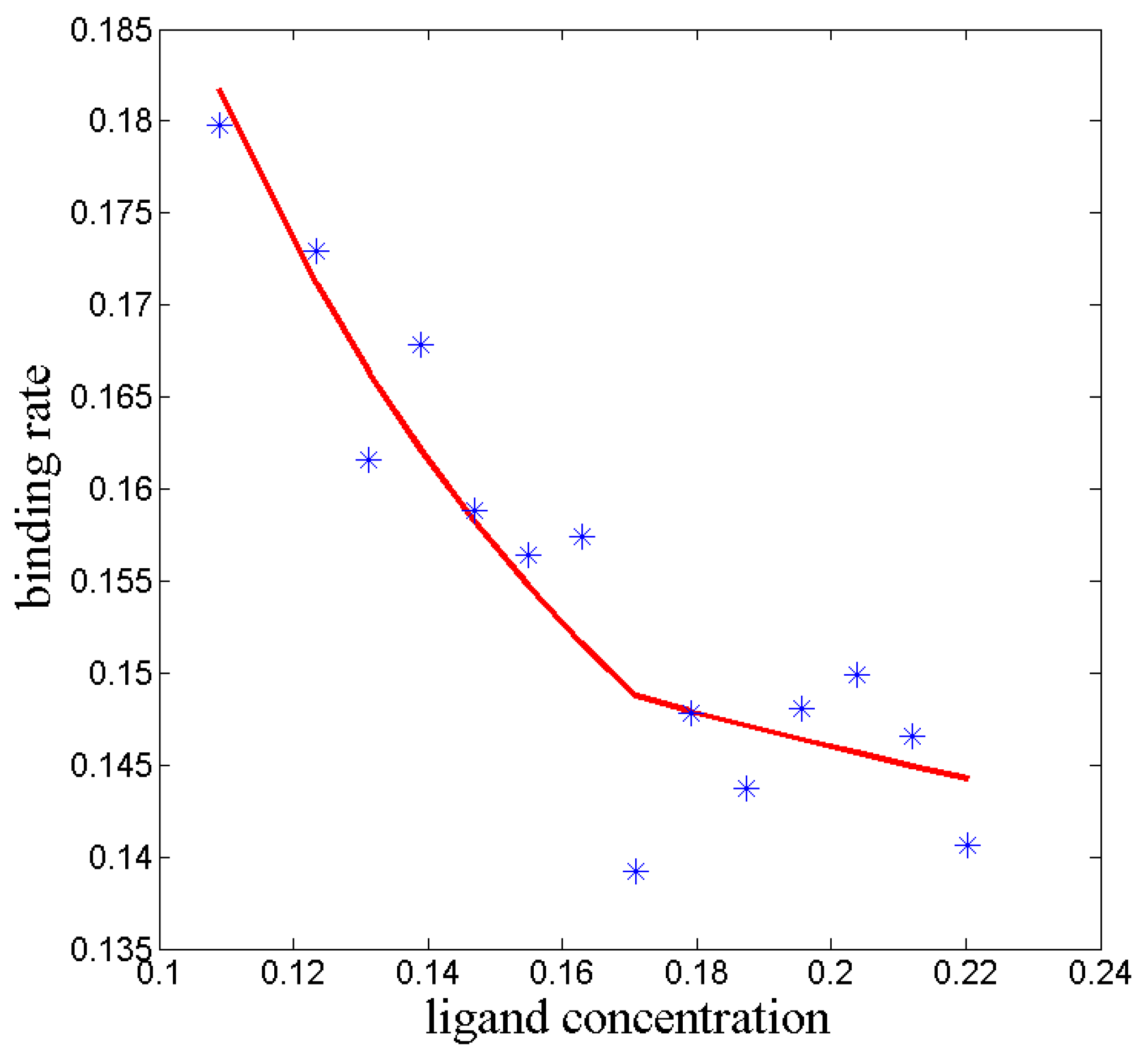Hence, the projection Q, i.e., the rates $k_{12}$ and $k_{21}$, depend on $c_{lig}$ as well. A parameter fitting of the multi-step reaction network can, thus, explain the systematic changes of the rates in Q during the kinITC experiment, see Figure 4.

3.4. Pericyclic Reactions

PCCA+ is usually applied to eigendecompositions of finite transition matrices of reversible Markov chains. Discrete approximations $P\in {\mathbb{R}}^{m\times m}$ of transfer operators ${\mathcal{T}}^{\tau }$ are estimated by generating a sample of molecular dynamics trajectories of length $\tau$ and counting transitions between (pre-defined) subsets M of $\Omega$. From a mathematical point of view, the Markov kernel $p(·,·,\tau )$ in Equation (2) is, thus, computed for only a few initial points $x\in \Omega$ and a few disjoint sets $M\in \mathcal{B}(\Omega )$. Equation (4) is only solved for those functions f which are the characteristic functions of the given subsets. In molecular simulation, these approximations of ${\mathcal{T}}^{\tau }$ are denoted as Markov State Models generated by an analysis of short- or fragmented long-term molecular trajectories. A very good introduction into Markov State Modeling can be found in [42]. Another method to construct transfer operators is called Dynamic Mode Decomposition which will be subject of Section 3.5 below.

In Section 3.3 it has already been indicated that the estimation of the infinitesimal generator $\mathcal{L}$ can be an alternative approach to receive the desired invariant subspace information X without computing ${\mathcal{T}}^{\tau }=\exp \left(\tau \mathcal{L}\right)$ explicitly. The square root approximation (SQRT-A) is a computational method for estimating a discrete version of $\mathcal{L}$, i.e., a rate matrix $L\in {\mathbb{R}}^{m\times m}$ which represents a suitable approximation of the dynamics of the micro-system [43,44]. The matrix L is used to approximate the invariant subspace of ${\mathcal{T}}^{\tau }$ and to find the desired set of $n\ll m$ membership functions for projection of the micro-process onto an n-states macro-process.

Consider a decomposition of $\Omega$ into m disjoint subsets and $\mu \in {\mathbb{R}}^m$ to be the stationary distribution of the Markov process restricted to these m subsets. SQRT-A defines the transition rate between neighboring subsets i and j as $L_{ij}=\sqrt{{\mu }_j/{\mu }_i}$ . All other off-diagonal elements of L are zero, because only between neighboring subsets instantaneous transitions are possible. The diagonal elements of L are constructed such that the row sums of L are zero, i.e., L becomes a non-dissipative rate matrix.

SQRT-A can easily be extended towards the case of a time-dependent density $\mu \left(t\right)$ with $t\in [0,\Theta ]$. In this case the matrix L is generated in the already described way, but instead of only decomposing $\Omega$ into m subsets the larger space $\Gamma :=\Omega \times [0,\Theta ]$ is decomposed and the neighborhood relation is extended to consecutive time steps as well.

This procedure is especially very useful, if solely the time-dependent evolution of a density function $\mu \left(t\right):\Omega \to \mathbb{R}$ of states in $\Omega$ at time t is known. In other words: Whenever the individual trajectory of each “particle” of that moving density is unknown we can only exploit the information about $\mu \left(t\right)$. One example is given by an electron density $\mu \left(t\right)$ that is propagated via the time-dependent Schrödinger equation in the 3-dimensional space $\Omega ={\mathbb{R}}^3$, where the “movement” of every single electron is not known [45].

Whereas the SQRT-A matrix L stemming from a time-independent density $\mu$ represents a reversible Markov process by construction, in the time-dependent $\mu \left(t\right)$-case the SQRT-A is usually non-reversible. Eigenvalues and eigenvectors may be complex-valued. Real invariant subspaces have to be constructed via Schur decomposition, i.e., for Schur values close to the value 0 (see also [17]). After constructing an invariant subspace X and after applying $\chi =X\mathcal{A}$, the membership functions are approximately spanning the kernel space of L, i.e., $L\chi \approx 0$. This means, that the “particles” which generate the time-dependent density will rarely cross the boundaries of the fuzzy sets ${\chi }_1,\dots ,{\chi }_n$. This information can be used to reconstruct electron movement during pericyclic reactions (see chapter 4.3.7 in [45] and Figure 5 and Figure 6).

3.5. Sequential Spectroscopy

In the field of spectroscopy, several spectra (d-dimensional non-negative vectors) are often measured sequentially in given time intervals. In most cases, closed molecular systems are observed, e.g., by sequential Raman spectroscopy. Each individual measured spectrum (also called “signal”) is the average of many ensemble signals of the components of the mixture. If we assume that each molecule (or atom, or electron) of the mixture can be assigned to a small number of n macro-states, which can interconvert into each other by micro-processes, then the measured signal is always a convex combination of n corresponding high-dimensional vectors $v_1,\dots ,v_n\in {\mathbb{R}}^d$. Depending on the ratio (concentration) of components of the mixture in each of the n states, the weights of this convex combination are changing over time [46]. The time-dependent measured signal is:

$$v\left(t\right)=\sum _{i=1}^n{\chi }_i\left(t\right)v_i,$$

(15)

where ${\chi }_i\left(t\right)$ is the convex combination factor of the signal $v_i$ corresponding to state i at time t. “Convex combination” means that all these factors are non-negative and that the sum ${\sum }_{i=1}^n{\chi }_i\left(t\right)=1$ is the unity. If we assume that the measurements are carried out at m equally spaced points in time $t_1,\dots ,t_m\in [0,\infty )$ with $t_{i+1}=t_i+\tau$ for a constant interval $\tau$, then the convex combination factors can be arranged in a matrix $\chi \in {\mathbb{R}}^{m\times n}$, which is a row stochastic matrix, i.e., it obeys Equation (1). The measurements can be arranged in a matrix $V\in {\mathbb{R}}^{m\times d}$. This matrix V is usually non-negative due to the physics of spectroscopy. The n “pure” d-dimensional spectra $v_1,\dots ,v_n$ can be arranged in an $n\times d$ non-negative matrix W.

The mathematical problem to be solved in sequential spectroscopy is to find the dimension n and the matrices $\chi$ and W given the matrix V, such that $V=\chi W$ is a non-negative matrix factorization of V, whereas $\chi$ is a row-stochastic matrix.

PCCA+ can be used to solve this problem [47]. Note that all convex combinations of n vectors in a d-dimensional space with $d\gg n$ are included in an $(n-1)$-dimensional affine linear subspace of ${\mathbb{R}}^d$. Following steps lead to the solution:

• In order to transform the affine linear space into a linear subspace, one could for example subtract the mean vector $\overline{v}$ (taking the mean over all measurements) from all rows of V. This leads to a normalized matrix $\overline{V}=V-{11}_m{\overline{v}}^T$, where ${11}_m$ is an m-dimensional constant vector, all elements are 1.
• If the assumptions for solving the problem are correct, then $\overline{V}$ should have rank $n-1$. Together with a singular value decomposition $\overline{V}=\overline{X}\Sigma \overline{Y}$, this can be used to determine n.
• We know that the columns of the matrix $\chi$ span a linear space in which the vector ${11}_m$ is included. Thus, after determining n and $\overline{X}$, we construct the n-dimensional linear space $\{{11}_m,{\overline{x}}_1,\dots ,{\overline{x}}_{n-1}\}$ by accounting for the first $n-1$ column vectors ${\overline{x}}_i$ in $\overline{X}$. With the aid of Gram-Schmidt orthogonalization, this basis of a linear space can be transformed into an orthogonal basis with ${11}_m$ being the first basis vector. The n orthogonalized basis vectors are organized in a matrix $X\in {\mathbb{R}}^{m\times n}$. This matrix provides the linear space for the convex combination factors, i.e., there must be a linear transformation $\mathcal{A}\in {\mathbb{R}}^{n\times n}$, such that $\chi =X\mathcal{A}$.
• Given the matrix X constructed from the spectral data, PCCA+ applied to X will provide a row-stochastic matrix $\chi$ which is the proposed matrix of concentrations. Thus, PCCA+ solves the problem.

However, due to errors in measurement and maybe due to deviations from the affine linear space, the matrix $W={\chi }^{\#}V$ constructed from the pseudo-inverse of $\chi$ need not be non-negative. Röhm [47] analyzed in his master’s thesis, whether it is useful to include an additional term (which measures the deviation of W from a non-negative matrix) into the objective function $I\left[\mathcal{A}\right]$ of PCCA+. It turned out, that this does not improve the results of $\chi$ significantly.

Dynamic Mode Decomposition [48] can help to improve the PCCA+ result, i.e., to provide a better transformation matrix $\mathcal{A}$ from a physical point of view. If the measured dynamical process takes place in a closed environment, then it is assumed to be autonomous. In this case, there should be an unknown stochastic transition matrix $P\in {\mathbb{R}}^{n\times n}$, i.e., according to Section 2 there should be a projected transfer operator for the $\tau$-discretized process. If ${\chi }_{i,•}$ is the i-th row of $\chi$, then ${\chi }_{i+1,•}={\chi }_{i,•}P$ provides the concentration vector for the next step. Thus, we construct ${\chi }_{-}$ which includes the first $m-1$ rows of $\chi$ and we construct ${\chi }_{+}$ which includes the last $m-1$ rows. For these matrices we get ${\chi }_{+}={\chi }_{-}P$. By using $\chi =X\mathcal{A}$, we get $\overline{P}:=\mathcal{A}P{\mathcal{A}}^{-1}=X_{-}^{\#}{X}_{+}$, where $X_{-}$ and $X_{+}$ are constructed from X analogously. Thus, $\overline{P}$ can directly be constructed from the measured data. 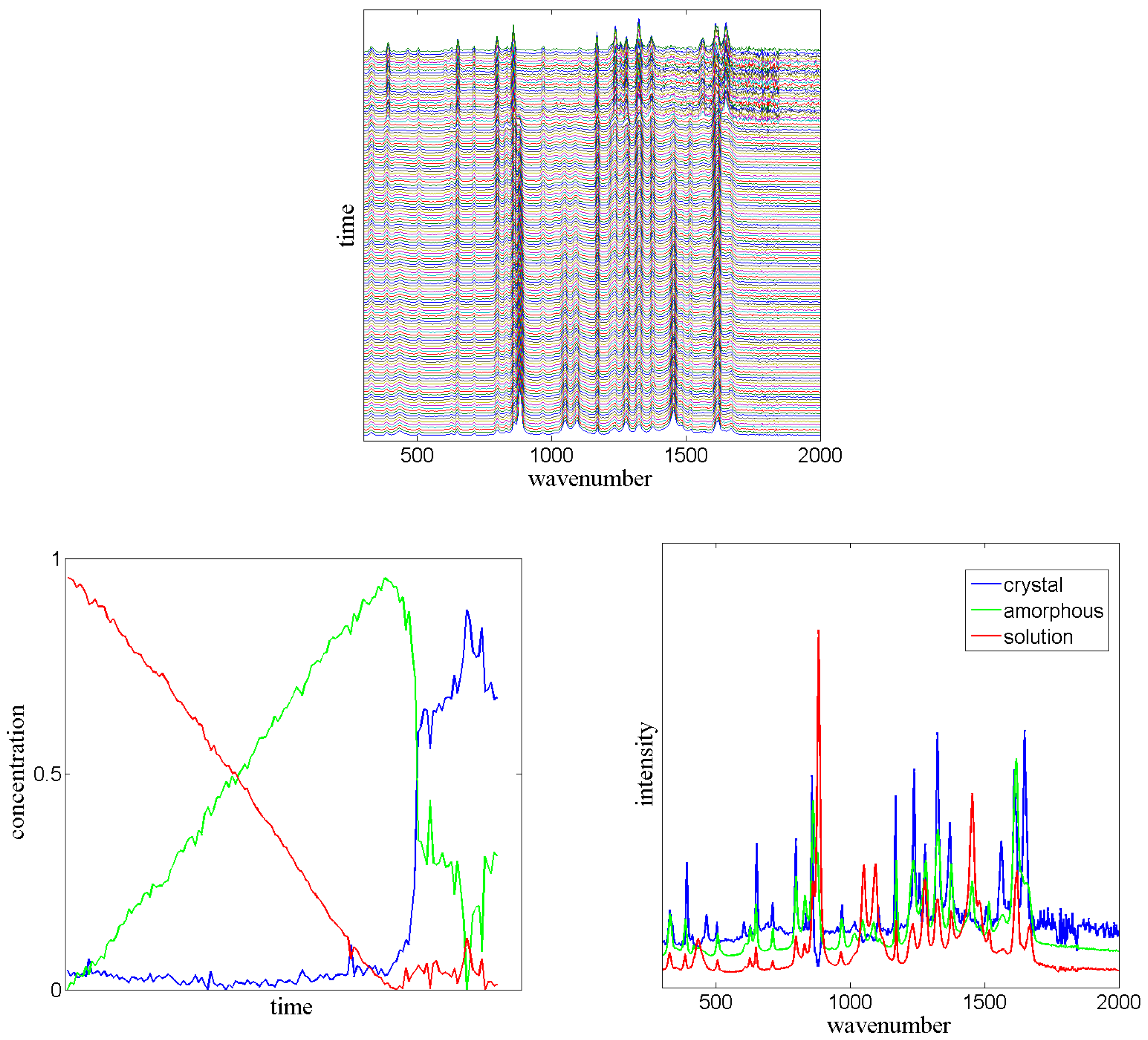In PCCA+, $\mathcal{A}$ must be searched in such a way that ${\mathcal{A}}^{-1}\overline{P}\mathcal{A}$ is a stochastic matrix. This additional criterion improves the solution of the sequential spectroscopy problem, see Figure 7.

4. Conclusions

PCCA+ is not only a clustering algorithm for reversible Markov chains. Given a Markov process on a micro-level, PCCA+ is the recipe for projecting this process onto a Markov macro-process.

The main Equation $\chi =X\mathcal{A}$ of PCCA+ provides the corresponding invariant subspace projection. It explains, how macro-states have to be defined. The definition is based on invariant subspaces of the linear transfer operator of the micro-process. This kind of defining macro-states has conceptual consequences in different fields of molecular simulation or molecular sciences.

Whenever implications for the macro-process should be derived from micro-processes, Equation $\chi =X\mathcal{A}$ plays an important role. PCCA+ is a way to determine the “unknown” $\mathcal{A}$ of this equation. $\mathcal{A}$ is the solution of an optimization problem, which tries to project the micro-process onto a few Markov macro-states such that recrossings between the macro-states are rare events.