Article

Multiresolution Modeling of Semidilute Polymer Solutions: Coarse-Graining Using Wavelet-Accelerated Monte Carlo

by
Animesh Agarwal
1,*,
Brooks D. Rabideau
2 and
Ahmed E. Ismail
3,*
1
Institute for Mathematics, Freie Universität Berlin, Berlin 14195, Germany
2
Department of Chemical and Biomolecular Engineering, University of South Alabama, Mobile, AL 36688, USA
3
Department of Chemical and Biomedical Engineering, West Virginia University, Morgantown, WV 26506, USA
*
Authors to whom correspondence should be addressed.
Computation 2017, 5(4), 44; https://doi.org/10.3390/computation5040044
Submission received: 21 August 2017 / Revised: 20 September 2017 / Accepted: 25 September 2017 / Published: 28 September 2017
(This article belongs to the Special Issue Computation in Molecular Modeling)

Abstract

:
We present a hierarchical coarse-graining framework for modeling semidilute polymer solutions, based on the wavelet-accelerated Monte Carlo (WAMC) method. This framework forms a hierarchy of resolutions to model polymers at length scales that cannot be reached via atomistic or even standard coarse-grained simulations. Previously, it was applied to simulations examining the structure of individual polymer chains in solution using up to four levels of coarse-graining (Ismail et al., J. Chem. Phys., 2005, 122, 234901 and Ismail et al., J. Chem. Phys., 2005, 122, 234902), recovering the correct scaling behavior in the coarse-grained representation. In the present work, we extend this method to the study of polymer solutions, deriving the bonded and non-bonded potentials between coarse-grained superatoms from the single chain statistics. A universal scaling function is obtained, which does not require recalculation of the potentials as the scale of the system is changed. To model semi-dilute polymer solutions, we assume the intermolecular potential between the coarse-grained beads to be equal to the non-bonded potential, which is a reasonable approximation in the case of semidilute systems. Thus, a minimal input of microscopic data is required for simulating the systems at the mesoscopic scale. We show that coarse-grained polymer solutions can reproduce results obtained from the more detailed atomistic system without a significant loss of accuracy.

1. Introduction

Despite rapid advances in computational power in recent decades, realistic simulation of polymers remains a major scientific challenge because of the enormous range of time and length scales that must be accessed. To address this challenge, numerous solution paradigms have been introduced. One approach has been through so-called multiresolution simulation, in which a single computational routine that is capable of consistently simulating a system at different length scales is developed. In this manner, different simulations can be studied at a common length scale by appropriately coarse-graining a given model without switching between the different simulation methods. These methods are different from common coarse-graining techniques, which are adequate for studying the large-scale features of a system, but usually address the system at just two different levels of detail [1,2,3,4,5,6,7,8,9].
Recently, several approaches have been proposed that use a single computational routine to model the system using a hierarchy of different resolutions. Pandiyan and co-workers [10] devised a hierarchical multiscale scheme where high temperature polyimide HFPE-30 was coarse-grained at three different levels of detail, and the structural properties were reproduced at each of the resolutions. Lyubarstev et al. [11] formulated a hierarchical multiscale approach that covered three different levels of description by using inverse Monte Carlo (IMC). Yang et al. [12,13] developed structure- and relative-entropy-based coarse-graining methods for homopolymer melts and compared the structural and thermodynamic properties of the original and the coarse-grained (CG) systems at various coarse-graining levels. Zhang et al. [14] developed an elegant hierarchical coarse-graining and reverse-mapping strategy to model high molecular weight polymer melts, mapping the atomistic chains onto a model of soft spheres with fluctuating size.
The wavelet-accelerated Monte Carlo (WAMC) method developed by Ismail et al. [15,16,17,18,19] is a multiresolution approach capable of forming a sequence of resolutions of a system within one computational scheme, allowing for feasible computation without distorting the large-scale structural features of the system. As the wavelet transform is recursive, it produces averaged objects, which can be further averaged to provide a much coarser representation of a given system; therefore, the explicit construction of mapping from atomistic to CG representation is not required [19]. Thus, it is a systematic strategy that can model a system with an arbitrary number of length scales and may be particularly useful for systems that are so large that modeling with only two levels of coarse-graining remains insufficient. The WAMC technique was successfully applied to freely jointed and self-avoiding chains using up to four stages of coarse-graining. It was shown that the method preserves sensitive measures from the fine-grained calculations such as the mean end-to-end distance and the radius of gyration. Furthermore, as a result of the reduction in the number of degrees of freedom, independent configurations could be generated with a speedup of up to seven orders of magnitude.
A similar approach was used by Chen et al. [20] to simulate DNA molecules by fitting the CG potentials to analytical functions for additional computational efficiency. Maiolo et al. [21] formulated the wavelet-based MSCG approach and demonstrated its robustness through studies modeling liquid water and methanol. In addition to the aforementioned sequential multiscale methods, concurrent multiscale simulation approaches have also been developed in the last decade, where the coupling between the atomistic and CG regions allows for “on-the-fly” particle exchange [22,23].
Our goal in this paper is to extend the work on topological coarse-graining of polymer chains to a fully-functional and hierarchical approach for coarse-graining polymers solvated by good solvents in the semidilute regime. This is done by determining the potentials between coarse-grained units using simulations at one length scale and deriving new potentials at different resolutions through the use of scaling laws. This allows one to tune the WAMC algorithm so that the potentials are not recalculated when changing the resolution, something that would not be possible for algorithms operating at fixed levels of coarse-grained resolution. Thus, using the results of single chain statistics (zero-density simulations), we develop potentials that are transferable to finite densities in the semi-dilute regime. The major advantage of such an approach is that a minimal input of microscopic data or fine-grained simulation is required to simulate polymer chains at different coarse-grained resolutions.
The remainder of the paper is organized as follows: In the first section, we give an overview of the wavelet transform and WAMC algorithm. In the second section, we derive bonded and non-bonded (intramolecular) potentials and parameterize the potentials for different levels of coarse-graining for off-canticle polymer systems. In the third section, we formulate the modified WAMC algorithm for multiple polymer chains and make an approximation to compute the intermolecular potential. In the last section, we report the technical details of the simulations and compare the results obtained with the WAMC algorithm to reference off-lattice simulations. The Results and Discussion section is divided into two parts. The first deals with the simulation of single polymer chains (zero-density limit), while the second part deals with multiple polymer chains (finite density). In the zero-density limit case, we have considered two different scenarios: polymer chains both in an athermal solvent, where the interaction beads are defined by a hard sphere potential, and in a good solvent, where the interaction beads are defined by a Lennard–Jones potential.

2. Methods

2.1. The WAMC Method

2.1.1. Wavelet Transform Representation of a Polymer Chain

A one-dimensional wavelet transform is comprised of two functions: a scaling function α and a wavelet function β . A mathematical object is decomposed into two components that represent averages and differences, using the functions α and β . Suppose there is a “signal” u = [ u ( 1 ) , u ( 2 ) , u ( 3 ) , , u ( n ) ] . If the functions α and β are applied to this signal, then one obtains a set of averages s ( i ) and a set of differences δ ( i ) [24,25]:
s ( i ) = k = 0 r 1 α ( k ) u ( i + k ) , δ ( i ) = k = 0 r 1 β ( k ) u ( i + k ) ,
where r defines a length scale where α and β are nonzero functions with compact support in the range [ 0 , r 1 ] . The coefficients of α and β are usually in the range [ 1 , 1 ] , and both α and β can assume negative values [24]. In the previous work [15,16], the Haar wavelet was used, with r = 2 , α = [ α ( 0 ) , α ( 1 ) ] = ( 1 / 2 , 1 / 2 ) and β = [ β ( 0 ) , β ( 1 ) ] = ( 1 / 2 , 1 / 2 ) [26]. The application of the wavelet transform is straightforward for polymer chains, as they are inherently topological in structure [2,27]. The coarse-grained representations can be easily created using the connectivity of the polymer chains as a template. If the input data are the set of positions of the beads within the polymer chain, R = { r 1 , r 2 , , r N } , then the following variables are obtained:
r n ( k ) = 1 2 [ r 2 n 1 ( k 1 ) + r 2 n ( k 1 ) ] , w n ( k ) = 1 2 [ r 2 n 1 ( k 1 ) r 2 n ( k 1 ) ] .
r n ( k ) denotes a set of averages { r i ( k ) } i = 1 N / 2 ( k ) , and w n ( k ) denotes a set of differences { w i ( k ) } i = 1 N / 2 k , where the superscript notation ( k ) denotes the number of times that the Haar wavelet transform has been applied. The averaging operator in Equation (2) creates a new coarse-grained bead r n ( k ) at the center of mass of the beads at r 2 n 1 ( k ) and r 2 n ( k ) , and the differencing operator returns the distance between the position of one of the original particles and the center of mass. Figure 1 shows the coarse-graining of a self-avoiding random walk in two dimensions, as described by the wavelet transform method. After two iterations, four sites are created that lie on quarter-integer lattice points. We neglect the contributions of the differencing variables in the remainder of this work.

2.1.2. Wavelet-Accelerated Monte Carlo Algorithm

The main idea behind the wavelet-accelerated Monte Carlo (WAMC) algorithm is the division of the full-atomistic simulation into different stages, where each stage is treated separately at coarse-grained resolution [15,16]. The algorithm is detailed as follows:
  • The WAMC algorithm starts with a full-atomistic simulation of a smaller segment of the initial chain with N b , 1 N beads. A simulation of a much shorter segment of the fully-atomistic chain helps cut down on the computational cost. Thus, each bead still has an effective size N e , 1 = 1 , where the subscript ”1” indicates the simulation stage.
  • The subsystem is sampled using the pivot algorithm [28].
  • The wavelet transform is applied K 1 times to obtain the positions r ( K 1 ) of each coarse-grained bead at regular intervals of O ( N b , 1 ) steps. The effective size of the coarse-grained bead corresponds to N e , 2 = 2 K 1 beads in the fully-atomistic representation. The distribution representing interactions between these “virtual” coarse-grained beads, which are also referred to as “superatoms”, is calculated.
  • The probability distributions obtained from the the first stage are then used in the second stage of the (real) simulation that consists of a chain of length N b , 2 beads ( N b , 2 = N / N e , 2 ). The effective size of the coarse-grained bead is N e , 2 , and the total effective chain length is N b , 2 × N e , 2 .
  • If desired, further coarse-graining of the system occurs by transferring the probability distributions obtained from the current stage to the next stage of resolution as discussed above.
Figure 2 is the schematic representation of the original WAMC method.

2.1.3. Translate-Jiggle Algorithm

The translate-jiggle algorithm [29] is used to generate trial conformations of the coarse-grained chain since the length of an individual bond does not change if the pivot algorithm is used, which makes the pivot algorithm non-ergodic for sampling chains where the bond-length is variable. Thus, a different algorithm is required to simulate a coarse-grained polymer chain, which requires correct sampling of the probability distributions obtained from the original level. In the translate-jiggle algorithm, a bead is selected randomly (k) and is given a random displacement. As a consequence, the bond between between beads k and bead k 1 will be either stretched or compressed, which ensures that the previous bond lengths between remain constant. After defining the displacement vector for bead k, all the remaining beads ( k + 1 , k + 2 ,..., N) undergo the same vector transformation. The resulting chain is then tested for energy differences using the Metropolis Monte Carlo algorithm [30] to determine if the proposed configuration is either accepted or rejected. Since the internal coordinate distributions were already calculated in the preceding stage of the WAMC algorithm, a new bond length and orientation ( r i , ϕ i , θ i ) are selected from these distributions to be used in the translate-jiggle algorithm. This ensures that the coarse-grained model reproduces the aforementioned distributions given sufficient sampling.

2.2. Potentials in a Coarse-Grained System

The complete set of CG interaction functions can be separated into bonded and non-bonded interactions, which are each obtained separately. The potential energy of a coarse-grained chain can be written as:
U CG = U CG B + U CG N B ,
where the superscripts B and N B refer to the bonded and non-bonded interactions, respectively [31]. First, we discuss the non-bonded potentials, with a discussion of the bonded interactions following later.

2.2.1. Non-Bonded Potentials

There are various methods available in the literature for constructing non-bonded (intramolecular) potentials between CG beads. One notable approach is to consider the polymer coils as soft particles and to replace the detailed interactions between the segments with an effective interaction acting between the center-of-mass of polymer coils [32,33]. This effective interaction is equivalent to the potential of mean force obtained by Boltzmann inversion of the center of mass distribution of the polymer chains. The resulting potential is finite at all distances and has a range on the order of the radius of gyration. In this work, we use a method similar to the method developed by Dautenhahn and Hall [34]. This method was designed to calculate the potential to a high degree of accuracy, which is desirable in our work as we want to correlate the potential for different polymer sizes. In the next sections, we report the technical aspects of this method, and how we obtain a universal potential function from the functions calculated for different values of N e .

Construction of Coarse-Grained Force Fields

A self-avoiding polymer chain of length N e monomers, where N e is the number of monomers coarse-grained in the original chain of length N b × N e , is simulated using the pivot algorithm and used to generate two sets of 500 conformations of the polymer chain. In this work, the hard-sphere radius is taken as σ = 0 . 5 . Therefore, two monomers are considered to overlap if they are separated by a distance less than r c u t = 2 σ = 1 . Independent conformations are generated each time the number of accepted pivot algorithm moves is equal to the chain length [35]. In this way, 1000 independent conformations are generated, and two sets of single-chain conformations, each containing 500 conformations for N e = 32 , 64 and 128, are used in calculating U ( r ) . One conformation from each set is placed with its center of mass a given distance at a random orientation. The distance between the centers of mass of two chains is varied from 0–5-times the average radius of gyration R g of the chain with spacing equal to 0.2 R g . The following relation is used to calculate the statistical weight of each configuration at a given separation:
W i ( r ) = exp ϕ i ( r ) k B T ,
where W i ( r ) is the weighting of the two-chain configuration i, r is the distance between the centers of mass of the two chains and ϕ i ( r ) is the potential between the two chains in configuration i. The potential of mean force between the chains, U ( r ) , is calculated as a function of the distance between the two centers of mass using the following relation [34]:
U ( r ) k B T = ln i = 1 M W i ( r ) M
where M is the total number of two-chain configurations used at that particular distance. For self-avoiding chains with no overlap between the conformations, the potential is ϕ i ( r ) = 0 , and the statistical weight of the configuration is W i ( r ) = 1 . If the two chains overlap, then ϕ i ( r ) = and W i ( r ) = 0 .
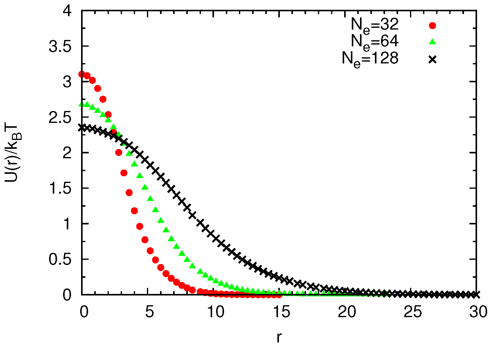
Figure 3 shows the potential obtained for three different polymer chains of length N e = 32 , 64 and 128. As expected, the potential is short-ranged and finite even at small separations. There is no attractive potential between the chains. There is a weak repulsion at very small distances indicating that some of the conformations are able to interpenetrate without monomer overlap when the centers of mass of the two chains coincide. As the chain length increases, there is an increase in the number of such conformations since the chains can arrange themselves in an increasing number of different ways. According to Equation (5), the repulsive potential decreases as the number of such configurations increases. As we are only working with a two-chain system or an infinitely-diluted system, the potential of mean force calculated above represents the true potential between the polymer “soft particles”, since entropy has a negligible contribution to the free energy of the interaction. At finite densities however, the many-body interactions produce a nonzero entropic contribution, and this relation no longer holds.

Universal Scaling

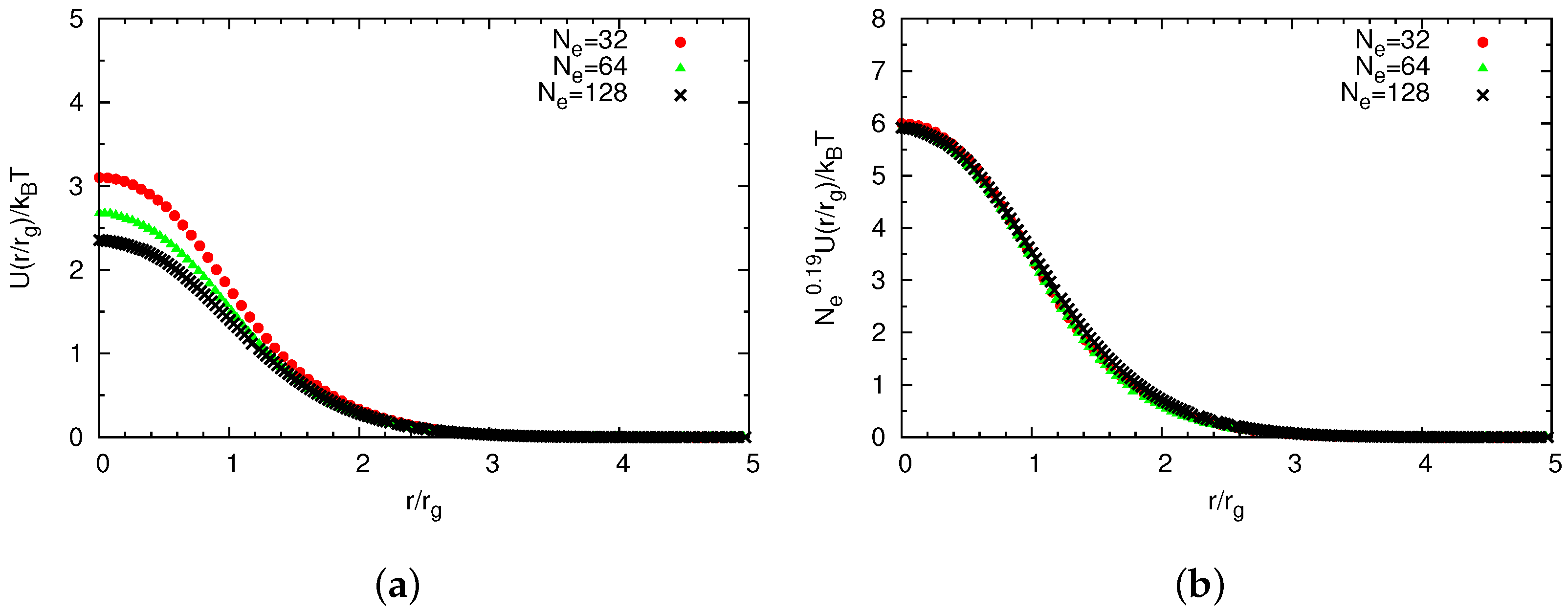
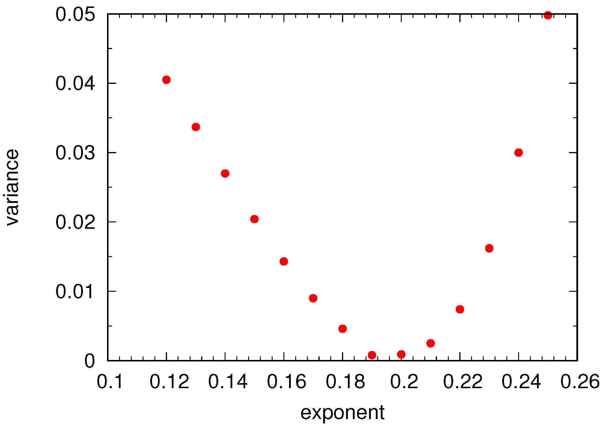
The motivation for using wavelet-accelerated Monte Carlo (WAMC) is to analyze the polymer system on different length scales, without the need for recomputing the potentials as the scale is changed. Hence, it is important to have a universal function that gives the potential function at any length scale using scaling laws. Since the radius of gyration is a measure of the size of the polymer chain and is often used to scale results for the different chains, we normalize the distance by the root mean square radius of gyration of the coarse-grained bead of size N e . Figure 4a shows the potentials for athermal chains of length N e = 32 , 64 and 128 with the normalized distance. It can be seen that the potential functions for different chain sizes are considerably different for r / r g < 2 . Figure 4b shows that the different potentials can be collapsed onto a single function by scaling the energy by N e 0 . 19 . Consequently, we do not need to recalculate the potential. The exponent 0 . 19 was determined by using trial and error. A plot of the variance in the values of U ( 0 ) for the three chains after scaling is shown in Figure 5.

2.2.2. Bonded Potentials

While non-bonded potentials act between pairs of CG beads separated by three or more intervening beads, we assume that nearest, next-nearest and next-next-nearest neighbor pairs are governed by separate interaction potentials:
U bonded = U i , i + 1 + U i , i + 2 + U i , i + 3 ,
where the three terms indicate nearest neighbor (or 1–2), next-nearest neighbor (1–3) and next-next-nearest neighbor (1–4) interactions, respectively. These interactions are computed in such a way that the distributions of the 1–2, 1–3 and 1–4 distances are identical in the atomistic and coarse-grained cases. If the distributions computed from the atomistic simulation are P atom ( r i ) and the distributions from the coarse-grained system are P CG ( r i ) , then the potentials should be such that P atom ( r i ) = P CG ( r i ) . We note that bond, angle and torsion potentials are not used to calculate the energy of chains. However, as discussed earlier, during the “translate-jiggle” moves, when a bead is randomly displaced, the values of ( r , θ , ϕ ) can be taken from the distributions of the bond length, bond angle and torsion angle calculated from the atomistic simulations. This ensures that lower energy states are adequately sampled with respect to angle and dihedral energy functions. The total potential energy of a single polymer chain can be written as:
U intra = i = 1 N 1 ϕ i , i + 1 bonded ( r i j ) + i = 1 N 2 ϕ i , i + 2 bonded ( r i j ) + i = 1 N 3 ϕ i , i + 3 bonded ( r i j ) + i = 1 N 4 j = i + 4 N ϕ i , j non bonded ( r i j )
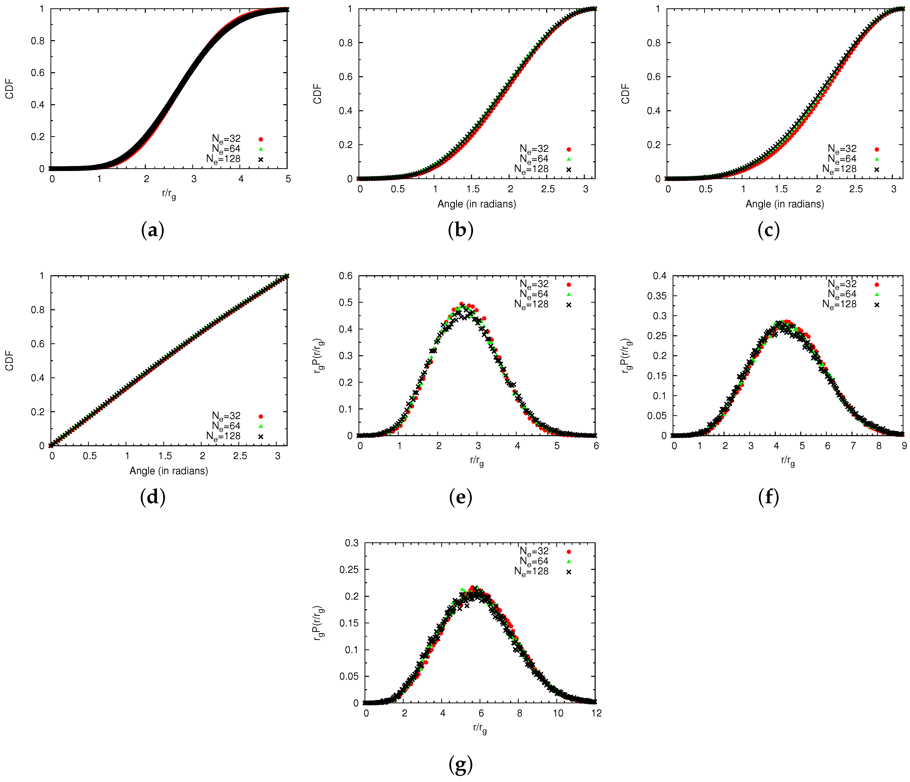
The neighbor distributions, as well as the cumulative bond length, angle and dihedral angle distributions, which are used in the translate-jiggle moves, are calculated using a self-avoiding polymer chain of length N = 1024 for different values of N e . The potentials are determined through the use of an iterative procedure known as reverse Monte Carlo [6,36], which can compute the interactions when there are interdependent distributions and the entropic contributions cannot be neglected in the free energy of the interaction. In the following sections, we give an overview of the method and find the common functions for the potentials obtained for different values of N e . Figure 6 shows the various distributions that have been obtained for use in the reverse Monte Carlo routine.

Reverse Monte Carlo Simulations

A reverse Monte Carlo simulation of a coarse-grained system updates the potential according to:
ϕ new ( r ) = ϕ old ( r ) + f k B T ln P ( r ) measured P ( r ) target
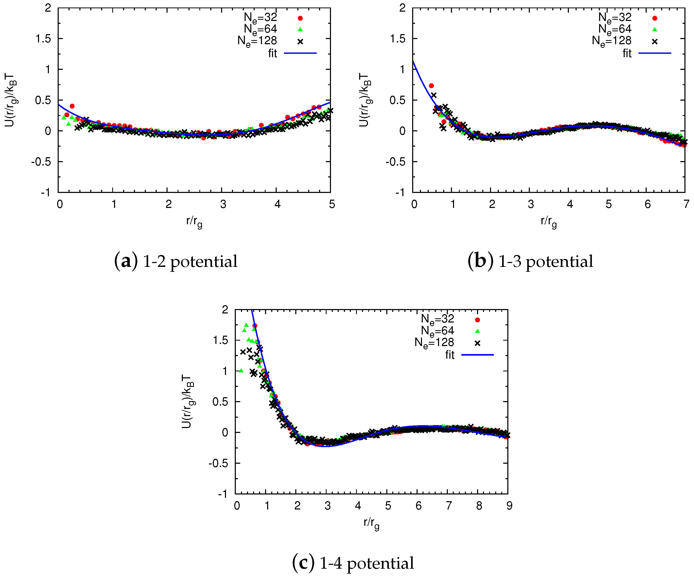
where f = 0 . 2 is chosen to ensure stable convergence. In this method, an initial guess of the potential is first used, and the simulation yields a probability distribution function P ( r ) measured , which may be different from the target distribution function P ( r ) target , but can also be used to obtain a first correction to the potential. This process can be iterated until the distribution function and the potential are self-consistent. This method has been used to calculate the 1–2, 1–3 and 1–4 interactions, with target distributions calculated from the atomistic system. In this work, the initial guess for the potential is taken to be ϕ ( r ) = 0 . This proved to be a reasonable assumption as the measured distributions converged to the target distributions in just a few iterations. The potentials obtained after this procedure are shown in Figure 7 for N e = 32 , 64 and 128. In the next section, we find common functions for the potentials obtained by polynomial fitting, to avoid further RMC calculations when changing the scale of coarse-graining.

Universal Scaling

To obtain the universal functions, we parameterize these potentials by normalizing the distance with the radius of gyration of the CG bead. Thus, the bonded and non-bonded potentials both have common functions, which can be tuned for different sizes of the coarse-grained bead. This ensures that the potentials need not be recalculated as the scale of the system is changed. We fit the 1–2 potential to a quadratic polynomial and the 1–3 and 1–4 potentials to a sixth-degree polynomial (see Figure 7). If the probability of finding the neighbors at a certain distance is zero, then the potential at that distance is not calculated. Hence, the softness of these potentials as r 0 remains unclear due to the absence of data at these distances. It can be seen in Figure 7c that below r / R g < 0 . 5 , the potential goes to infinity, which corresponds to zero probability of finding the next-nearest neighbors in Figure 6g. This assumption works well, giving accurate results and retaining the distributions in the coarse-grained model. The 1–2 potential shows a very small attractive well ( 0 . 1 k B T ) at r / R g 0 . 5 . Overall, the potential varies from 0 . 1 k B T to 0 . 4 k B T , which is quite small. However, as mentioned earlier, during the translate-jiggle moves, we used the values of r, θ and ϕ from the distributions calculated from the atomistic simulation. This ensures that the bond length distributions are sampled effectively, leading to a lower bond energy. The 1–3 and 1–4 potentials show an oscillatory behavior, with a strong repulsive core followed by a small attractive well. The 1–3 potential ranges from 0 . 2 k B T at r / R g = 1 to 0 . 1 k B T around r / R g = 1 . 7 , while the 1–4 potential varies from k B T at r / R g = 1 to 0 . 7 k B T around r / R g = 2 . 7 . The 1–2 and 1–3 neighbors pay a significantly lower energy penalty compared to 1–4 neighbors for r / R g 1 . Since the 1–4 potential has a much higher energy penalty for r / R g 1 , it makes it highly unlikely that the 1–4 pairs approach each other. The range of the repulsive core in the 1–4 potential is comparable to that of the non-bonded potential.

3. Extension to Semidilute Systems

In the semidilute regime, additional interactions must be added to the coarse-grained representation when compared with the single-chain model, which have to be evaluated separately. To compute these interactions, a few approximations are introduced. Our aim is to develop these potentials from the knowledge of single-chain statistics so as to enable transferability of the force field to different densities.

3.1. Semidilute Solutions

The coarse-grained representation of many-chain systems consists of intramolecular interactions between coarse-grained beads in a single chain and intermolecular interactions between beads in different chains:
U t o t a l = U i n t r a + U i n t e r ,
where
U i n t r a = i = 1 M U i n t r a ,
and
U i n t e r = i = 1 M 1 a = 1 N b j = i + 1 M b = 1 N b U i n t e r ,
where U i n t e r is the pairwise potential between two beads on different chains, M is the total number of chains in the system and N b is number of coarse-grained beads in each chain. The intermolecular potential acts between all the beads of one particular chain and all the beads in the other chains.
There are different ways to construct the intermolecular potential. The most obvious way is to simulate the fully-atomistic system and construct an inter-segment distance distribution function, which can then be used to obtain the potential through Boltzmann inversion. This is a particularly useful approach for simulating the system on one length scale, although it becomes cumbersome if the scales of the system are continuously changed, as is done in this work.
As mentioned earlier, our goal is a potential that can be easily transferred to different densities and resolutions. In light of this requirement, we assume that the intermolecular potential is equal to the non-bonded potential calculated in the previous section, so that U i n t e r = ϕ n b . This assumption holds for dilute systems, where many-body interactions can be neglected, and the potential of mean force represents the actual potential. Furthermore, as shown by Pierleoni et al. [37,38], this assumption works well even for semidilute systems. If the number N b of coarse-grained beads per chain is such that the coarse-grained bead density is below the overlap density of the coarse-grained beads, then it is expected that zero-density potentials between different chains can be safely used (see the Appendix for a justification of the conditions under which the zero-density potentials can be used). Under such assumptions, the total energy can be written as:
U t o t a l = i = 1 M U i n t r a + i = 1 M 1 a = 1 N b j = i + 1 M b = 1 N b ϕ n b .
With the distributions from the single chain, we can simulate a coarse-grained semidilute polymer system. We expect the force field to work for all polymer volume fractions satisfying Equation (A3) under athermal conditions. The force field has to be recalculated for different temperatures; however, at different densities and levels of coarse-graining at a given temperature, it should yield the correct results.

3.2. Modified WAMC Algorithm for Semidilute Solutions

The WAMC algorithm has been previously employed to model a single freely-jointed chain [15,16]. In this work, we have modified the algorithm to simulate semi-dilute solutions of polymer chains. The algorithm is outlined as follows:
  • We define a dilute/semi-dilute polymer system containing M polymer chains, where each polymer chain consists of N beads.
  • The first stage is an atomistic simulation in the limit of zero density to calculate intermolecular and intramolecular potentials discussed in the previous sections. The number of atomistic beads represented by a coarse-grained bead is N e = 1 in the first stage, by definition.
  • Next, the finite density polymer system is coarse-grained by iterating Equation (2) K 1 times, so that the size of each coarse-grained bead is N e = 2 K 1 in the second stage. We then calculate the true potentials from the universal functions shown in Figure 4 and Figure 7.
  • If the level of coarse-graining is sufficient, then we can stop after this coarse-grained simulation. Otherwise, we apply the wavelet transform (Equation (2)) again K 2 times to obtain coarse-grained beads with an effective size of N e = 2 K 2 .
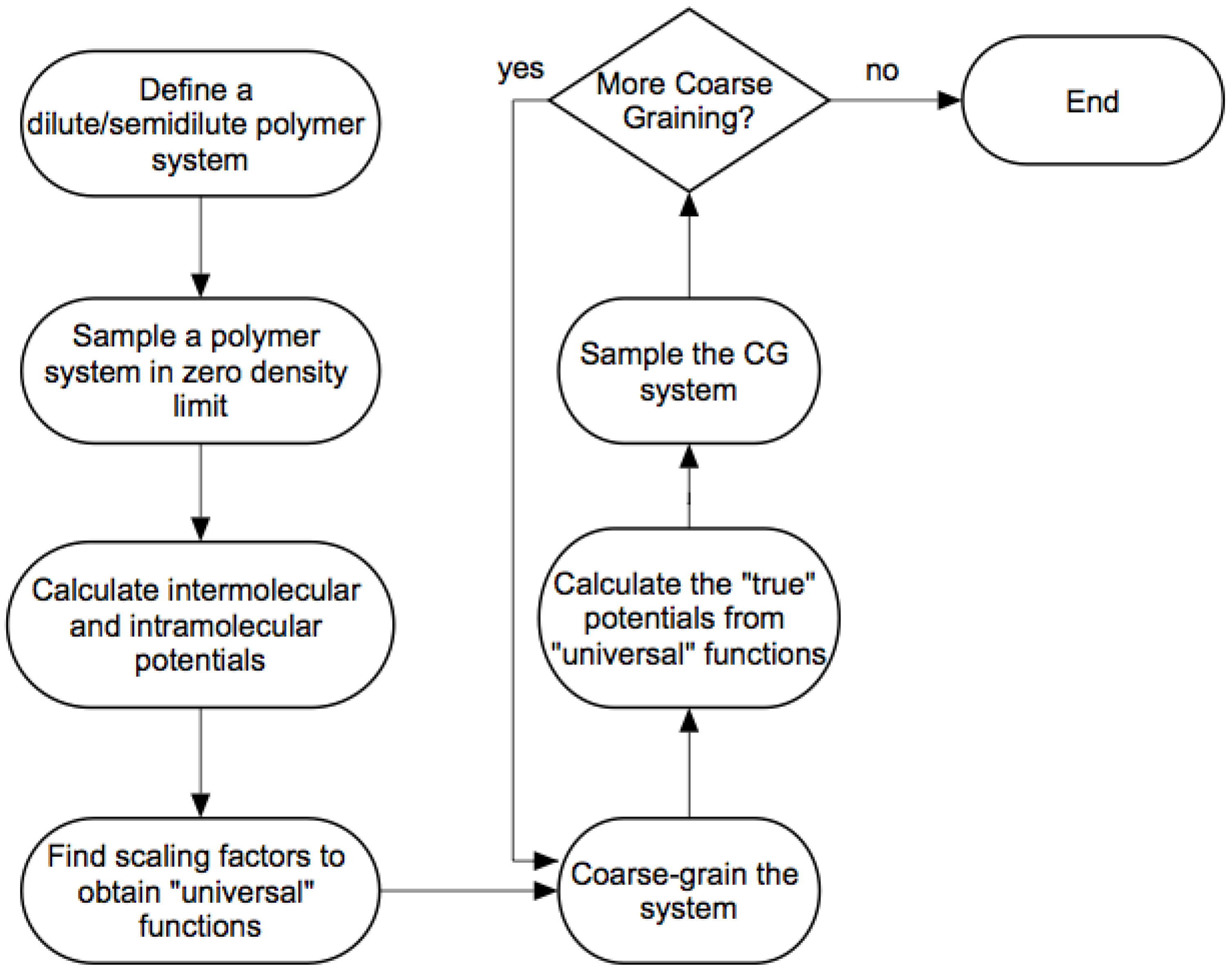
Figure 8 shows a flowchart describing the various steps of the modified algorithm.

4. Results and Discussion

4.1. Single Chains

4.1.1. Technical Details

We perform simulations of off-lattice polymer chains of varying lengths using the atomistic freely-jointed model and the coarse-grained model under two levels of coarse-graining N e = 32 and 64. The trial conformations of the freely-jointed chain model are generated using the pivot algorithm, and the Metropolis criterion is subsequently used to accept or reject the trial conformation. In an athermal solvent, a trial conformation is rejected if any two monomers appear closer than one distance unit. We test the WAMC model for polymer chains in good solvents. Although our simulations do not explicitly include solvent molecules, their interaction with the polymer chains is effectively accounted for by considering a Lennard–Jones type of potential between the monomers that has a small attractive well.
By changing the well depth ϵ / k B T , the interaction of the solvent with the polymer chains is taken into account. Thus, ϵ / k B T can be viewed as the polymer-polymer potential modified by polymer-solvent and polymer-polymer interactions. We assume that there is no energetic interaction between covalently connected beads, while all other neighbors interact with a truncated LJ potential:
U ( r i j ) = 4 ϵ σ r i j 12 σ r i j 6 for r i j r o = 0 for r i j > r o
where r i j is the distance between two monomers, ϵ and σ are the energy and distance parameters associated with the potential model and r o is the distance at which the potential is truncated.
The parameters in this study are taken from a study of polyethylene [39], in which a single sphere constituted 3.5 methylene units where ϵ = 400 and σ = 4 . 6 Å. The cutoff radius r o was taken to be 2.5 σ . Furthermore, the important physical quantity in our simulation is the well depth ϵ / k B T , which defines the attractive part of the LJ potential. The greater | ϵ / k B T | is, the greater the attraction. We simulate the polymer chains for three values of | ϵ / k B T | : 0.0 (athermal system), 0.10 and 0.15. This represents the good solvent regime, which was determined by calculating the theta point, which lies around ϵ / k B T 0 . 25 . We simulate freely-jointed chains of length N = 2 5 = 32 to N = 2 13 = 8192 for ϵ / k B T = 0 . 0 , 0 . 10 , 0 . 15 and determine the scaling factor for each system: ν = 0 . 604 , 0.599 and 0.590 for ϵ / k B T = 0 . 0 , 0 . 10 and 0 . 15 , respectively.
Using these scaling relations, we determine the size of the chains of length N = 2 14 and 2 15 . The second set of simulations is performed on the coarse-grained model of a freely-jointed chain at three different values of ϵ / k B T under two levels of coarse-graining: N e = 32 and 64, where N e represents the size of the CG bead or number of monomers coarse-grained. The total number of beads in the coarse-grained model was N b = N / N e . For the coarse-grained simulations, the “translate-jiggle”algorithm described in Section 2.1.3 was used. The potential functions for different N e were extracted from the fitted functions for the force field derived.

4.1.2. Comparison of Coarse-Grained and Atomistic Results

We compare the atomistic model and the coarse-grained model by calculating the mean squared radius of gyration and the Flory exponent ν in the polymer scaling law, R N ν . The calculation of the radius of gyration provides a good platform to compare the original “atomistic” and coarse-grained models, as the size of the polymer coil should be similar in the two models. Table 1 shows the mean-squared radius of gyration obtained from the atomistic and coarse-grained models under different solvent conditions, as a function of ϵ / k B T . It can be seen from these results that the values obtained from the coarse-grained models agree quite well with the results from the atomistic simulation. The values obtained from the CG simulation lie within 3% of the values obtained from the freely-jointed chain simulations.
As ϵ / k B T decreases, the mean-squared radius of gyration decreases, due to the increased attractive interactions between monomers. While the general agreement is quite good, some discrepancies occur for large chains, particularly for N e = 64 . The discrepancy is due to end effects induced by the coarse-graining procedure. We expect the observed radius of gyration, R g 2 CG , of a chain of length N for a coarse-grained simulation to be smaller than the value obtained without coarse-graining, R g 2 a t o m i s t i c , because the chain’s “tails”, representing the distance between the beginning of the atomistic chain and the first coarse-grained bead and between the end of the atomistic chain and the last coarse-grained bead, are effectively excluded. As the eliminated length increases with the level of coarse-graining, thus the disagreement in the results should increase, as well. The Flory exponent ν for each system was obtained by fitting this data to the power law R g 2 N 2 ν , as shown in Table 2. The scaling factors are almost identical in the three models for a given value of ϵ / k B T . This again shows that the behavior of the polymer is correctly predicted using coarse-grained models, although there can be a small discrepancy in the actual values.

4.2. Semidilute Solutions

4.2.1. Technical Details

To demonstrate the applicability of the wavelet-accelerated Monte Carlo method for semidilute solutions, we perform off-lattice simulations of a freely-jointed chain model and coarse-grained models at polymer volume fractions ϕ = 0 . 69 and 1 . 72 , representing both dilute and semidilute regimes. We consider chains of length N = 512 under athermal conditions in all simulations and do not allow individual monomers to overlap.
The trial conformations of the “atomistic” system are generated using a combination of pivot and translation moves. As the system has a finite density, the polymer chain can be translated by some distance to generate a new conformation. A total of one hundred million MC cycles is performed, where one MC cycle refers to a sweep of M chains one by one. After the chain is translated or rotated (using the pivot algorithm), it is checked for overlaps with the other chains and also with itself in the case of pivot moves. To generate independent confirmations, we store a confirmation after every one thousand accepted moves. The coarse-grained system is constructed analogous to the full monomer system at the same polymer volume fraction.
We consider three coarse-grained models, with N e = 16 , 32 and 64 in both cases. The trial conformations of the coarse-grained system are generated using “translate-jiggle” and translation moves. Unlike the atomistic system, whose energy function is just a hard-sphere potential, the coarse-grained potential is nontrivial and thus requires the Metropolis criterion to accept or reject the proposed configurations. A total of ten million MC cycles was performed on the system. In both systems, periodic boundary conditions were employed in all the directions. Table 3 shows the specific details of the systems studied in this work.

4.2.2. Comparison of Coarse-Grained and Atomistic Models

To compare the coarse-grained and the atomistic models, we calculated the intra-segment distribution functions, the center-of-mass radial distribution functions and the inter-segment radial distribution functions. The intra-segment distribution function is defined as the pairwise distance distribution between segments of length N e in a single chain, averaged over all M chains in the system. For a coarse-grained system, this would just be the pairwise distribution function between coarse-grained beads in a single coarse-grained chain, averaged over all of the chains. The inter-segment radial distribution function describes, on average, how the segments of size N e in the system are radially packed around each other. In the coarse-grained representation, this is the same as calculating the pair correlation function between a coarse-grained bead of one chain and all of the coarse-grained beads on the other chains, averaging over all beads that are present in the system. In addition to the above quantities, the average radius of gyration:
R g a v = i = 1 M R g ( i ) M
was determined, where R g ( i ) is the radius of gyration of chain i.
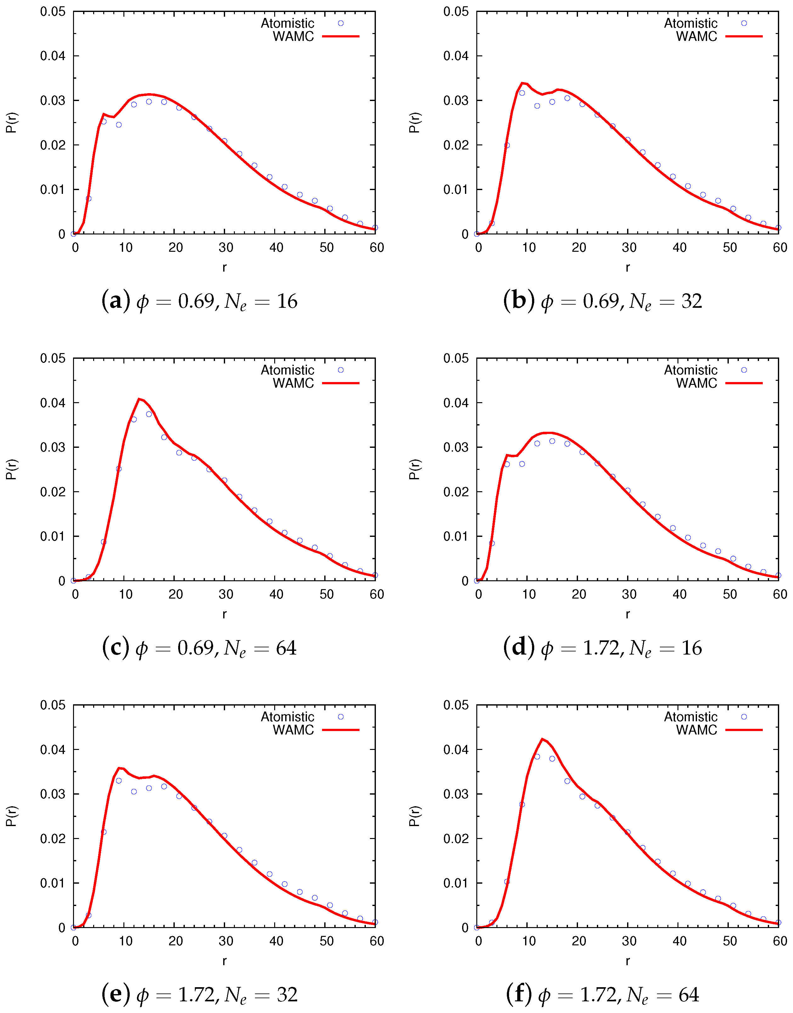
Figure 9 compares the intra-segment distribution functions for ϕ = 0 . 69 and 1.72 using both the fully-atomistic and the coarse-grained models. It can be seen that the results from CG simulations are in good agreement with the fully-atomistic simulations for both ϕ = 0 . 69 and 1.72. Furthermore, increasing the density has no major effect on the coarse-grained distribution functions with only slight discrepancies between the two models at short distances due to the approximations introduced while computing the potentials. As discussed in the previous section, the actual intramolecular function is quite complex, and at higher densities, these approximations are likely to break down due to many-body correlations. As we move towards higher coarse-graining levels, from N e = 16–64, there is no change in the results aside from an increase in the probability of finding a segment within a chain. The agreement between the coarse-grained model with N e = 64 and the non-coarse-grained model is quite consistent.
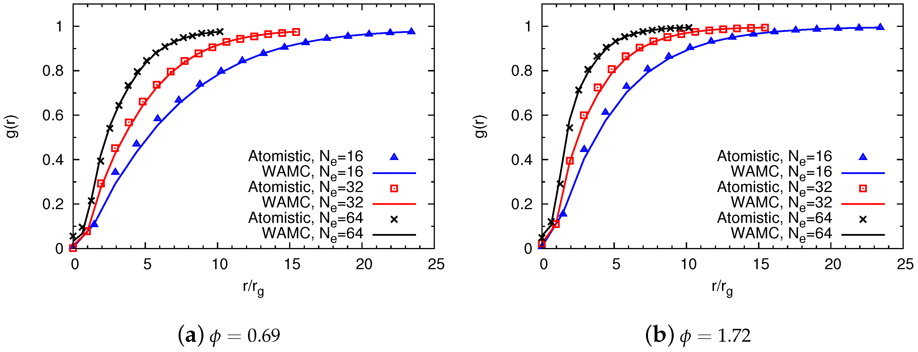
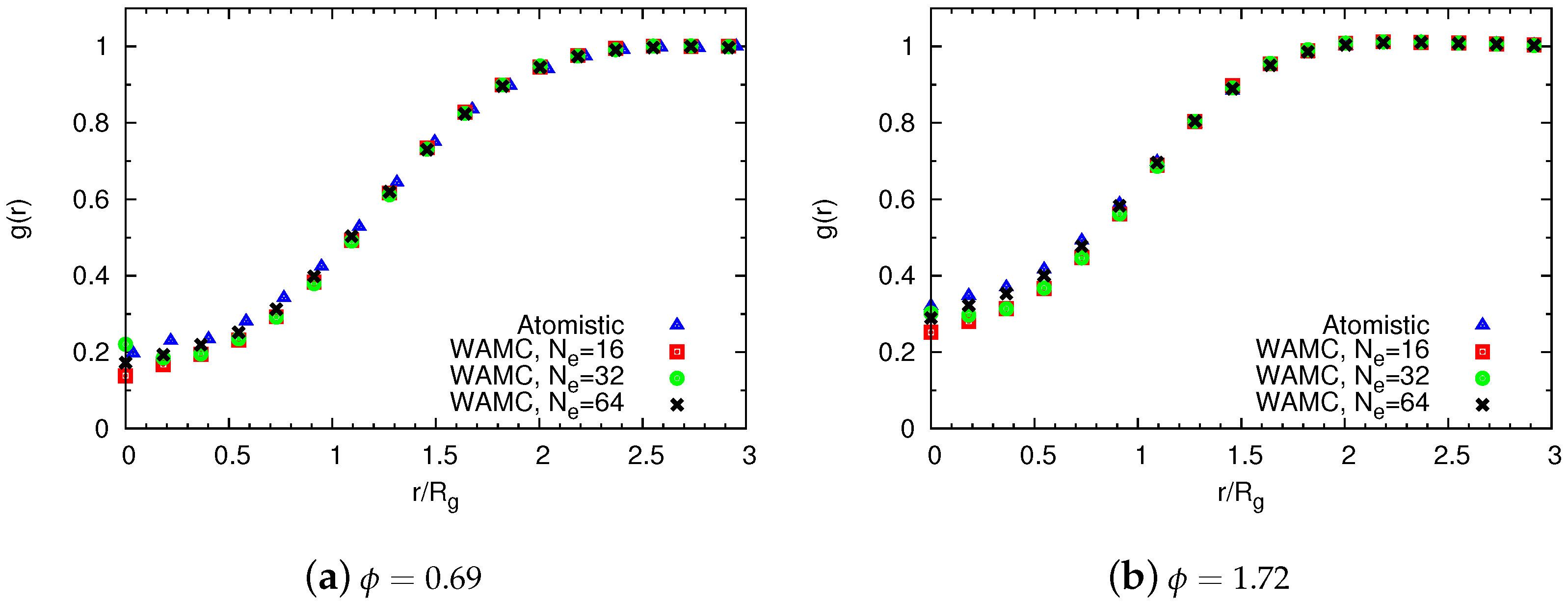
Figure 10 shows the inter-segment radial distribution functions obtained from the atomistic and with coarse-grained simulations for ϕ = 0 . 69 and 1.72. Again, the inter-segment distributions from the coarse-grained simulations are in extremely close agreement with the atomistic distribution for all values of N e , showing that the coarse-grained model reproduces the center-of-mass pair correlation functions obtained from atomistic model with great precision. This further justifies the use of the intermolecular potential as the potential of mean force between two polymer chains of size N e at these densities. Provided that the entropic contribution to the free energy of this interaction is negligible, this can be used as the intermolecular potential between the coarse-grained beads of different chains. These findings are in agreement with the results obtained by Pierleoni et al. [37,38], who found that many-body correlations are absent provided that the coarse-grained bead density is below the overlap density of the coarse-grained beads.
The results of the intra-segment distributions and inter-segment RDF’s prove that the allowed moves in the coarse-grained simulation adequately sample the phase space of the underlying atomistic model. Furthermore, the CG force field is clearly transferable to different densities. It should be noted that we have only sampled a single freely-jointed chain to obtain the probability distributions used to simulate semidilute solutions at different resolutions. The center-of-mass radial distribution functions are shown in Figure 11. This result is of considerable importance as the center-of-mass radial distribution function can be used to obtain the second virial coefficient of the system. The figure shows that there is a satisfactory agreement between the atomistic and coarse-grained systems. As the density of the system increases, however, the assumption breaks down, and discrepancies at low r / r g begin to appear, as shown in Figure 11b.
Table 4 shows the average radius of gyration obtained from the atomistic and coarse-grained simulations. In the zero-density limit, the radius of gyration of a chain with N = 512 monomers obtained is 20.2. As the density of polymer chains increases, the average radius of gyration of a single chain decreases due to additional correlations with the other chains. This reduction in the radius of gyration is captured precisely in the coarse-grained model at all resolutions. As discussed in the previous section, however, the coarse-grained values will be slightly underestimated when compared with the atomistic results.

5. Conclusions and Outlook

We have extended the wavelet-accelerated Monte Carlo approach to a semi-dilute system of polymer chains under athermal conditions. It was demonstrated that such a coarse-graining scheme is effective and that one can access different length scales conveniently within a single computational routine. The bonded and non-bonded potentials were obtained from zero density simulations, which were then parameterized using different scaling factors. This enables one to use the same potential functions at each of the different simulation scales, circumventing the need for recalculation when moving from one scale to the next.
To extend the wavelet transform approach to semidilute system of polymer chains, a significant approximation was made in which the intermolecular potential was assumed to be equal to the non-bonded potential. We show that this approximation is quite reasonable provided that the coarse-grained bead density is below the overlap density of the coarse-grained beads. Thus, using the results of the single chain statistics, we are able to simulate semidilute systems at different densities and length scales. The results from the coarse-grained and atomistic simulations were compared and showed that the coarse-grained polymer systems can reproduce results to a reasonable degree of accuracy.
Future works might extend the above approach for polymer solutions in concentrated regimes. The major challenge here would be to compute intermolecular potentials that are “universal” and can be transferred to different densities. One option would be to use the iterative Boltzmann inversion (BI) approach to derive an effective coarse-grained potential for a given (nonzero) density. Then, at each coarse-grained stage, one could use the potential from the previous stage as the starting approximation and then perform a few additional BI iterations to reach the final potential at that particular resolution. A somewhat similar method known as multi-state iterative Boltzmann inversion was developed by McCabe et al. [40]. One can also introduce a reverse-mapping scheme within the WAMC framework in precisely the same way. Using the probability distributions for the bond, angle, dihedral and non-bonded terms obtained during the coarse-graining procedure, one can reconstruct the fine details of the polymer that are consistent with both the geometric constraints and energetic considerations.
We would also like to extend the method to study chain dynamics using molecular dynamics simulations. The recent work by Hsu et al. [41,42], which shows that parameterizing non-bonded interactions allow for the good approximation of chain dynamics, could be used as the basis for such a study.

Acknowledgments

We are thankful to the high-performance computing service at RWTHAachen for providing the computational resources.

Author Contributions

Animesh Agarwal performed the computations, and all the authors developed the idea. Animesh Agarwal and Ahmed E. Ismail designed the research plan, and all the authors wrote the paper.

Conflicts of Interest

The authors declare no conflict of interest.

Appendix A. Validity of Using Zero-Density Potentials for the Intermolecular Potential

The concentration of polymer chains is
ρ b = M V ,
and the overlap concentration is
ρ * = 3 4 π R g 3 ,
where R g = b N ν is the radius of gyration. The semidilute regime exists when
ϕ = ρ b ρ * = 4 π M R g 3 3 V > 1 .
We can think of this system as composed of superatoms or coarse-grained beads, where the local bead density permits use of the non-bonded potential as the inter-chain potential. If a chain of L monomers is partitioned into N b CG beads with N e monomers per bead, the local concentration of the beads is
ρ C G , b = M N b V ,
and the bead overlap concentration is given by
ρ CG * = ρ * = 3 4 π R g 3 .
If the radius of gyration is taken to be R g = b N e ν , where b is the Kuhn length that appears in the scaling of radius of gyration, then:
ϕ CG = ρ C G , b ρ CG * = M N b 4 π b 3 N e 3 ν 3 V
and therefore
ϕ CG ϕ = N b b 3 N e 3 ν b 3 N 3 ν = N b N e N 3 ν = N b 1 3 ν .
Thus,
ϕ CG = ϕ N b 1 3 ν .
For athermal and good solvents, the Flory exponent ν 0 . 588 . Upon substitution in the above equation, this yields:
ϕ CG = ϕ N b 0 . 76
Thus for any polymer volume fraction ϕ > 1 which is a semidilute regime, N b can be chosen such that the coarse-grained bead overlap volume fraction ϕ CG < 1 , and hence the beads do not overlap. It is therefore reasonable to neglect many-body interactions among the coarse-grained beads and to represent intermolecular interactions by the zero-density pair potential. Thus, the total energy now becomes:
U t o t a l = i = 1 M U i n t r a + i = 1 M 1 a = 1 N b j = i + 1 M b = 1 N b ϕ n b .

References

  1. Akkermans, R.; Briels, W. Coarse-grained interactions in polymer melts: A variational approach. J. Chem. Phys. 2001, 115, 6210–6219. [Google Scholar] [CrossRef]
  2. Baschnagel, J.; Binder, K.; Doruker, P.; Gusev, A.; Hahn, O.; Kremer, K.; Mallice, W.; Muller-Plathe, F.; Murat, M.; Paul, W.; et al. Bridging the gap between atomistic and coarse-grained models of polymers: Status and perspectives. Adv. Polym. Sci. 2000, 152, 41–156. [Google Scholar]
  3. Lyubarstev, A.; Karttunen, M.; Vattulainen, I.; Laaksonen, A. On coarse-graining by the inverse Monte Carlo method: Dissipative particle dynamics simulations made to a precise tool in soft matter modeling. Soft Matter 2003, 1, 121–137. [Google Scholar]
  4. Tan, R.; Petrov, A.; Harvey, S. YUP: A molecular simulation program for coarse-grained and multi-scaled models. J. Chem. Theory Comput. 2006, 2, 529–540. [Google Scholar] [CrossRef] [PubMed]
  5. Clementi, C. Coarse-grained models of protein folding: Toy models or predictive tools? Curr. Opin. Struct. Biol. 2008, 18, 10–15. [Google Scholar] [CrossRef] [PubMed]
  6. Ashbaugh, H.; Patel, H.; Kumar, S.; Garde, S. Mesoscale model of polymer melt structure: Selt consistent mapping of molecule correlations to coarse-grained potentials. J. Chem. Phys. 2005, 122. [Google Scholar] [CrossRef] [PubMed]
  7. Fukunaga, H.; Takimoto, J.; Doi, M. A coarse-graining procedure for flexible polymer chains with bonded and nonbonded interactions. J. Chem. Phys. 2002, 116, 8183–8190. [Google Scholar] [CrossRef]
  8. Harmandaris, V.; Adhikari, N.; Van der Vegt, N.; Kremer, K. Heirarchical modeling of polystyrene: From atomistic to coarse-grained simualtions. Macromolecules 2006, 39, 6708–6719. [Google Scholar] [CrossRef]
  9. Kamio, K.; Moorthi, K.; Theodorou, D. Coarse grained end bridging Monte Carlo simulations of poly(ethylene terephthalate) melt. Macromolecules 2007, 49, 710–722. [Google Scholar] [CrossRef]
  10. Pandiyan, S.; Parandekar, P.V.; Prakash, O.; Tsotsis, T.K.; Basu, S. Systematic coarse graining of a high-performance polyimide. Macromol. Theory Simul. 2015, 24, 513–520. [Google Scholar] [CrossRef]
  11. Lyubartsev, A.P.; Naome, A.; Vercauteren, D.P.; Laaksonen, A. Systematic hierarchical coarse-graining with the inverse Monte Carlo method. J. Chem. Phys. 2015, 143. [Google Scholar] [CrossRef] [PubMed]
  12. Yang, D.; Wang, Q. Systematic and simulation-free coarse graining of homopolymer melts: A relative-entropy-based study. Soft Matter 2015, 11, 7109–7118. [Google Scholar] [CrossRef] [PubMed]
  13. Yang, D.; Wang, Q. Systematic and simulation-free coarse graining of homopolymer melts: A structure-based study. J. Chem. Phys. 2015, 142. [Google Scholar] [CrossRef] [PubMed]
  14. Zhang, G.; Moreira, L.A.; Stuehn, T.; Daoulas, K.C.; Kremer, K. Equilibration of high molecular weight polymer melts: A hierarchical strategy. ACS Macro Lett. 2014, 3, 198–203. [Google Scholar] [CrossRef]
  15. Ismail, A.E.; Rutledge, G.C.; Stephanopoulos, G. Topological coarse-graining of polymer chains using wavelet-accelerated Monte Carlo. I. Freely jointed chains. J. Chem. Phys. 2005, 122. [Google Scholar] [CrossRef] [PubMed]
  16. Ismail, A.E.; Rutledge, G.C.; Stephanopoulos, G. Topological coarse-graining of polymer chains using wavelet-accelerated Monte Carlo. II. Self-avoiding chains. J. Chem. Phys. 2005, 122. [Google Scholar] [CrossRef] [PubMed]
  17. Ismail, A.E.; Rutledge, G.C.; Stephanopoulos, G. Multiresolution analysis in statistical mechanics. I. Using wavelets to calculate thermodynamic properties. J. Chem. Phys. 2003, 118. [Google Scholar] [CrossRef]
  18. Ismail, A.E.; Stephanopoulos, G.; Rutledge, G.C. Multiresolution analysis in statistical mechanics. II. The wavelet transform as a basis for Monte Carlo simulations on lattices. J. Chem. Phys. 2003, 118. [Google Scholar] [CrossRef]
  19. Rinderspacher, B.; Bardhan, J.; Ismail, A. Theory of wavelet-based coarse-graining hierarchies for molecular dynamics. Phys. Rev. E 2017, 96. [Google Scholar] [CrossRef]
  20. Chen, J.; Teng, H.; Nakano, A. Wavelet-based multi-scale coarse graining approach for DNA molecules. Finite Elem. Anal. Des. 2007, 43, 346–360. [Google Scholar] [CrossRef]
  21. Maiolo, M.; Vancheri, A.; Krause, R.; Danani, A. Wavelets as basis functions to represent the coarse-graining potential in multiscale coarse graining approach. J. Comput. Phys. 2015, 300, 592–604. [Google Scholar] [CrossRef]
  22. Praprotnik, M.; Delle Site, L.; Kremer, K. Adaptive resolution molecular-dynamics simulation: Changing the degrees of freedom on the fly. J. Chem. Phys. 2005, 123. [Google Scholar] [CrossRef] [PubMed]
  23. Wang, H.; Hartmann, C.; Schütte, C.; Delle Site, L. Grand-canonical-like molecular-dynamics simulations by using an adaptive-resolution technique. Phys. Rev. X 2013, 3. [Google Scholar] [CrossRef]
  24. Daubechies, I. Ten lectures on wavelets. In CBMS-NSF Regional Conference Series in Applied Mathematics: Ten Lectures on Wavelets No. 61 by Ingrid Daubechies; Society for Industrial and Applied Mathematics: Philadelphia, PA, USA, 1992. [Google Scholar]
  25. Strang, G.; Nguyen, T. Wavelets and Filter Banks; Wellesley-Cambridge Press: Wellesley, MA, USA, 1996. [Google Scholar]
  26. Haar, A. Zur Theorie der orthogonalen Funktionensysteme, (Erste Mitteilung). Math. Ann. 1910, 69, 331–369. [Google Scholar] [CrossRef]
  27. Muller-Plathe, F. Coarse-graining in polymer simulation: From the atomistic to the mesoscopic scale and back. Chem. Phys. Chem. 2002, 3, 754–769. [Google Scholar] [CrossRef]
  28. Lal, M. ‘Monte Carlo’ computer simulations of chain molecules. Mol. Phys. 1969, 17, 57–64. [Google Scholar] [CrossRef]
  29. Dickman, R.; Hall, C. Equation of state for chain molecules: Continuous space analog of Flory theory. J. Chem. Phys. 1986, 85. [Google Scholar] [CrossRef]
  30. Metropolis, N.; Rosenbluth, A.W.; Rosenbluth, M.N.; Teller, A.H.; Teller, E. Equation of state calculations by fast computing machines. J. Chem. Phys. 1953, 21, 1087–1092. [Google Scholar] [CrossRef]
  31. Peter, C.; Kremer, K. Multiscale simulation of soft matter systems-from the atomistic to the coarse-grained level and back. Soft Matter 2009, 5, 4357–4366. [Google Scholar] [CrossRef]
  32. Bolhuis, P.; Louis, A.; Hansen, J.; Meijer, E. Accurate effective pair potentials for polymer solutions. J. Chem. Phys. 2001, 114, 4296–4311. [Google Scholar] [CrossRef]
  33. Bolhuis, P.; Louis, A.; Hansen, J. Many-body interactions and correlations in coarse-grained descriptions of polymer solutions. Phys. Rev. E 2001, 64. [Google Scholar] [CrossRef] [PubMed]
  34. Dautenhahn, J.; Hall, C. Monte Carlo simulation of off-lattice polymer chains: Effective pair potentials in dilute solution. Macromolecules 1994, 27, 5399–5412. [Google Scholar] [CrossRef]
  35. Kremer, K.; Binder, K. Monte Carlo simulation of lattice models for macromolecules. Comput. Phys. Rep. 1988, 7, 259–310. [Google Scholar] [CrossRef]
  36. Lyubartsev, A.; Laaksonen, A. Calculation of effective interaction potentials from radial distribution functions: A reverse Monte Carlo approach. Phys. Rev. E 1995, 52, 3730–3737. [Google Scholar] [CrossRef]
  37. D’Adamo, G.; Pelissetto, A.; Pierleoni, C. Coarse-grained strategies in polymer solutions. Soft Matter 2012, 8, 5151–5167. [Google Scholar] [CrossRef]
  38. D’Adamo, G.; Pelissetto, A.; Pierleoni, C. Consistent and transferable coarse-grained model for semidilute polymer solutions in good solvent. J. Chem. Phys. 2012, 137. [Google Scholar] [CrossRef] [PubMed]
  39. Kumar, S.; Vacatello, M.; Yoon, D. Offlattice Monte Carlo simulations of polymer melts confined between two plates. J. Chem. Phys. 1988, 89. [Google Scholar] [CrossRef]
  40. Moore, T.; Iacovella, C.; McCabe, C. Derivation of coarse-grained potentials via multistate iterative Boltzmann inversion. J. Chem. Phys. 2014, 140. [Google Scholar] [CrossRef] [PubMed]
  41. Hsu, D.; Xia, W.; Arturo, S.; Keten, S. Systematic method for thermomechanically consistent coarse-graining: A universal model for methacrylate-based polymers. J. Chem. Theory Comput. 2014, 10, 2514–2527. [Google Scholar] [CrossRef] [PubMed]
  42. Hsu, D.; Xia, W.; Arturo, S.; Keten, S. Thermomechanically consistent and temperature transferable coarse-graining of atactic polystyrene. Macromolecules 2015, 48, 3057–3068. [Google Scholar] [CrossRef]
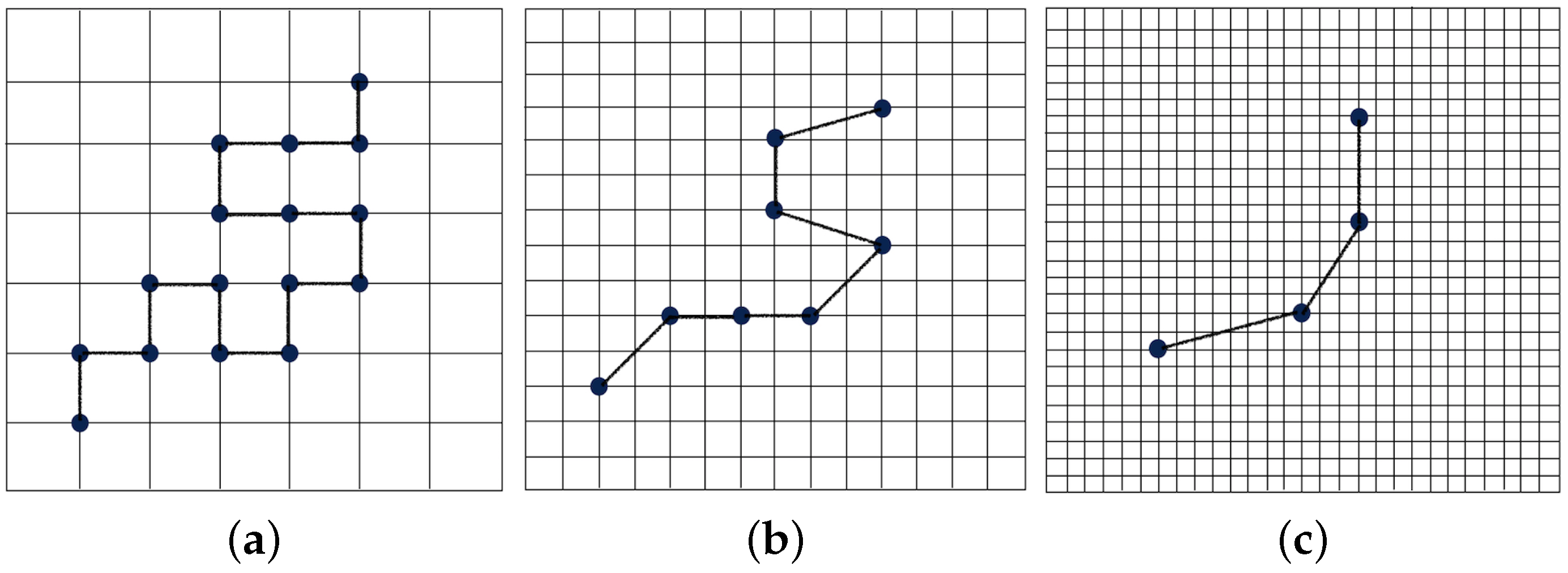
Figure 1. Coarse-graining of a random walk in two dimensions using the wavelet-transform method. (a) Random walk on a lattice representing the “atomistic” polymer chain ( N e , 1 = 1 and N b , 1 = 16 ); (b) coarse-grained chain after one level of coarse-graining ( N e , 2 = 2 and N b , 2 = 8 ); (c) coarse-grained chain after two levels of coarse-graining ( N e , 3 = 4 and N b , 3 = 4 ). N e , k corresponds to the No. of beads in the full-atomistic chain that are coarse-grained, and N b , k corresponds to the total No. of beads at the k-th simulation level. Although the figure shows the application of the wavelet transform on a lattice, our simulations are performed off-lattice.
Computation 05 00044 g001
Figure 2. Schematic representation of the original WAMC method.
Computation 05 00044 g002
Figure 3. Non-bonded potential U ( r ) for CG beads of size N e = 32 , N e = 64 and N e = 128 .
Computation 05 00044 g003
Figure 4. “Universal” functions for the CG non-bonded potential. (a) Coarse-grained non-bonded potential obtained from chains of length N e = 32 , 64 and 128, with distance normalized by the radius of gyration R g ; (b) Collapse of coarse-grained non-bonded potential obtained from chains of length N e = 32 , 64 and 128 showing an N e 0 . 19 dependence on the magnitude of the potential.
Computation 05 00044 g004
Figure 5. Variance in the potential U ( 0 ) for chains with N e = 32 , 64 and 128 as a function of the exponent ζ used to fit a scaling relation of the form N e ζ .
Computation 05 00044 g005
Figure 6. Distribution functions between the CG beads of size N e = 32, 64 and 128 required for reverse Monte Carlo. (a) Bond-length distributions; (b) bond-angle distributions for r < 1 . 5 N e 1 / 2 ; (c) bond-angle distributions for r > 1 . 5 N e 1 / 2 ; (d) torsion-angle distributions; (e) 1–2 neighbor distributions; (f) 1–3 neighbor distributions; (g) 1–4 neighbor distributions.
Computation 05 00044 g006
Figure 7. Potentials for bonded interactions between (a) 1–2 neighbors, (b) 1–3 neighbors and (c) 1–4 neighbors, as obtained from nine iterations of reverse Monte Carlo. Simulation results are shown in black, polynomial fits in red.
Computation 05 00044 g007
Figure 8. Schema of the modified WAMC algorithm.
Computation 05 00044 g008
Figure 9. Intra-segment distribution functions showing the comparison between atomistic and coarse-grained models: for ϕ = 0 . 69 with (a) N e = 16 ; (b) N e = 32 ; (c) N e = 64 ; and ϕ = 1 . 72 with (d) N e = 16 ; (e) N e = 32 ; and (f) N e = 64 .
Computation 05 00044 g009
Figure 10. Inter-segment RDF’s showing the comparison between atomistic and coarse-grained models for (a) ϕ = 0 . 69 and (b) ϕ = 1 . 72 .
Computation 05 00044 g010
Figure 11. Center-of-mass RDF’s showing the comparison between atomistic and coarse-grained models for (a) ϕ = 0 . 69 and (b) ϕ = 1 . 72 .
Computation 05 00044 g011
Table 1. Radius of gyration for polymer chains of different lengths calculated using the atomistic model and coarse-grained model under two levels of coarse-graining, for ϵ / k B T = 0 . 0 , 0 . 10 and 0 . 15 .
N ϵ / k B T = 0 . 0 ϵ / k B T = 0 . 10 ϵ / k B T = 0 . 15
N e = 1 N e = 32 N e = 64 N e = 1 N e = 32 N e = 64 N e = 1 N e = 32 N e = 64
256177184165143142139133132125
512410422378322325316298299283
1024957990916755759716659697641
2048219822832130173217371657149315911481
4096505251514895397339323772358336183373
819211,76711,85811,243900689358548786480707613
16,38427,18427,24026,19020,66220,46819,50017,81818,28217,249
32,76862,79962,58261,00947,40446,89344,49040,37041,42439,083
Table 2. Flory exponent obtained using atomistic and coarse-grained models.
ϵ / k B T ν
AtomisticCG, N e = 32 CG, N e = 64
0.00.6040.6010.610
−0.100.5990.5980.595
−0.150.5900.5950.593
Table 3. Specific details of the systems studied in this work. Here, N denotes the size of a single chain, M the No. of chains and L the size of the box.
ϕ NLM
0.6951210020
1.7251210050
Table 4. Average radius of gyration obtained from the atomistic and coarse-grained system, at different polymer volume fractions ϕ .
Model
2–5 ϕ AtomisticCG, N e = 16 CG, N e = 32 CG, N e = 64
0.020.2320.0819.8719.57
0.6917.1216.9816.7516.59
1.7216.6116.2416.0415.98