Analytical Results on the Behavior of a Liquid Junction across a Porous Diaphragm or a Charged Porous Membrane between Two Solutions According to the Nernst–Planck Equation

Abstract

We model the behavior of an ideal liquid junction, across a porous and possibly charged medium between two ion-containing solutions, by means of the Nernst–Planck equation for the stationary state, in conditions of local electroneutrality. An analytical solution of the equation was found long ago by Planck for the uncharged junction with only ions of valences +1 and −1. Other analytical results, which have later been obtained also for more general situations, seem impractical for performing calculations. In this paper, we obtain analytical solutions for systems with up to three valence classes, which can be applied to perform numerical calculations in a straightforward way. Our method provides a much larger amount of information on the behavior of the system than the well-known Henderson’s approximation. At the same time, it is more simple and reliable, and much less demanding in terms of computational effort, than the nowadays commonly employed numerical methods, typically based on discrete integration and trial-and-error numerical inversions. We present some examples of practical applications of our results. We study in particular the uphill transport (i.e., the transport from the lower-concentration to the higher-concentration region) of a divalent cation in a liquid junction containing also other univalent anions and cations.

1. Introduction

When two solutions of different electrolytes, or of the same electrolyte but with different concentrations, are put into contact, a potential, called “liquid junction potential”, spontaneously arises between them [1]. Such a potential develops for instance across the porous diaphragm of concentration cells, thus affecting the output potential, and across the diaphragm of the reference electrodes which are commonly used in electrochemistry, thus affecting the measurements of the electrode potentials. On the other hand, since every electrochemical measurement also involves potential differences which arise between the electrodes and the solutions, a reliable experimental measurement of the liquid junction potential alone is often practically unavailable. For this reason, several methods to theoretically calculate the liquid junction potential have been conceived and employed for a long time.

An approximated formula for the junction potential, which gives results sufficiently accurate for most practical purposes, and which is for this reason largely employed still today, has been obtained by Henderson in 1907 [2,3]. A more rigorous approach to the problem had however been adopted by Planck already in 1890 [4,5]. The general behavior of an ion in an ideal liquid junction, which moves under the influence of diffusion and of an electric field, is described by the Nernst–Planck differential equation [4,5,6,7]. Planck obtained an analytical solution of this equation describing the stationary state of an uncharged liquid junction in which only univalent ions are present, under the assumption of local electroneutrality. This assumption means that the Nernst–Planck equations, for all the ionic species present in the junction, are solved with the constraint that the total electric charge vanishes at all points of the junction. In most practically relevant cases the behavior of the electric potential, which is obtained with this method, turns out to be consistent, according to the Poisson equation, with the presence of a charge density which is indeed very low compared with the charge density carried by each individual ionic species. This can be considered as a sound justification for the electroneutrality assumption.

A more rigorous procedure would be to couple the Nernst–Planck equations right from the beginning with the Poisson equation for the electric potential, without invoking electroneutrality. One obtains in this way a closed set of equations which is known as the Poisson–Nernst–Planck system. MacGillvray [8] proved that, for membranes such that the fixed charges are described by a continuum distribution, the solution of the stationary Nernst–Planck equations with electroneutrality represents the zeroth-order term of the expansion of the solution of the full Poisson–Nernst–Planck system, with respect to a parameter which is the square of the ratio of a suitable Debye length in the junction and the junction thickness. Since in practical situations such a parameter is typically very small, this argument represents a mathematically rigorous justification for the use of the electroneutrality condition.

From Planck’s solution, an analytical expression for the potential and the ionic fluxes can be derived. Planck considered a junction with well-defined spatial boundaries, corresponding for instance to the walls of a porous diaphragm between the solutions. The same situation will be considered in the present paper, and is often referred to in modern literature as the “constrained junction”, to distinguish it from the “free junction” which establishes between two solutions when they are simply in contact with one another without any physical separation between them [9]. For ideal junctions the diffusion and mobility coefficients D and μ of each ion are assumed to be constant parameters related to one another by Einstein’s relation D = μkT. For real solutions these conditions are usually approximately satisfied only for low concentrations: in the general case, the dependence of D and μ on the ion concentrations ought to be taken into account.

The Nernst–Planck equation can also be applied to describe the diffusion of ions inside a charged membrane, which can be considered as a porous medium with fixed electric charges. The simplest way to do so is to include in the model a fixed uniform charge density. Membranes have become increasingly important over the years in several technological domains, thanks to their capability to favor the exchange between two solutions of ions with a definite sign, namely the opposite one with respect to the fixed charges [10]. Membranes are also largely studied in connection with the research on nanopores and biological ion channels.

After Planck, several other authors have applied the Nernst–Planck equation to the theoretical study of liquid junctions and charged membranes [11,12,13,14]. In 1954 Schlögl [15] obtained a general analytical solution for a (possibly) charged membrane with arbitrary numbers of ionic species and ionic valences. His formulas are however rather cumbersome and contain parameters which are determined by implicit relations which are impractical to use for numerical computations. For these reasons Schlögl’s work, although occasionally mentioned in advanced textbooks [10], is today essentially neglected in the praxis of scientific research.

Several years later Morf [16] has considered again the problem with ions of only two different valences, providing a new interesting derivation of Planck’s old result, which applies also to the case in which the two valences—a single one for all the cations and another one for all the anions—are arbitrary and not necessarily +1 and −1.

In more recent times, solutions of the Nernst–Planck equations for liquid junctions and membranes have been mainly obtained by means of finite difference numerical integrations, and the development of computers has made possible to treat with these methods a much wider class of situations, including the time-dependent case [17,18,19,20,21]. Several works have also been devoted to the determination of numerical solutions of the full Poisson–Nernst–Planck system. This approach has been used to study the behavior of liquid junctions and membranes in various scientific contexts [9,22,23,24,25,26,27,28,29,30], and in particular in the study of the ions flow across biological cells [31,32,33,34,35,36,37,38,39]. More specifically, the problem of liquid junction potentials has received careful consideration owing to its importance for the correct interpretation of electrophysiological measurements [40].

In the present paper we shall study the Nernst–Planck equations in conditions of local electroneutrality, and we shall present a new analytical method of solution which extends Planck’s results by considering the presence of a fixed charged background and of mobile ions of arbitrary valences. Our main result is that a complete analytical solution can be obtained for an ideal junction across a possibly charged porous diaphragm containing ions with up to three different valences, in the presence of an arbitrary electric current. We obtain in this way, as functions of the total current, the ionic fluxes and the potential difference between the two sides of the junction or membrane, as well as the profiles of the ion concentrations and of the electric potential across the diffusion layer. These results can in particular be applied to the calculation of the potential and ionic fluxes through a diffusion layer between the solutions of two generic binary salts having an ion in common. An interesting phenomenon which can also be described is the uphill transport of a divalent cation (i.e., the transport of the ion against its concentration gradient) driven by the liquid junction or membrane potential at open circuit.

For more than three valence classes the differential equations that we obtain can be integrated with a numerical computer program. A new open source applet to perform these calculations in the case of a liquid junction at zero current has been recently made publicly available on the web [41,42]. This applet also allows considering nonideal junctions for which an analytical dependence of the ion mobilities on the concentrations can be provided.

The paper is organized as follows. In Section 2 we explain the physical assumptions at the basis of the model of liquid junction and charged membrane here considered, and recall the Nernst–Planck equations for the ion concentrations in the stationary state. In Section 3, by a change of variables in the Nernst–Planck equations, we obtain a closed system of differential equations, containing a suitable set of independent parameters which can be determined from the available information on the system, namely the ion concentrations at the two edges of the diffusion layer and the total current density. In Section 4 and Section 5 we show that this system of differential equations can be analytically solved for systems with two and three different ionic species, and obtain explicit formulas ready for use in practical applications. In Section 6 we show how our procedure can be generalized to the case in which more than three ionic species are present, as far as they do not belong to more than three different valence classes. In Section 7 we present and discuss the results which are obtained with our method in particular cases, and show that they allow the study of phenomena which are not described by Henderson’s simplified model. Finally, the conclusions of the paper are summarized in Section 8.

2. Definition of the Problem

We assume that n ion species are present inside the diffusion layer, with concentrations c_i, i = 1, …, n, expressed as number of ions per unit volume, and therefore proportional to the molar concentration. We assume that the system has a planar symmetry, so that the concentrations depend only on one spatial coordinate x varying from x = 0 to x = L, where L is the thickness of the diffusion layer. The ion fluxes Φ_i (number of ions per unit time per unit area) satisfy the Nernst–Planck equations

$${\Phi }_i=-D_i\frac{\partial c_i}{\partial x}-e{z}_i{\mu }_i{c}_i\frac{\partial V}{\partial x}i=1,\dots ,n$$

(1)

where D_i is the diffusion coefficient of the ion, z_i is its relative charge, μ_i the mobility of the ion in the solution (defined as the ratio between the drift velocity and the total acting force), e the (positive) elementary charge, and V the electric potential. Since charged membranes and—in most cases—also liquid junctions physically consist of porous materials, in the definition of ion fluxes one has to consider an effective area which represents only the porous fraction of the geometrical cross section of the diffusion layer. The numerical value of such a fraction of course depends on the particular material considered, and will not be included in the calculations and in the results which will be presented in the present paper. It can however easily be introduced in the final formulas, whenever this is required for practical applications.

The diffusion coefficient D_i and the mobility μ_i generally depend on the concentrations. However they can be considered approximately constant for very low concentrations, or when the concentrations at the two edges of the diffusion layer are similar. Furthermore, for low concentrations one can apply Einstein’s relation D_i = μ_ikT, where k is the Boltzmann constant and T the absolute temperature. Here however we shall make no use of Einstein’s relation and we shall treat D_i and μ_i as two constants such that μ_i = η_iD_i/kT, where η_i a dimensionless coefficient not necessarily equal to 1.

The concentration c_i and the flux Φ_i are connected to each other also by the continuity equation ∂Φ_i/∂x + ∂c_i/∂t = 0. If we assume that the junction has reached a stationary state, all time derivatives vanish. Hence the continuity equation implies that the ionic fluxes are independent both of time and of the position inside the junction. If we introduce the ionic charge densities (divided by e) ρ_i = z_ic_i, the constants χ_i = z_iΦ_i/D_i, and the dimensionless potential φ = eV/kT, Equation (1) can be written as

$$\frac{d{\rho }_i}{dx}=-{\chi }_i-{\zeta }_i{\rho }_i\frac{d\varphi }{dx}i=1,\dots ,n$$

(2)

with ζ_i = η_jz_j (hence ζ_i = z_i when Einstein’s relation is used).

In most practical situations a condition of local electroneutrality is satisfied inside the junction with very good approximation, so that we can assume that the equation

$${\displaystyle \sum _{i=1}^n}{\rho }_i\left(x\right)+{\rho }_0=0$$

(3)

is almost exactly satisfied at all points x. In this formula ρ₀ is a constant such that eρ₀ represents a charge density due to the presence of fixed charges uniformly distributed throughout a membrane. For the case of liquid junctions one has simply to put ρ₀ = 0 here and in all the equations that follow. As a consequence of Equation (3) we can treat only ${\rho }_1,\dots ,{\rho }_{n-1}$ as independent charge densities, while ${\rho }_n=-{\sum }_{i=1}^{n-1}{\rho }_i-{\rho }_0$.

Let us denote with a prime all physical quantities evaluated at the edge x = 0 of the diffusion layer, and with a double prime the same quantities evaluated at the edge x = L. So, for instance, $V^{\prime }=V\left(0\right)$, $V^{″}=V\left(L\right)$, ${\rho }_1^{\prime }={\rho }_1\left(0\right)$, ${\rho }_1^{″}={\rho }_1\left(L\right)$, etc. Assuming that the ion concentrations at the two edges of the diffusion layer—i.e., ${\rho }_1^{\prime },\dots ,{\rho }_n^{\prime }$, ${\rho }_1^{″},\dots ,{\rho }_n^{″}$—are known, our goal is to determine the dependence of the potential difference $\Delta V=V^{″}-V^{\prime }$ between the two edges, on the total current density

$$J={\displaystyle \sum _{i=1}^n}e{z}_i{\Phi }_i$$

(4)

flowing through the liquid junction. In addition, for any arbitrary point of the J–ΔV curve we aim to fully characterize the stationary state of the junction by determining the fluxes ${\Phi }_i$ of the individual ionic species and their densities ${\rho }_i\left(x\right)$ as functions of the position x, together with the behavior of the potential $V\left(x\right)$ across the diffusion layer.

In the case of the uncharged liquid junction, i.e., for ${\rho }_0=0$, the concentrations of the ions at the two edges of the junction are the same as those inside the solutions A and B at the two corresponding sides: $c_i^{\prime }=c_i^A$ and $c_i^{″}=c_i^B$. Moreover, each of the two solutions is at the same potential as the neighbouring boundary of the junction, i.e., $V^A=V^{\prime }$ and $V^B=V^{″}$. Hence the potential difference $V_{\text{ext}}=V^B-V^A$ between the two solutions is the same as the potential difference $\Delta V=V^{″}-V^{\prime }$ between the two boundaries: $V_{\text{ext}}=\Delta V$.

In the case of the charged membrane instead, the concentrations at the edges of the membrane do not coincide with the concentrations in the two solutions, since for the neutrality conditions respectively in the membrane and in the solutions we have

$$\begin{array}{c}\hfill {\displaystyle \sum _{i=1}^n}{\rho }_i^{\prime }={\displaystyle \sum _{i=1}^n}{\rho }_i^{″}=-{\rho }_0\end{array}$$

(5)

$$\begin{array}{c}\hfill {\displaystyle \sum _{i=1}^n}{\rho }_i^A={\displaystyle \sum _{i=1}^n}{\rho }_i^B=0\end{array}$$

(6)

where ${\rho }_i^A=z_i{c}_i^A$, ${\rho }_i^B=z_i{c}_i^B$. Correspondingly, in order to obtain the full potential difference $V_{\text{ext}}$ between the solutions at the two sides of the membrane, one has to respectively add and subtract to the voltage $\Delta V=V^{″}-V^{\prime }$ the Donnan potentials $V_D^A=V^{\prime }-V^A$ and $V_D^B=V^{″}-V^B$ which arise at the two boundaries of the membrane:

$$V_{\text{ext}}=\Delta V+V_D^A-V_D^B$$

The Donnan potentials are related to the ion concentrations at the two boundaries by the Donnan equilibrium relations [43]

$$\begin{array}{c}\hfill {\rho }_i^{\prime }=k_i{\rho }_i^A{e}^{-z_{i}e{V}_D^A/kT}i=1,\dots ,n\end{array}$$

(7)

$$\begin{array}{c}\hfill {\rho }_i^{″}=k_i{\rho }_i^B{e}^{-z_{i}e{V}_D^B/kT}i=1,\dots ,n\end{array}$$

(8)

where $k_i$ are the partition coefficients. From Equation (5) one then obtains

$$\begin{array}{c}\hfill {\displaystyle \sum _{i=1}^n}{k}_i{\rho }_i^A{e}^{-z_{i}e{V}_D^A/kT}=-{\rho }_0\end{array}$$

(9)

$$\begin{array}{c}\hfill {\displaystyle \sum _{i=1}^n}{k}_i{\rho }_i^B{e}^{-z_{i}e{V}_D^B/kT}=-{\rho }_0\end{array}$$

(10)

When the ion concentrations $c_1^A,\dots ,c_n^A,c_1^B,\dots ,c_n^B$ in the two solutions are known, by solving these equations one can determine $V_D^A$ and $V_D^B$. Then the ion concentrations at the two boundaries can be computed using Equations (7) and (8). A rigorous justification of the use of the Donnan equilibrium relations was given by MacGillvray [8], who proved that they lead to a good approximation of the solution of the full Poisson–Nernst–Planck system of equations for the membrane, under the same conditions which justify the use of the electroneutrality condition.

3. Mathematical Procedure

We assume the fixed charges to be uniformly distributes throughout the junction, so that $d{\rho }_0/dx=0$. By summing the Equation (2) over i we thus obtain

$$-\frac{d\varphi }{dx}=\frac{X}{{\sum }_{j=1}^n{\zeta }_j{\rho }_j}$$

(11)

where $X={\sum }_{i=1}^n{\chi }_i$. Multiplying Equation (2) by dx and using Equation (11), we then obtain

$$d{\rho }_i=d\varphi \left(h_i{\displaystyle \sum _{j=1}^n}{\zeta }_j{\rho }_j-{\zeta }_i{\rho }_i\right)$$

(12)

where $h_i={\chi }_i/X$.

It is useful here to introduce the new variables

$${\tau }_i={\rho }_i+\frac{h_i/{\zeta }_i}{{\sum }_{k=1}^n{h}_k/{\zeta }_k}{\rho }_0$$

(13)

which satisfy

$${\displaystyle \sum _{i=1}^n}{\tau }_i=0$$

(14)

Note that ${\tau }_i={\rho }_i$ for ${\rho }_0=0$. Then Equation (12) can be rewritten

$$d{\tau }_i=d\varphi \left(h_i{\displaystyle \sum _{j=1}^n}{\zeta }_j{\tau }_j-{\zeta }_i{\tau }_i\right)=d\varphi \left[h_i{\displaystyle \sum _{j=1}^{n-1}}({\zeta }_j-{\zeta }_n){\tau }_j-{\zeta }_i{\tau }_i\right]$$

(15)

which for n > 2 implies

$$\frac{d{\tau }_i}{d{\tau }_{n-1}}=\frac{h_i{\sum }_{j=1}^{n-1}({\zeta }_j-{\zeta }_n){\tau }_j-{\zeta }_i{\tau }_i}{h_{n-1}{\sum }_{j=1}^{n-1}({\zeta }_j-{\zeta }_n){\tau }_j-{\zeta }_{n-1}{\tau }_{n-1}}i=1,\dots ,n-2$$

Putting

$$r_i=\frac{{\tau }_i}{{\tau }_{n-1}}\xi =log{\tau }_{n-1}$$

(16)

and using the relation

$$\frac{d{\tau }_i}{d{\tau }_{n-1}}=\frac{d\left({\tau }_{n-1}{r}_i\right)}{d{\tau }_{n-1}}=r_i+\frac{d{r}_i}{d\xi }$$

We obtain

$$\frac{d{r}_i}{d\xi }=\frac{(h_{n-1}{r}_i-h_i){\sum }_{j=1}^{n-1}({\zeta }_j-{\zeta }_n)r_j+({\zeta }_i-{\zeta }_{n-1})r_i}{-h_{n-1}{\sum }_{j=1}^{n-1}({\zeta }_j-{\zeta }_n)r_j+{\zeta }_{n-1}}i=1,\dots ,n-2$$

(17)

It is possible to write down two linear relations among the parameters ${\chi }_1,\dots ,{\chi }_{n-1}$. First of all Equation (4) implies

$${\displaystyle \sum _{i=1}^n}{D}_i{\chi }_i=\frac{J}{e}$$

(18)

Furthermore, by dividing each of the Equation (2) by ${\zeta }_i$ and then summing over i, we obtain using Equation (3)

$$\frac{dw}{dx}=-{\displaystyle \sum _{i=1}^n}\frac{{\chi }_i}{{\zeta }_i}$$

(19)

with

$$w={\displaystyle \sum _{i=1}^n}\frac{{\rho }_i}{{\zeta }_i}-{\rho }_0\varphi$$

(20)

Since the right side of Equation (19) is a constant, we deduce that w is a linear function of x. Hence we can write

$$w=w^{\prime }+\frac{\Delta w}{L}x$$

(21)

and

$${\displaystyle \sum _{i=1}^n}\frac{{\chi }_i}{{\zeta }_i}=-\frac{\Delta w}{L}$$

(22)

with $\Delta w=w^{″}-w^{\prime }$, $w^{\prime }$ and $w^{″}$ being the values of w at the boundaries respectively x = 0 and x = L of the diffusion layer. From Equations (18) and (22) it follows that

$${\displaystyle \sum _{i=1}^n}\left(D_i+\frac{Y}{{\zeta }_i}\right){\chi }_i=0$$

(23)

where

$$Y=\frac{JL}{e\Delta w}$$

(24)

Let us define

$${\alpha }_i=\frac{{\chi }_i}{{\chi }_{n-1}}=\frac{h_i}{h_{n-1}}$$

(25)

As a consequence of Equation (23) and of Equation (25) we have

$${\alpha }_{n-1}=1{\alpha }_n=-{\displaystyle \sum _{i=1}^{n-1}}\frac{D_i+Y/{\zeta }_i}{D_n+Y/{\zeta }_n}{\alpha }_i$$

(26)

Therefore, calling $\beta =1/h_{n-1}$, and recalling that ${\sum }_{i=1}^n{h}_i=1$, we have

$$\beta ={\displaystyle \sum _{i=1}^n}{\alpha }_i={\displaystyle \sum _{i=1}^{n-1}}{s}_i{\alpha }_i={\displaystyle \sum _{i=1}^{n-2}}{s}_i{\alpha }_i+s_{n-1}$$

(27)

where

$$s_i=1-\frac{D_i+Y/{\zeta }_i}{D_n+Y/{\zeta }_n}$$

(28)

It follows that Equation (17) can be rewritten as

$$\frac{d{r}_i}{d\xi }=\frac{(r_i-{\alpha }_i){\sum }_{j=1}^{n-1}({\zeta }_j-{\zeta }_n)r_j+({\zeta }_i-{\zeta }_{n-1})\beta r_i}{-{\sum }_{j=1}^{n-1}({\zeta }_j-{\zeta }_n)r_j+{\zeta }_{n-1}\beta }i=1,\dots ,n-2$$

(29)

These represent a system of n − 2 differential equations in the unknown functions $r_1\left(\xi \right),\dots ,r_{n-2}\left(\xi \right)$. Note that, according to Equation (16), one has to put in Equation (29), $r_{n-1}=1$.

The system Equation (29) contains the n − 1 independent parameters ${\alpha }_1,\dots ,{\alpha }_{n-2}$ and Y, whose physical meaning is expressed by Equations (24) and (25), but which are a priori unknown in practical situations. Let us suppose that $c_{n-1}$, and therefore also ξ, varies monotonically from one side of the junction to the other. If the ion concentrations at the two edges are known, and a value of Y has been assigned, then ${\alpha }_1,\dots ,{\alpha }_{n-2}$ can be determined by imposing that the solution of Equation (29), with initial data

$$r_i\left({\xi }^{\prime }\right)=r_i^{\prime }=e^{-{\xi }^{\prime }}{\tau }_i^{\prime }i=1,\dots ,n-2$$

(30)

at ${\xi }^{\prime }=log{\tau }_{n-1}^{\prime }$, satisfies the n − 2 boundary conditions

$$r_i\left({\xi }^{″}\right)=r_i^{″}=e^{-{\xi }^{″}}{\tau }_i^{″}i=1,\dots ,n-2$$

(31)

at ${\xi }^{″}=log{\tau }_{n-1}^{″}$, where ${\tau }_i^{\prime }={\tau }_i{|}_{x=0}$, ${\tau }_i^{″}={\tau }_i{|}_{x=L}$, and

$${\tau }_i={\rho }_i+\frac{{\tilde{\alpha }}_i}{\tilde{\beta }}{\rho }_0$$

(32)

On the right-hand of this formula we put ${\tilde{\alpha }}_i=({\zeta }_{n-1}/{\zeta }_i){\alpha }_i$ and $\tilde{\beta }={\sum }_{k=1}^n{\tilde{\alpha }}_k$. Making use of Equation (26) one obtains

$$\tilde{\beta }=\frac{{\sum }_{k=1}^{n-2}\left({\tilde{D}}_n-{\tilde{D}}_k\right){\tilde{\alpha }}_k+{\tilde{D}}_n-{\tilde{D}}_{n-1}}{{\tilde{D}}_n+Y}$$

(33)

with ${\tilde{D}}_k={\zeta }_k{D}_k=z_k{\mu }_{k}kT$. Note that one has ${\xi }^{\prime }<{\xi }^{″}$ if ${\rho }_{n-1}^{\prime }<{\rho }_{n-1}^{″}$, and ${\xi }^{\prime }>{\xi }^{″}$ if ${\rho }_{n-1}^{\prime }>{\rho }_{n-1}^{″}$.

After the system Equation (29) has been solved and the parameters ${\alpha }_1,\dots ,{\alpha }_{n-2}$ have been determined, by inverting Equations (13) and (16) one can express the ionic charge densities inside the junction as

$${\rho }_i=e^{\overline{\xi }}{r}_i\left(\overline{\xi }\right)-\frac{{\tilde{\alpha }}_i}{\tilde{\beta }}{\rho }_0$$

(34)

where $\overline{\xi }$ is an arbitrary value between ${\xi }^{\prime }$ and ${\xi }^{″}$. The corresponding electric potential φ can instead be calculated according to the equation

$$\varphi -{\varphi }^{\prime }=\beta {\int }_{{\xi }^{\prime }}^{\overline{\xi }}\frac{d\xi }{{\sum }_{j=1}^{n-1}({\zeta }_j-{\zeta }_n)r_j\left(\xi \right)-{\zeta }_{n-1}\beta }$$

(35)

which follows from Equation (15) for $i=n-1$. For $\overline{\xi }={\xi }^{″}$ the above formula provides the potential difference $\Delta \varphi ={\varphi }^{″}-{\varphi }^{\prime }$ between the edges of the diffusion layer. For $n>2$, if $r_1\left(\xi \right),\dots ,r_{n-2}\left(\xi \right)$ can be expressed as functions of one of them, say $r_1$, which varies monotonically from one side to the other, then the potential φ corresponding to an arbitrary value $r_1={\overline{r}}_1$ between $r_1^{\prime }$ and $r_1^{″}$ can be calculated according to the equation

$$\varphi -{\varphi }^{\prime }=-\beta {\int }_{r_1^{\prime }}^{{\overline{r}}_1}\frac{d{r}_1}{(r_1-{\alpha }_1){\sum }_{j=1}^{n-1}({\zeta }_j-{\zeta }_n)r_j+({\zeta }_1-{\zeta }_{n-1})\beta r_1}$$

(36)

which follows from Equation (29) for i = 1.

After having obtained ${\rho }_i$, φ, and therefore also w, it is possible to express the position x by making use of Equation (21):

$$x=\frac{w-w^{\prime }}{\Delta w}L$$

(37)

Equations (34), (35) and (37) provide ${\rho }_i$, φ and x as functions of ξ. Then, by eliminating ξ, it is also possible to express ${\rho }_i$ and φ as functions of x. Finally, the ion fluxes ${\Phi }_i$ can be obtained as

$${\Phi }_i=\frac{J{D}_i{\alpha }_i}{z_{i}e{\sum }_{k=1}^n{D}_k{\alpha }_k}=-\frac{\Delta w{\tilde{D}}_i{\tilde{\alpha }}_i}{L{z}_i\tilde{\beta }}$$

(38)

where again on the right-hand side one can make use of Equation (33).

Assuming that the ion concentrations at the edges of a membrane (or liquid junction) are known, the procedure outlined above allows the complete description of the stationary state for an arbitrary value of the parameter Y. According to Equations (20) and (24), in the case of the uncharged liquid junction, i.e., for ρ₀ = 0, Y depends only on JL, i.e., on the current density multiplied by the thickness of the junction. Therefore the described procedure allows the calculation of the junction potential ΔV as a function of J. In the case of a charged membrane, instead, once Δφ has been calculated for a given Y, the corresponding current density can be obtained as

$$J=\frac{e\Delta wY}{L}$$

(39)

Hence the J–ΔV curve of the membrane can be reconstructed using Y as a parameter. Note that for Y = 0 one has J = 0, so with the described procedure one directly obtains the open circuit potential ${\Delta V|}_{J=0}$. The membrane potential corresponding to a given value J ≠ 0 can instead be approximated with increasing precision by repeating the above procedure with different values of Y. We shall see later that in some situations, in order to simplify the calculations, it may be convenient to choose in place of Y another independent parameter, such as $\tilde{\beta }$.

The effective electrical resistivity R of the liquid junction can be defined as

$$R=-\frac{{\Delta V-\Delta V|}_{J=0}}{JL}$$

(40)

Such a resistivity, for fixed ion concentrations $c_1^{\prime },\dots ,c_n^{″}$ at the two edges, in general depends on the product JL. For ${\rho }_0\ne 0$, from the definitions Equation (20) of w and Equation (24) of Y one can easily deduce the following expression for the resistivity:

$$R=\frac{kT}{e^2{\rho }_{0}Y}+\frac{{\Delta V|}_{J=0}-(kT/e{\rho }_0){\sum }_{i=1}^n\Delta {\rho }_i/{\zeta }_i}{JL}$$

Then for the conductivity σ = 1/R we have

$$\sigma \to \frac{e^2{\rho }_{0}Y}{kT}\text{for}J\to \infty$$

(41)

From our results it follows that ΔV can be considered as a function of 2n variables:

$$\Delta V=\Delta V(c_1^{\prime },\dots ,c_{n-1}^{\prime },c_1^{″},\dots ,c_{n-1}^{″},{\rho }_0,JL)$$

(42)

$c_n^{\prime }$ and $c_n^{″}$ being fixed by the condition of electrical neutrality. In particular, the potential at open circuit ${\Delta V|}_{J=0}$ is independent of the thickness L. The right-hand side of Equation (42) is a homogeneous function of degree 0, which means that the potential is unaffected by a common rescaling $c_1^{\prime }\to \lambda c_1^{\prime }$, …, $c_{n-1}^{″}\to \lambda c_{n-1}^{″}$, ${\rho }_0\to \lambda {\rho }_0$, $JL\to \lambda JL$, where λ is an arbitrary positive constant.

4. The Solution for Two Ionic Species of Arbitrary Valence

For n = 2 the integrand function in Equation (35) reduces to a constant and, for a given value of the parameter Y, we get the potential

$$\varphi -{\varphi }^{\prime }=\frac{s}{{\zeta }_1(1-s)-{\zeta }_2}log\frac{{\tau }_1}{{\tau }_1^{\prime }}$$

(43)

at an arbitrary point of the junction corresponding to a value of ${\tau }_1$ between ${\tau }_1^{\prime }$ and ${\tau }_1^{″}$. Equation (28) here becomes

$$s=1-\frac{D_1+Y/{\zeta }_1}{D_2+Y/{\zeta }_2}$$

while from Equations (32) and (33) we have

$${\tau }_1={\rho }_1+\frac{z_2{\mu }_2+Y/kT}{z_2{\mu }_2-z_1{\mu }_1}{\rho }_0$$

For ${\tau }_1={\tau }_1^{″}$ Equation (43) provides the potential difference Δφ between the edges of the junction. We obtain

$$\begin{array}{c}\hfill \Delta \varphi =-\frac{D_1-D_2+Y(1/{\zeta }_1-1/{\zeta }_2)}{kT(z_1{\mu }_1-z_2{\mu }_2)}log\frac{{\rho }_1^{″}(z_1{\mu }_1-z_2{\mu }_2)-{\rho }_0(z_2{\mu }_2+Y/kT)}{{\rho }_1^{\prime }(z_1{\mu }_1-z_2{\mu }_2)-{\rho }_0(z_2{\mu }_2+Y/kT)}\\ \hfill =-\frac{D_1-D_2+Y(1/{\zeta }_1-1/{\zeta }_2)}{kT(z_1{\mu }_1-z_2{\mu }_2)}log\frac{z_1{\mu }_1{\rho }_1^{″}+z_2{\mu }_2{\rho }_2^{″}-{\rho }_{0}Y/kT}{z_1{\mu }_1{\rho }_1^{\prime }+z_2{\mu }_2{\rho }_2^{\prime }-{\rho }_{0}Y/kT}\end{array}$$

(44)

in correspondence with a current density given by Equation (39) and ionic fluxes

$${\Phi }_1=\frac{\Delta w}{L}\frac{{\tilde{D}}_1}{z_1}\frac{{\tilde{D}}_2+Y}{{\tilde{D}}_1-{\tilde{D}}_2}{\Phi }_2=\frac{\Delta w}{L}\frac{{\tilde{D}}_2}{z_2}\frac{{\tilde{D}}_1+Y}{{\tilde{D}}_2-{\tilde{D}}_1}$$

(45)

For ${\rho }_0\ne 0$, one can see from Equation (44) that Y can take all real values except those between $Y^{\prime }=({\tilde{D}}_1{\rho }_1^{\prime }+{\tilde{D}}_2{\rho }_2^{\prime })/{\rho }_0$ and $Y^{″}=({\tilde{D}}_1{\rho }_1^{″}+{\tilde{D}}_2{\rho }_2^{″})/{\rho }_0$. When Y approaches either of these two values both J and Δφ diverge. For instance, if $z_1>0>z_2$ and ${\rho }_0>0$, then, using also Equation (41), we have

$$\begin{array}{c}\hfill \Delta V\to +\infty J\to -\infty \sigma \to e^2(z_1^2{\mu }_1{c}_1^{″}+z_2^2{\mu }_2{c}_2^{″})\text{for}Y\to Y^{″}\end{array}$$

(46)

$$\begin{array}{c}\hfill \Delta V\to -\infty J\to +\infty \sigma \to e^2(z_1^2{\mu }_1{c}_1^{\prime }+z_2^2{\mu }_2{c}_2^{\prime })\text{for}Y\to Y^{\prime }\end{array}$$

(47)

One can also easily prove that, at any inner point of the junction, hence for 0 < x < L, one has

$$\begin{array}{c}\hfill c_1\left(x\right)\to c_1^{″}{c}_2\left(x\right)\to c_2^{″}\text{for}J\to -\infty \end{array}$$

(48)

$$\begin{array}{c}\hfill c_1\left(x\right)\to c_1^{\prime }{c}_2\left(x\right)\to c_2^{\prime }\text{for}J\to +\infty \end{array}$$

(49)

Thus ion concentrations tend to constant values when the current tends to infinity. In particular, the coions (the ions with charge of the same sign as the fixed charges of the membrane, i.e., the negative ones in the present example) tend to assume inside the membrane the same concentration they have at the boundary from which they enter the junction in their drift motion associated with the electric current. This effect, which had already been noticed by Schlögl [15], of course determines also the concentration of the ions of opposite sign (the counterions), due to the condition of charge neutrality. On account of Equations (48) and (49), the limit values of the conductivity given by Equations (46) and (47) assume an obvious physical meaning. The same is true for the limit values of the ionic fluxes which follow from Equation (45):

$$\begin{array}{c}\hfill {\Phi }_1\to -\frac{\Delta V}{L}e{z}_1{\mu }_1{c}_1^{″}{\Phi }_2\to -\frac{\Delta V}{L}e{z}_2{\mu }_2{c}_2^{″}\text{for}J\to -\infty \end{array}$$

(50)

$$\begin{array}{c}\hfill {\Phi }_1\to -\frac{\Delta V}{L}e{z}_1{\mu }_1{c}_1^{\prime }{\Phi }_2\to -\frac{\Delta V}{L}e{z}_2{\mu }_2{c}_2^{\prime }\text{for}J\to +\infty \end{array}$$

(51)

where −ΔV/L represents the electric field.

For ${\rho }_0=0$ the model describes a liquid junction between two solutions of the same salt, which dissociates into $\left|z_2\right|$ cations of valence $z_1$, and $z_1$ anions of valence $z_2$, with $z_1>0>z_2$. If $c_S^A$ and $c_S^B$ are the concentrations of the salt in the two solutions, we have ${\rho }_1^{\prime }=-z_2{c}_S^A$, ${\rho }_2^{\prime }=z_1{c}_S^A$, ${\rho }_1^{″}=-z_2{c}_S^B$, ${\rho }_2^{″}=z_1{c}_S^B$. Formulas simplify considerably and it becomes possible to explicitly express ΔV as a function of J. Since in the present case $\Delta w=(c_S^B-c_S^A)({\zeta }_1-{\zeta }_2)/{\eta }_1{\eta }_2$, we get

$$\Delta V=-\frac{log(c_S^B/c_S^A)}{e({\mu }_1{z}_1-{\mu }_2{z}_2)}\left(D_1-D_2-\frac{JL}{e{z}_1{z}_2(c_S^B-c_S^A)}\right)$$

from which we derive the junction potential at open circuit

$${\Delta V|}_{J=0}=-\frac{D_1-D_2}{e({\mu }_1{z}_1-{\mu }_2{z}_2)}log\frac{c_S^B}{c_S^A}$$

(52)

and the effective junction resistivity

$$R=-\frac{log(c_S^B/c_S^A)}{e^2{z}_1{z}_2({\mu }_1{z}_1-{\mu }_2{z}_2)(c_S^B-c_S^A)}$$

(53)

Note that in this case R is independent of JL. Moreover, since w is a linear function of either ${\rho }_1$ or ${\rho }_2$, the concentrations of the two ions vary linearly with the position x along the junction.

5. The Solution for Three Ionic Species of Arbitrary Valence

5.1. The General Case

When in the diffusion layer there are three ionic species, from Equations (32) and (33) with n = 3 we get

$${\tau }_1={\rho }_1+\frac{\tilde{\alpha }}{\tilde{\beta }}{\rho }_0{\tau }_2={\rho }_1+\frac{1}{\tilde{\beta }}{\rho }_0$$

(54)

where

$$\begin{array}{c}\hfill \tilde{\alpha }=\frac{{\zeta }_2{\chi }_1}{{\zeta }_1{\chi }_2}=\frac{{\mu }_2{\Phi }_1}{{\mu }_1{\Phi }_2}\end{array}$$

(55)

$$\begin{array}{c}\hfill \tilde{\beta }=\frac{({\tilde{D}}_3-{\tilde{D}}_1)\tilde{\alpha }+{\tilde{D}}_3-{\tilde{D}}_2}{{\tilde{D}}_3+Y}\end{array}$$

(56)

If ${\tau }_2$ and φ refer to a point inside the junction such that $r=\overline{r}$, where $r={\tau }_1/{\tau }_2$, from Equations (29) and (36) we obtain

$$log\frac{{\tau }_2}{{\tau }_2^{\prime }}=-{\int }_{r^{\prime }}^{\overline{r}}\frac{r-u}{r^2+br+c}dr=-\left[f\left(\overline{r}\right)-f\left(r^{\prime }\right)\right]$$

(57)

$$\varphi -{\varphi }^{\prime }=-\left(\frac{u}{{\zeta }_2}+\frac{Z}{{\zeta }_1}\right){\int }_{r^{\prime }}^{\overline{r}}\frac{1}{r^2+br+c}dr=-\left(\frac{u}{{\zeta }_2}+\frac{Z}{{\zeta }_1}\right)\left[g\left(\overline{r}\right)-g\left(r^{\prime }\right)\right]$$

(58)

with

$$\begin{array}{c}\hfill f\left(r\right)=\frac{b+2u+\sqrt{\delta }}{2\sqrt{\delta }}log\left(2r+b+\sqrt{\delta }\right)-\frac{b+2u-\sqrt{\delta }}{2\sqrt{\delta }}log\left(2r+b-\sqrt{\delta }\right)\end{array}$$

(59)

$$\begin{array}{c}\hfill g\left(r\right)=\frac{1}{\sqrt{\delta }}\left[log\left(2r+b-\sqrt{\delta }\right)-log\left(2r+b+\sqrt{\delta }\right)\right]\end{array}$$

(60)

$$\begin{array}{c}\hfill \delta =b^2-4c\end{array}$$

(61)

In the above formulas we put

$$\begin{array}{c}\hfill b=Z-\tilde{\alpha }+(1-Z)\tilde{\beta }\end{array}$$

(62)

$$\begin{array}{c}\hfill c=-Z\tilde{\alpha }\end{array}$$

(63)

$$\begin{array}{c}\hfill u=\tilde{\alpha }+\frac{{\zeta }_3}{{\zeta }_1-{\zeta }_3}\tilde{\beta }\end{array}$$

(64)

with

$$Z=\frac{{\zeta }_1({\zeta }_2-{\zeta }_3)}{{\zeta }_2({\zeta }_1-{\zeta }_3)}$$

(65)

The value of the fluxes ${\Phi }_1$ and ${\Phi }_2$, and so also of the parameter $\tilde{\alpha }$, is a priori unknown. Let us put $\overline{r}=r^{″}$ in Equations (57) and (58):

$$log\frac{{\tau }_2^{″}}{{\tau }_2^{\prime }}=-{\int }_{r^{\prime }}^{r^{″}}\frac{r-u}{r^2+br+c}dr=-\left[f\left(r^{″}\right)-f\left(r^{\prime }\right)\right]$$

(66)

$$\Delta \varphi =-\left(\frac{u}{{\zeta }_2}+\frac{Z}{{\zeta }_1}\right){\int }_{r^{\prime }}^{r^{″}}\frac{1}{r^2+br+c}dr=-\left(\frac{u}{{\zeta }_2}+\frac{Z}{{\zeta }_1}\right)\left[g\left(r^{″}\right)-g\left(r^{\prime }\right)\right]$$

(67)

If we assume that the ion concentrations at the two edges of the diffusion layer are given, then all the quantities appearing in Equations (66) and (67) can be expressed as functions of the two only unknown parameters $\tilde{\alpha }$ and $\tilde{\beta }$. For a chosen value of $\tilde{\beta }$, the former equation can thus be used to determine $\tilde{\alpha }$, and the latter then allows the calculation of the junction potential $\Delta \varphi$. Finally, the current density can be obtained as $J=e(z_1{\Phi }_1+z_2{\Phi }_2+z_3{\Phi }_3)$, where the ion fluxes can be expressed using Equation (38) as

$$\begin{array}{c}\hfill {\Phi }_1=-\frac{\Delta w{\tilde{D}}_1\tilde{\alpha }}{L{z}_1\tilde{\beta }}\end{array}$$

(68)

$$\begin{array}{c}\hfill {\Phi }_2=-\frac{\Delta w{\tilde{D}}_2}{L{z}_2\tilde{\beta }}\end{array}$$

(69)

$$\begin{array}{c}\hfill {\Phi }_3=-\frac{\Delta w{\tilde{D}}_3(\tilde{\beta }-\tilde{\alpha }-1)}{L{z}_3\tilde{\beta }}\end{array}$$

(70)

In order to solve Equation (66) numerically with respect to $\tilde{\alpha }$, one has first of all to observe that the first member of this equation is real only for ${\tau }_2^{″}/{\tau }_2^{\prime }>0$, which means that $\tilde{\beta }$ must not lie betweeen $-{\rho }_0/{\rho }_2^{\prime }$ and $-{\rho }_0/{\rho }_2^{″}$. In the following subsection we shall study how to determine the values of $\tilde{\beta }$ for which the current density J goes to infinity. We shall find that, when there are two counterions, these are finite values which do not coincide with $-{\rho }_0/{\rho }_2^{\prime }$ and $-{\rho }_0/{\rho }_2^{″}$, so the set of physically acceptable values of $\tilde{\beta }$ must be further restricted.

The existence of the integral at the second member of Equation (66) requires that the integrand function must have no poles between $r^{\prime }$ and $r^{″}$. This implies that the solution $\tilde{\alpha }$ can only be sought within a certain set of intervals of the real axis. Endpoints of these intervals are values of $\tilde{\alpha }$ for which any of the two following events occurs:

• Either $r^{\prime }$ or $r^{″}$ coincides with one of the two roots $r_{-}=(-b-\sqrt{\delta })/2$ and $r_{+}=(-b+\sqrt{\delta })/2$ of the trinomial $r^2+br+c$, with $\delta >0$, while the other root does not lie between $r^{\prime }$ and $r^{″}$.
• $\delta =0$ and $-b/2$ lies between $r^{\prime }$ and $r^{″}$.

These conditions correspond to simple second-degree algebraic equations, so the endpoints of the intervals can be analytically determined. Using this initial input, it is then easy to set up a numerical algorithm for the solution of Equation (66).

5.2. The Limit of Large Current Densities for the Charged Membrane

For ${\rho }_0\ne 0$ the parameter $\tilde{\beta }$, and the corresponding solution $\tilde{\alpha }$ of Equation (66), approach finite values as the junction potential $\Delta V$ and the current density J go to infinity. Calling such values ${\tilde{\beta }}^{\pm }$ and ${\tilde{\alpha }}^{\pm }$ respectively, we can write

$$\begin{array}{c}\hfill \Delta V\to +\infty J\to -\infty \tilde{\alpha }\to {\tilde{\alpha }}^{-}\text{for}\tilde{\beta }\to {\tilde{\beta }}^{-}\end{array}$$

(71)

$$\begin{array}{c}\hfill \Delta V\to -\infty J\to +\infty \tilde{\alpha }\to {\tilde{\alpha }}^{+}\text{for}\tilde{\beta }\to {\tilde{\beta }}^{+}\end{array}$$

(72)

According to Equation (41), ${\sigma }^{-}=e^2{\rho }_0{Y}^{-}/kT$ and ${\sigma }^{+}=e^2{\rho }_0{Y}^{+}/kT$ represent the two limit values for the effective conductivity of the membrane, with

$$Y^{\pm }=\frac{{\tilde{D}}_3-{\tilde{D}}_2+({\tilde{D}}_3-{\tilde{D}}_1){\tilde{\alpha }}^{\pm }}{{\tilde{\beta }}^{\pm }}-{\tilde{D}}_3$$

In general, all points of the J–$\Delta V$ curve of the membrane are obtained by varying $\tilde{\beta }$ in the set of all real values except those between ${\tilde{\beta }}^{-}$ and ${\tilde{\beta }}^{+}$.

As for the case with two ions, also in the case with three ion species, for ${\rho }_0\ne 0$, the ion concentrations inside the junction tend to constant values when the current tends to infinity:

$$\begin{array}{c}\hfill c_1\left(x\right)\to c_1^{-}{c}_2\left(x\right)\to c_2^{-}{c}_3\left(x\right)\to c_3^{-}\text{for}J\to -\infty \end{array}$$

(73)

$$\begin{array}{c}\hfill c_1\left(x\right)\to c_1^{+}{c}_2\left(x\right)\to c_2^{+}{c}_3\left(x\right)\to c_3^{+}\text{for}J\to +\infty \end{array}$$

(74)

with $0<x<L$ and

$$\begin{array}{c}\hfill c_1^{\pm }=-\frac{{\rho }_0{\tilde{\alpha }}^{\pm }}{z_1{\tilde{\beta }}^{\pm }}\end{array}$$

(75)

$$\begin{array}{c}\hfill c_2^{\pm }=-\frac{{\rho }_0}{z_2{\tilde{\beta }}^{\pm }}\end{array}$$

(76)

$$\begin{array}{c}\hfill c_3^{\pm }=-\frac{{\rho }_0({\tilde{\beta }}^{\pm }-{\tilde{\alpha }}^{\pm }-1)}{z_3{\tilde{\beta }}^{\pm }}\end{array}$$

(77)

Taking into account Equation (32), these relations are equivalent to ${\tau }_i\left(x\right)\to 0$ for $\Delta \varphi \to \pm \infty$, and this can be directly proved by studying analytically the asymptotic behavior of Equations (57) and (58). The result however acquires an immediate physical meaning if one observes that, as a consequence of Equations (68) and (70), one can then express the limit values of the ionic fluxes as

$$\begin{array}{c}\hfill {\Phi }_i\to -\frac{\Delta V}{L}e{z}_i{\mu }_i{c}_i^{-}\text{for}J\to -\infty \\ \hfill {\Phi }_i\to -\frac{\Delta V}{L}e{z}_i{\mu }_i{c}_i^{+}\text{for}J\to +\infty \end{array}$$

with $i=1,2,3$. Similarly, for the electrical conductivity of the junction one has

$$\begin{array}{c}\hfill \sigma \to e^2(z_1^2{\mu }_1{c}_1^{-}+z_2^2{\mu }_2{c}_2^{-}+z_3^2{\mu }_3{c}_3^{-})\text{for}J\to -\infty \end{array}$$

(78)

$$\begin{array}{c}\hfill \sigma \to e^2(z_1^2{\mu }_1{c}_1^{+}+z_2^2{\mu }_2{c}_2^{+}+z_3^2{\mu }_3{c}_3^{+})\text{for}J\to +\infty \end{array}$$

(79)

These results are of course the direct analogue of those expressed by Equations (50) and (51) and by Equations (48) and (49) for the case with two ionic species.

In order to study in more detail the behavior of the membrane for high current densities, let us suppose that $z_1>0$, $z_2>0$, $z_3<0$, so that two cations and one anion are present in the membrane (the conclusions we are going to draw can be extended with obvious modifications also to the opposite case). This implies that, for ${\rho }_0>0$, we have in the junction two coions and only one counterion. In such a case, using Equations (66) and (67) it is possible to show that $\Delta \varphi \to +\infty$ for ${\tau }_1^{″}\approx 0$, ${\tau }_2^{″}\approx 0$, $r^{″}\approx r_{+}<u$, where $r_{-}$ and $r_{+}$, with $r_{-}<r_{+}$, are the two roots of the trinomial $r^2+br+c$. Hence, by solving with respect to $\tilde{\beta }$ and $\tilde{\alpha }$ the system formed by the two equations ${\tau }_1^{″}=0$, ${\tau }_2^{″}=0$, one finds

$${\tilde{\beta }}^{-}=-\frac{{\rho }_0}{{\rho }_2^{″}}{\tilde{\alpha }}^{-}=\frac{{\rho }_1^{″}}{{\rho }_2^{″}}$$

(80)

Similarly, $\Delta \varphi \to -\infty$ for ${\tau }_1^{\prime }\approx 0$, ${\tau }_2^{\prime }\approx 0$, $r^{\prime }\approx r_{+}<u$, and the solution of the system ${\tau }_1^{\prime }=0$, ${\tau }_2^{\prime }=0$ is given by

$${\tilde{\beta }}^{+}=-\frac{{\rho }_0}{{\rho }_2^{\prime }}{\tilde{\alpha }}^{+}=\frac{{\rho }_1^{\prime }}{{\rho }_2^{\prime }}$$

(81)

Using Equations (75)–(77) one then obtains that $c_i^{-}=c_i^{″}$, $c_i^{+}=c_i^{\prime }$ for $i=1,2,3$. This means again that the ion concentrations inside the membrane tend, for high current densities, to the concentrations assigned at the boundary from which the coions enter the membrane. Note that in this case, according to Equations (80) and (81), $\tilde{\beta }$ can take all values for which ${\tau }_2^{″}/{\tau }_2^{\prime }>0$. Moreover, the corresponding limit values of the parameter Y, namely

$$Y^{-}=({\tilde{D}}_1{\rho }_1^{″}+{\tilde{D}}_2{\rho }_2^{″}+{\tilde{D}}_3{\rho }_3^{″})\frac{1}{{\rho }_0}{Y}^{+}=({\tilde{D}}_1{\rho }_1^{\prime }+{\tilde{D}}_2{\rho }_2^{\prime }+{\tilde{D}}_3{\rho }_3^{\prime })\frac{1}{{\rho }_0}$$

are similar to those for $Y^{″}$ and $Y^{\prime }$ respectively, which were introduced in the preceding section for the case with two ions.

Results are different when there are in the membrane one coion and two counterions, as in the case $z_1>0$, $z_2>0$, $z_3<0$, ${\rho }_0<0$. In such a case one cannot give for ${\tilde{\beta }}^{\pm }$ and ${\tilde{\alpha }}^{\pm }$ expressions as simple as Equations (80) and (81), and the limit concentrations $c_i^{\pm }$ do not coincide with the ionic concentrations at any of the two boundaries. One can prove that $\Delta \varphi \to +\infty$ when $r_{-}⪅r^{\prime }<u<r^{″}⪅r_{+}$. Hence it is possible to determine the pair $({\tilde{\beta }}^{-},{\tilde{\alpha }}^{-})$ as the solution of the system formed by the two equations $r_{-}=r^{\prime }$, $r_{+}=r^{″}$. Similarly, $\Delta \varphi \to -\infty$ when $r_{-}⪅r^{″}<u<r^{\prime }⪅r_{+}$, and $({\tilde{\beta }}^{+},{\tilde{\alpha }}^{+})$ is the solution of the system $r_{-}=r^{″}$, $r_{+}=r^{\prime }$.

5.3. The Limit of Large Current Densities for the Uncharged Junction

For ${\rho }_0=0$, the parameter Y is independent of V and directly proportional to J. Let us suppose again that $z_1>0$, $z_2>0$, $z_3<0$, so that there are two cations and one anion (the conclusions we draw are then valid of course also in the opposite case). By analyzing the behavior of Equations (66) and (67), one finds that $\tilde{\alpha }\to r^{\prime }$ for $J\to +\infty$, i.e., when either $\Delta w>0$, $Y\to +\infty$, or $\Delta w<0$, $Y\to -\infty$. Furthermore, by using Equation (57) one obtains that in this limit $r\approx r^{\prime }$ everywhere in the junction except a narrow region near the edge $x=L$. Then Equation (21) implies that

$$\underset{J\to +\infty }{lim}{c}_i\left(x\right)=c_i^{\prime }\left(1+\frac{\Delta w}{w^{\prime }}\frac{x}{L}\right)\mathrm{for}0\le x<L$$

(82)

so that the limiting ion distributions are linear in the position x. We have $c_i^{\prime }=c_i^A$ and $c_i^{″}=c_i^B$, where A and B indicate the solutions at the two sides of the junction. It is then easy to realise that the distributions Equation (82) are the same as if on the side $x>L$ there were, in place of B, a solution C with the same ratios between the different ionic species as the solution A, but with concentrations rescaled so that $w^C=w^B$, i.e., $c_i^C=c_i^A{w}^B/w^A$. This is reflected also by the limiting value of the resistivity, which is just the value one would obtain for a liquid junction between solutions A and C:

$$\underset{J\to +\infty }{lim}R=\frac{kT}{e^2}\frac{w^A}{\Delta w{\sum }_{i=1}^3{\tilde{D}}_i{z}_i{c}_i^A}log\frac{w^B}{w^A}=\frac{kT}{e^2}\frac{1}{{\sum }_{i=1}^3{\tilde{D}}_i{z}_i(c_i^C-c_i^A)}log\frac{w^C}{w^A}$$

(83)

The same is true for the ionic fluxes:

$$\underset{J\to +\infty }{lim}{\Phi }_k=\frac{J}{e}\frac{{\mu }_k{c}_k^A}{{\sum }_{i=1}^3{\mu }_i{z}_i{c}_i^A}=\frac{t_k^{A}J}{e{z}_k}$$

(84)

The last member of this equation expresses the fact that the ions of the species k carry in this limit a fraction of the total current density J equal to their transference number $t_k^A$ in the solution A, i.e., $e{z}_k{\Phi }_k\to t_k^{A}J$, with

$$t_k^A=\frac{c_k^A{\mu }_k{z}_k^2}{{\sum }_{j=1}^3{c}_j^A{\mu }_j{z}_j^2}$$

(85)

Results are similar if $J\to -\infty$, i.e., when either $\Delta w>0$, $Y\to -\infty$, or $\Delta w<0$, $Y\to +\infty$. In such a case $\tilde{\alpha }\to r^{″}$, and $r\approx r^{″}$ everywhere in the junction except a narrow region near the edge $x=0$. Hence the ratios between the ionic concentrations become almost everywhere the same as in the solution B, and the junction behaves as if at the side $x<0$ there were in place of A a solution D with $c_i^D=c_i^B{w}^A/w^B$. Equations (82)–(84) have to be modified accordingly:

$$\underset{J\to -\infty }{lim}{c}_i\left(x\right)=c_i^{″}\left(1+\frac{\Delta w}{w^{″}}\frac{x-L}{L}\right)\mathrm{for}0<x\le L$$

(86)

$$\underset{J\to -\infty }{lim}R=\frac{kT}{e^2}\frac{w^B}{\Delta w{\sum }_{i=1}^3{\tilde{D}}_i{z}_i{c}_i^B}log\frac{w^B}{w^A}=\frac{kT}{e^2}\frac{1}{{\sum }_{i=1}^3{\tilde{D}}_i{z}_i(c_i^B-c_i^D)}log\frac{w^B}{w^D}$$

(87)

$$\underset{J\to -\infty }{lim}{\Phi }_k=\frac{J}{e}\frac{{\mu }_k{c}_k^B}{{\sum }_{i=1}^3{\mu }_i{z}_i{c}_i^B}=\frac{t_k^{B}J}{e{z}_k}$$

(88)

We can thus conclude that in the limit of large current densities, the ionic concentrations inside an uncharged liquid junction depend linearly on the spatial coordinate, and are proportional to the concentrations of the solution at the side where the two ions with the same sign exit the junction according to their drift motion. The ion distributions depart from this behavior only in a narrow region near the opposite side of the junction.

5.4. The Uncharged Junction between Solutions of Binary Salts

Let us finally consider more closely the case of an uncharged liquid junction between two binary salts with one ion species in common. Let us suppose for instance that on the side $x<0$ there is a solution A of concentration $c_S^A$ of a salt which dissociates into $\left|z_3\right|$ cations of species 1 and valence $z_1$, and $z_1$ anions of species 3 and valence $z_3$, while on the side $x>L$ there is a solution B of concentration $c_T^B$ of another salt which dissociates into $\left|z_3\right|$ cations of species 2 and valence $z_2$, and $z_2$ anions of species 3 (the same as in solution A) and valence $z_3$, with $z_1>0$, $z_2>0$, $z_3<0$. We have in this situation $c_1^{\prime }=-z_3{c}_S^A$, $c_2^{\prime }=0$, $c_3^{\prime }=z_1{c}_S^A$, $c_1^{″}=0$, $c_2^{″}=-z_3{c}_T^B$, $c_3^{″}=z_2{c}_T^B$, whence $w_A=c_S^A({\zeta }_1-{\zeta }_3)/{\eta }_1{\eta }_3$, $w_B=c_T^B({\zeta }_2-{\zeta }_3)/{\eta }_2{\eta }_3$. Then, by putting in Equations (66) and (67) $r^{″}=0$ and taking the limit $c_2^{\prime }\to 0$, $r^{\prime }\to +\infty$, with $r^{\prime }{c}_2^{\prime }=-(z_1{z}_3/z_2)c_S^A$, we obtain

$$\begin{array}{l}log\frac{c_T^B}{c_S^A}=\frac{b+2u-\sqrt{\delta }}{2\sqrt{\delta }}log\left(b-\sqrt{\delta }\right)\\ -\frac{b+2u+\sqrt{\delta }}{2\sqrt{\delta }}log\left(b+\sqrt{\delta }\right)+log\frac{2z_1}{z_2}\end{array}$$

(89)

$$\begin{array}{c}\hfill \Delta \varphi =-\left(\frac{u}{{\zeta }_2}+\frac{Z}{{\zeta }_1}\right)\frac{1}{\sqrt{\delta }}\left[log\left(b-\sqrt{\delta }\right)-log\left(b+\sqrt{\delta }\right)\right]\end{array}$$

(90)

For ${\rho }_0=0$, $Y=JL/e\Delta w$ depends on the current density J but not on the potential $\Delta V$. When J is known, the two above formulas express both $\Delta \varphi$ and the ratio $c_S^A/c_T^B$ as functions of the single parameter $\tilde{\alpha }$. One can easily determine the interval of the real axis made by all values of $\tilde{\alpha }$ for which the integrand functions in Equations (66) and (67) have no poles in $[0,+\infty )$. Each point of this interval corresponds to a particular value of $c_S^A/c_T^B$ between 0 and $+\infty$. Thus the problem can be solved if the concentrations of the two solutions at the two sides of the liquid junction are known.

6. Systems with More Ionic Species Having the Same Valence

Let us suppose that in the diffusion layer there are ions with n different valences $z_1,\dots ,z_n$, and that there are one or more ionic species for each of these valences. More precisely, we have $m_i$ ionic species with valence $z_i$, with $m_i\ge 1$ for $i=1,\dots ,n$, and so altogether $m=m_1+\cdots +m_n$ different ionic species. In this section, we shall label with a double index quantities which refer to an individual ionic species: for instance $c_{ik}$, with $1\le i\le n$ and $1\le k\le m_i$, will denote the concentration of the species k with valence $z_i$. Quantities with a single index will instead refer to a entire valence class, i.e., to all ions having a certain valence.

Let us suppose that the coefficient ${\eta }_{ik}={\mu }_{ik}kT/D_{ik}$ is the same for all ions having the same valence, so that we shall write ${\eta }_{ik}={\eta }_i$ for all $k=1,\dots ,m_i$. This also implies ${\zeta }_{ik}={\eta }_i{z}_i={\zeta }_i$. We want to show that it is possible to reduce the solution of the system of m Nernst–Planck equations

$$\frac{d{\rho }_{ik}}{dx}=-{\chi }_{ik}-\frac{d\varphi }{dx}{\zeta }_i{\rho }_{ik}$$

(91)

with ${\chi }_{ik}=z_i{\Phi }_{ik}/D_{ik}$, to the solution of a system of equations of the form Equation (29) for the same value of n, i.e., for n equal to the number of valences and not to the actual number $m\ge n$ of ionic species.

Let us introduce, for $i=1,\dots ,n$, the quantities

$$\begin{array}{c}\hfill {\rho }_i={\displaystyle \sum _{k=1}^{m_i}}{\rho }_{ik}\end{array}$$

(92)

$$\begin{array}{c}\hfill {\Phi }_i={\displaystyle \sum _{k=1}^{m_i}}{\Phi }_{ik}\end{array}$$

(93)

$$\begin{array}{c}\hfill {\chi }_i={\displaystyle \sum _{k=1}^{m_i}}{\chi }_{ik}\end{array}$$

(94)

We can then also define $D_i=z_i{\Phi }_i/{\chi }_i$, which represents a suitably averaged diffusion coefficient of the ions with valence $z_i$. From Equations (2)–(4) we then obtain

$$\begin{array}{c}\hfill \frac{d{\rho }_i}{dx}=-{\chi }_i-\frac{d\varphi }{dx}{\zeta }_i{\rho }_{i}i=1,\dots ,n\end{array}$$

(95)

$$\begin{array}{c}\hfill {\displaystyle \sum _{i=1}^n}{\rho }_i\left(x\right)+{\rho }_0=0\end{array}$$

(96)

$$\begin{array}{c}\hfill J={\displaystyle \sum _{i=1}^n}e{z}_i{\Phi }_i\end{array}$$

(98)

It is then clear that the above equations are formally identical to those already studied in Section 2 and Section 3. It follows that one can write a system of $n-2$ differential equations of the form Equation (29) which, as we have seen, admits an analytical solution for either $n=2$ or $n=3$. In this case however, for all those i such that $m_i>1$, the value of the coefficient $D_i$ is unknown, since by definition it depends on all the ${\Phi }_{ik}$ with $1\le k\le m_i$. We recall that coefficients $D_i$ appear in the term β of Equation (29) through Equations (27) and (28). However, it is not necessary to use all the fluxes ${\Phi }_{ik}$ as free parameters in the equations, as the following analysis will show.

By direct integration of the differential Equation (91) we get

$${\rho }_{ik}\left(x\right)=e^{-{\zeta }_i\varphi \left(x\right)}\left[-{\chi }_{ik}{\int }_0^x{e}^{{\zeta }_i\varphi \left(y\right)}dy+{\rho }_{ik}^{\prime }{e}^{{\zeta }_i{\varphi }^{\prime }}\right]$$

and similarly from Equation (95)

$${\rho }_i\left(x\right)=e^{-{\zeta }_i\varphi \left(x\right)}\left[-{\chi }_i{\int }_0^x{e}^{{\zeta }_i\varphi \left(y\right)}dy+{\rho }_i^{\prime }{e}^{{\zeta }_i{\varphi }^{\prime }}\right]$$

By eliminating the integral from these two equations, it follows that we can express the charge densities ${\rho }_{ik}$ of the individual ionic species along the diffusion layer in terms of φ and of the ${\rho }_i$ as

$${\rho }_{ik}\left(x\right)=\frac{{\chi }_{ik}}{{\chi }_i}\left[{\rho }_i\left(x\right)-{\rho }_i^{\prime }{e}^{-{\zeta }_i\left(\varphi \left(x\right)-{\varphi }^{\prime }\right)}\right]+{\rho }_{ik}^{\prime }{e}^{-{\zeta }_i\left(\varphi \left(x\right)-{\varphi }^{\prime }\right)}$$

(98)

For $x=L$ the above equation provides

$$\frac{{\chi }_{ik}}{{\chi }_i}=\frac{{\rho }_{ik}^{″}{e}^{{\zeta }_i\Delta \varphi }-{\rho }_{ik}^{\prime }}{{\rho }_i^{″}{e}^{{\zeta }_i\Delta \varphi }-{\rho }_i^{\prime }}$$

(99)

Hence, since $z_i{\Phi }_i={\sum }_{k=1}^{m_i}{D}_{ik}{\chi }_{ik}$, we get

$$D_i=\frac{z_i{\Phi }_i}{{\chi }_i}=\sum _{k=1}^{m_i}{D}_{ik}\frac{{\chi }_{ik}}{{\chi }_i}=\sum _{k=1}^{m_i}{D}_{ik}\frac{{\rho }_{ik}^{″}{e}^{{\zeta }_i\Delta \varphi }-{\rho }_{ik}^{\prime }}{{\rho }_i^{″}{e}^{{\zeta }_i\Delta \varphi }-{\rho }_i^{\prime }}$$

(100)

This formula shows that, if the all the concentrations ${\rho }_{ik}^{\prime }$ and ${\rho }_{ik}^{″}$ at the two boundaries are known, it is possible to express all the $D_i$ as functions of the one unknown parameter $\Delta \varphi$. Therefore, with respect to the situation considered in Section 3, in the present case we have in Equation (29) just one more free parameter, namely $\Delta \varphi$, in addition to ${\alpha }_1,\dots ,{\alpha }_{n-2}$ and Y. Once $\Delta \varphi$ has been arbitrarily fixed, the remaining $n-1$ parameters are determined by $n-1$ equations, represented by the $n-2$ boundary conditions Equations (30) and (31) and by the equation for $\Delta \varphi$ given by Equation (35) with $\overline{\xi }={\xi }^{″}$.

After the Equation (29) have been solved and all the parameters have been determined, as in Section 3 one can obtain the current density J and the fluxes ${\Phi }_i$ with the analogue of Equations (38) and (39). One can also calculate the densities ${\rho }_i\left(x\right)$ and the electric potential $\varphi \left(x\right)$ as functions of the spatial coordinate x along the diffusion layer. Then the fluxes and the densities of the individual ionic species can be calculated using Equations (98) and (99).

7. Applications and Results

7.1. Henderson’s Approximation

An approximated formula for the liquid junction potential at open circuit was obtained by Henderson [2,3]. His calculation is based on the assumption that the solution at any point inside the diffusion layer is simply given by a mixture of the solutions at the two sides, according to a “mixing factor” κ which varies from 0 to 1 as one moves across the layer from one side to the other. In this way, in the ideal case (i.e., when the diffusion coefficients $D_i$ and the mobilities ${\mu }_i$ are treated as constants) one obtains a potential at open circuit

$$\Delta V_{\mathrm{Hen}}=-\frac{G^{″}-G^{\prime }}{F^{″}-F^{\prime }}log\frac{F^{″}}{F^{\prime }}$$

(101)

where

$$F={\displaystyle \sum _{i=1}^n}{\mu }_i{z}_i^2{e}^2{c}_{i}G={\displaystyle \sum _{i=1}^n}{D}_i{z}_{i}e{c}_i$$

(102)

$F^{\prime }{=F|}_{x=0}$, $F^{″}{=F|}_{x=L}$, etc. These equations do not contain ${\rho }_0$, and they apply to both charged and uncharged liquid junctions.

In the ideal case with two ions, Equation (101) coincides with Equation (44) for Y = 0, so the value of the potential at open circuit given by Henderson’s model is the same as that given by Nernst–Planck’s model. As we are going to see, the predictions of the two models are however no more identical already in the case with three ions. In the following subsections we shall study some examples of concrete problems to which our method of solution can be applied. We shall see that it leads to many analytical results which cannot be obtained using Henderson’s approximation, and which could only be reproduced by making use of numerical routines for the integration of Nernst–Planck differential equations.

7.2. A Neutral Junction between KCl and MgCl₂ Solutions

Let us consider an uncharged liquid junction between a solution 0.1 M of KCl on the first side, and a solution 0.1 M of MgCl₂ on the second one, at temperature T = 298.15 K. We can apply our equations with n = 3, identifying ions 1, 2 and 3 with K⁺, Mg²⁺ and Cl⁻ respectively. Assuming that the solutions behave ideally, with diffusion coefficients D₁ = 1.957 × 10⁻⁹ m²·s⁻¹, D₂ = 0.706 × 10⁻⁹ m²·s⁻¹, D₃ = 2.032 × 10⁻⁹ m²·s⁻¹ [44], and with ${\eta }_1={\eta }_2={\eta }_3=1$, we obtain using the formulas of Section 5.4 a liquid junction potential at open circuit ${\Delta V|}_{J=0}=12.68$ mV, to be compared with the value $\Delta V_{\mathrm{Hen}}=12.48$ mV provided by Equation (101).

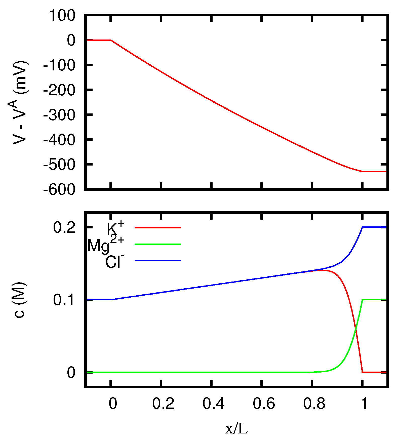
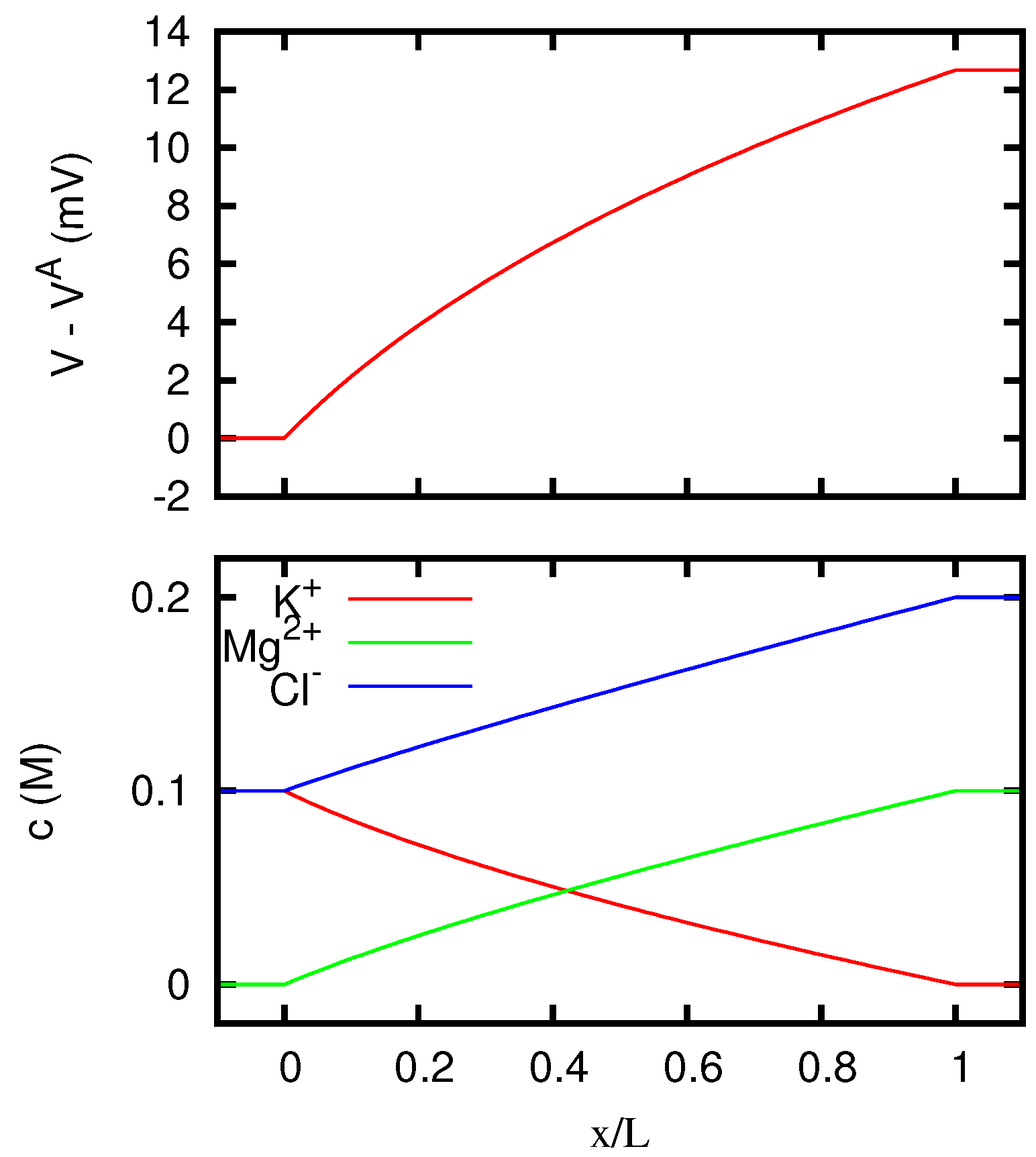
In Figure 1 we display the behavior of the electric potential and of the ionic concentrations inside the junction according to the Nernst–Planck equation. We see that for vanishing current the concentrations inside the junction are with good approximation linearly dependent on the position, and this explains why the discrepancy between Nernst–Planck’s and Henderson’s predictions for the junction potential is quite small.

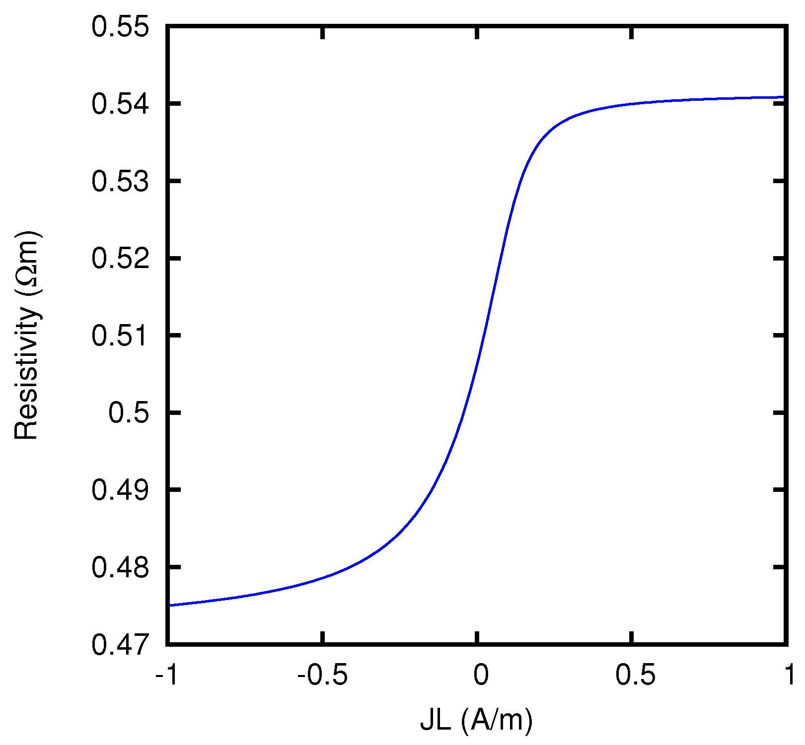
By using the formulas of Section 5.4, we can also calculate the junction potential as a function of the current flowing through the junction. If we then evaluate the effective resistivity of the junction according to Equation (40), we obtain the results which are displayed in Figure 2. We see that, when a large current flows from the KCl solution to the MgCl₂ solution, the Nernst–Planck resistivity is more than 10% larger than when a large current flows in the opposite direction.

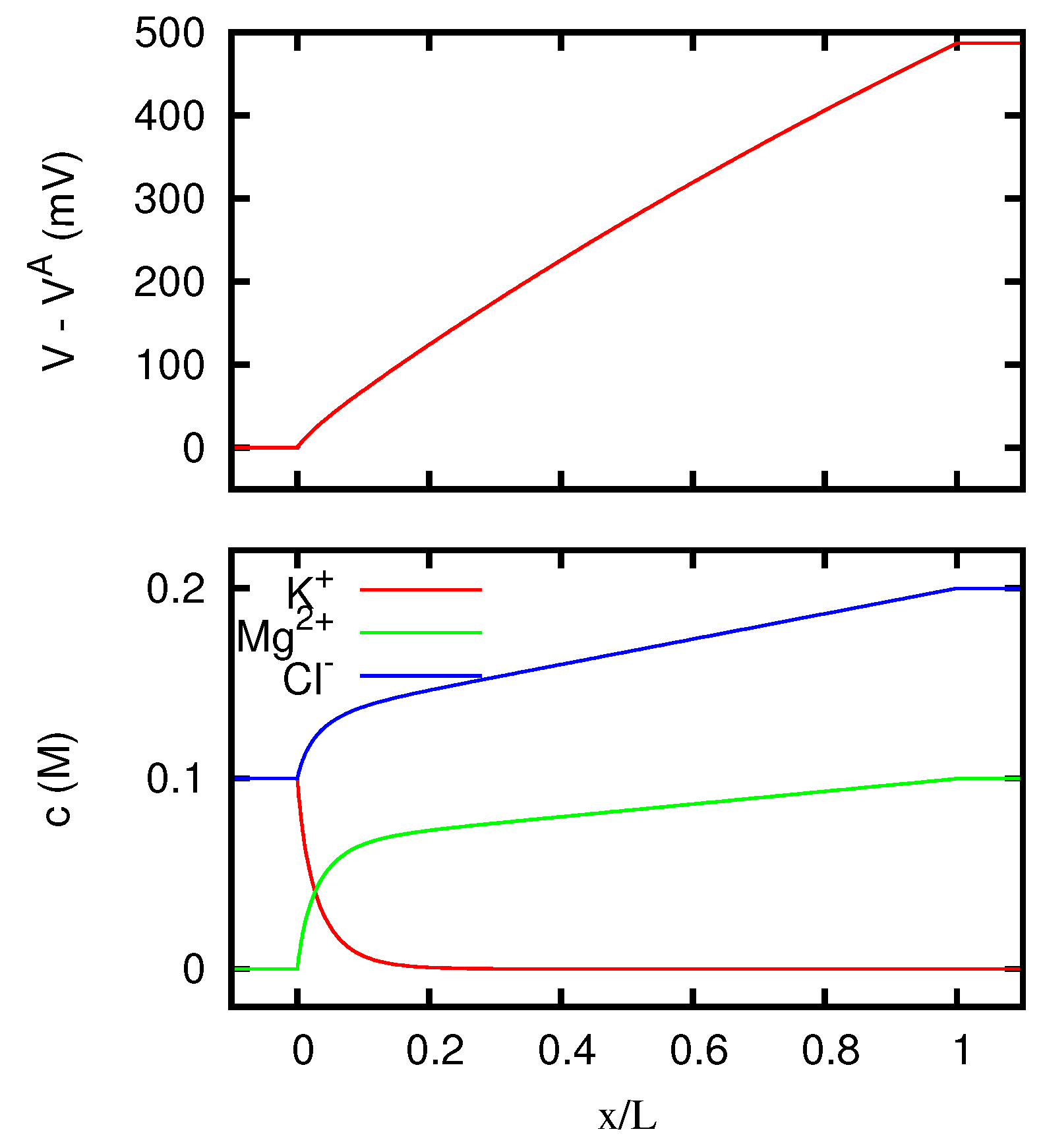
The behavior of the ionic concentrations inside the junction is displayed in Figure 3 for JL = 1 A/m, and in Figure 4 for JL = −1 A/m. We see that the results are in agreement with the conclusions of Section 5.3. Note in fact that a solution 0.1 M of MgCl₂ has the same w as a solution 0.15 M of KCl. For large positive current densities, the concentration profiles inside the junction are thus similar to the linear profiles of a junction between two KCl solutions 0.1 M and 0.15 M respectively. The effective resistivity of such a junction, according to Equation (53), is 0.5413 Ωm, and this is in fact the value that the curve of Figure 2 approaches for JL → +∞. In this limit, Mg²⁺ ions are present inside the junction only in a narrow region near to the right side. Similarly, since a solution 0.1 M of KCl has the same w as a solution 0.06667 M of MgCl₂, for large negative current densities the concentration profiles inside the junction tend to the linear profiles of a junction between two MgCl₂ solutions 0.06667 M and 0.1 M respectively. Such a junction has an effective resistivity of 0.4703 Ωm, which indeed corresponds to the limit of the curve of Figure 2 for JL → −∞. In this limit, K⁺ ions are present inside the junction only in a narrow region near to the left side.

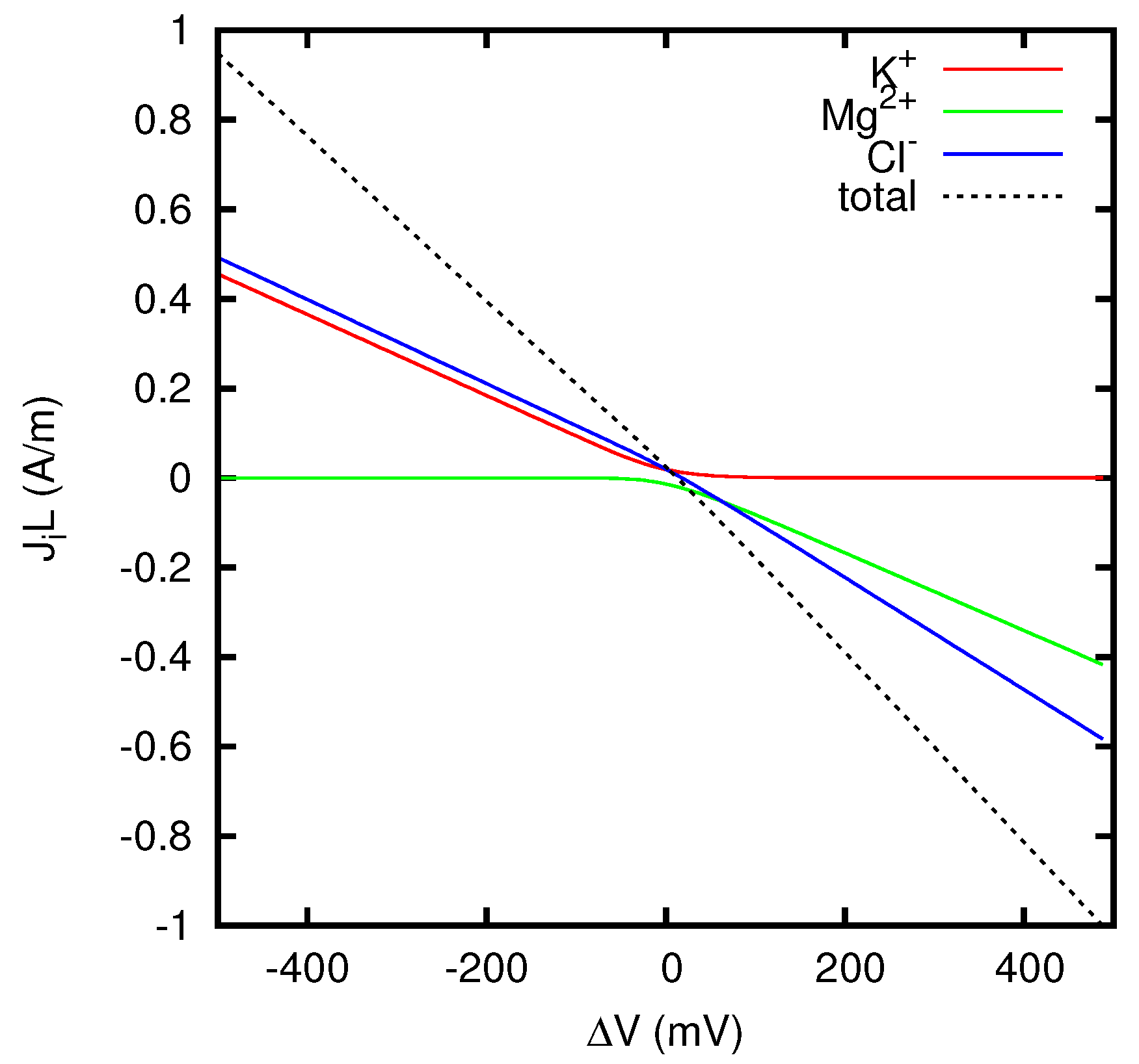
In Figure 5 we report the contributions to the quantity JL which come from the individual ion species. The contribution of the ion i is defined as $J_{i}L=e{z}_i{\Phi }_{i}L$, where ${\Phi }_i$ can be calculated using Equations (68)–(70). For JL = 1 A/m, the ratios $J_i/J$ between the partial currents of the ions and the total current are reported in the first column of

Table 1. Partial currents in a liquid junction between KCl 0.1 M and MgCl₂ 0.1 M, for JL = 1 A/m (column 2) and JL = −1 A/m (column 4), compared respectively with transference numbers in a KCl solution (column 3) and in a MgCl₂ solution (column 5).

Ion	JiL/(A/m)	ti (KCl)	−JiL/(A/m)	ti (MgCl2)
K+	0.481	0.491	−7 × 10−9	0
Mg2+	−1 × 10−18	0	0.418	0.410
Cl−	0.519	0.509	0.582	0.590

. These values are very close to the corresponding transference numbers in a KCl solution, as shown in the second column of Table 1. Similarly, for JL = −1 A/m, the ratios $J_i/J$ are very close to the corresponding transference numbers in a MgCl₂ solution (see third and fourth columns of Table 1). These results are clearly in agreement with Equations (84) and (88).

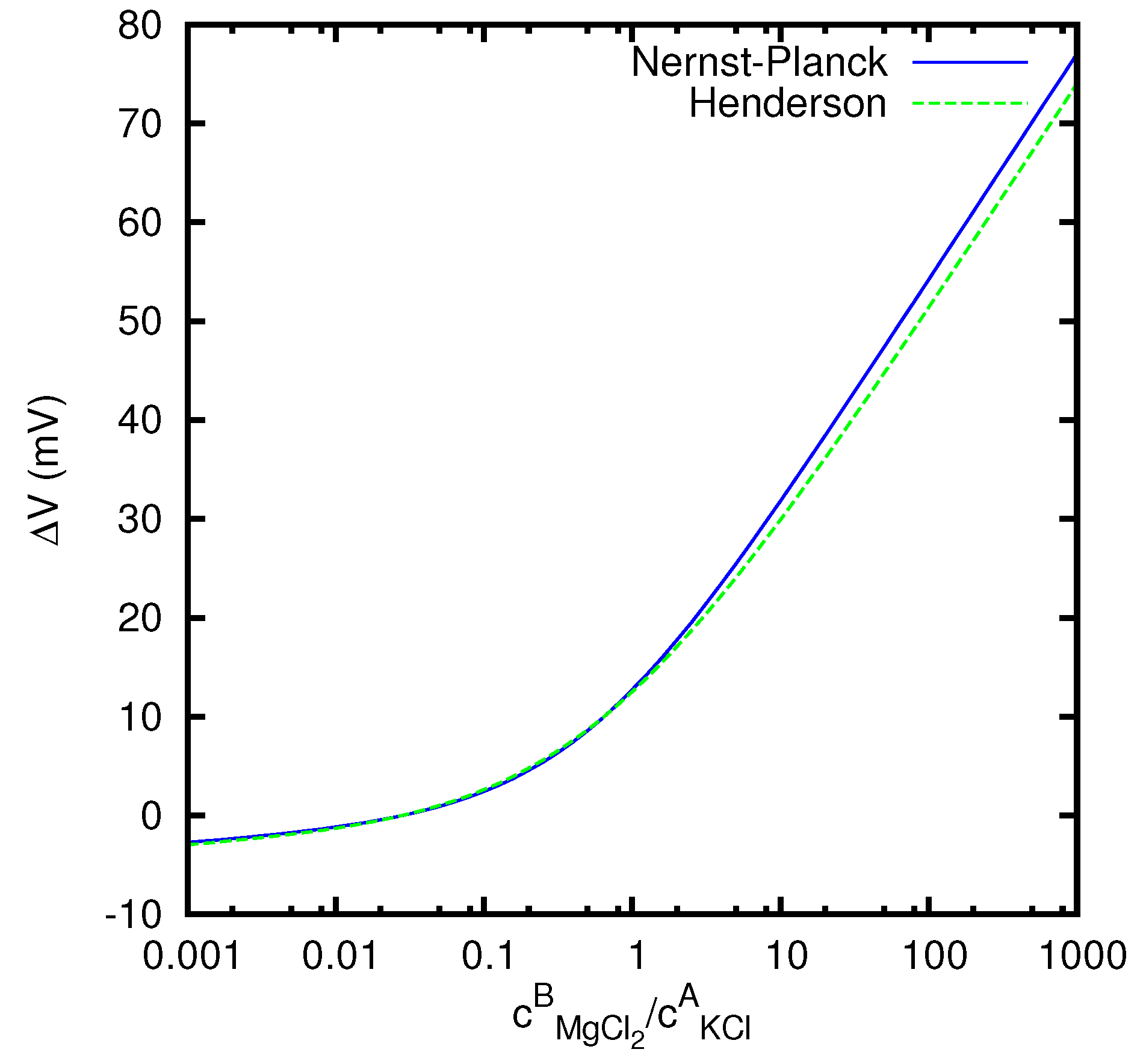
Finally, in Figure 6 we study the dependence of the junction potential, for vanishing current, on the ratio $c_{{\text{MgCl}}_2}^B/c_{\text{KCl}}^A$ between the concentrations of the MgCl₂ solution on the first side and of the KCl solution on the second side. We see that the absolute value of the junction potential is considerably higher when the concentration of the MgCl₂ solution prevails with respect to the concentration of the KCl solution. This is related to the fact that the mobility of the Mg²⁺ ion is about 65% lower than the mobility of the Cl⁻ ion, whereas the difference between the mobilities of K⁺ and Cl⁻ is less than 4%. This implies that MgCl₂ gives to the junction potential a stronger contribution than KCl.

7.3. Uphill Transport of Minority Ionic Species

In a system with at least three different ionic species, it is possible to observe in some cases the interesting phenomenon called “uphill transport”, in which one species is transported by the electric field, generated by the liquid junction at open circuit, against its concentration gradient. This effect has been well studied in perm-selective membranes [45,46] and is relevant for the reverse electrodialysis technique for the production of energy from salinity differences [47,48], since it generates an unwanted accumulation of magnesium ions from sea water that affects the performances of the device.

An application of our method to the theoretical prediction of this phenomenon for charged membranes will be presented in Section 7.4. The uphill transport can however be observed also in neutral liquid junctions, and Figure 7 shows the results of the calculations for two systems in which this phenomenon indeed takes place. We consider a liquid junction between two solutions of HCl, with concentration 10 mM at the side x = 0 (solution A) and 100 mM at the side x = L (solution B), at T = 298.15 K. Solutions with Hydrogen ions are considered in this example, since their high mobility (we have D = 9.311 × 10⁻⁹ m² s⁻¹ for the diffusion coefficient of H⁺ at 25 °C [44]) enhances the phenomenon which we want to study (see [18] for the investigation of a similar situation in charged membranes). We suppose that the two solutions also contain a second electrolyte, namely the chloride of a different cation, with much smaller concentrations which we shall call $c_{\text{min}}^A$ and $c_{\text{min}}^B$, since they correspond to the concentrations of the minority cation in the two solutions A and B. We fix $c_{\text{min}}^A=0.1$ mM at x = 0, and we study the flux of the minority cation as a function of the concentration $c_{\text{min}}^B$ at x = L (roughly speaking, as a function of the concentration gradient), at zero total current. We shall consider two situations: in the first one the minority electrolyte in the two solutions is KCl, and so we have in the junction a univalent minority cation K⁺; in the second one the electrolyte is instead MgCl₂, and so we have a divalent minority cation Mg²⁺.

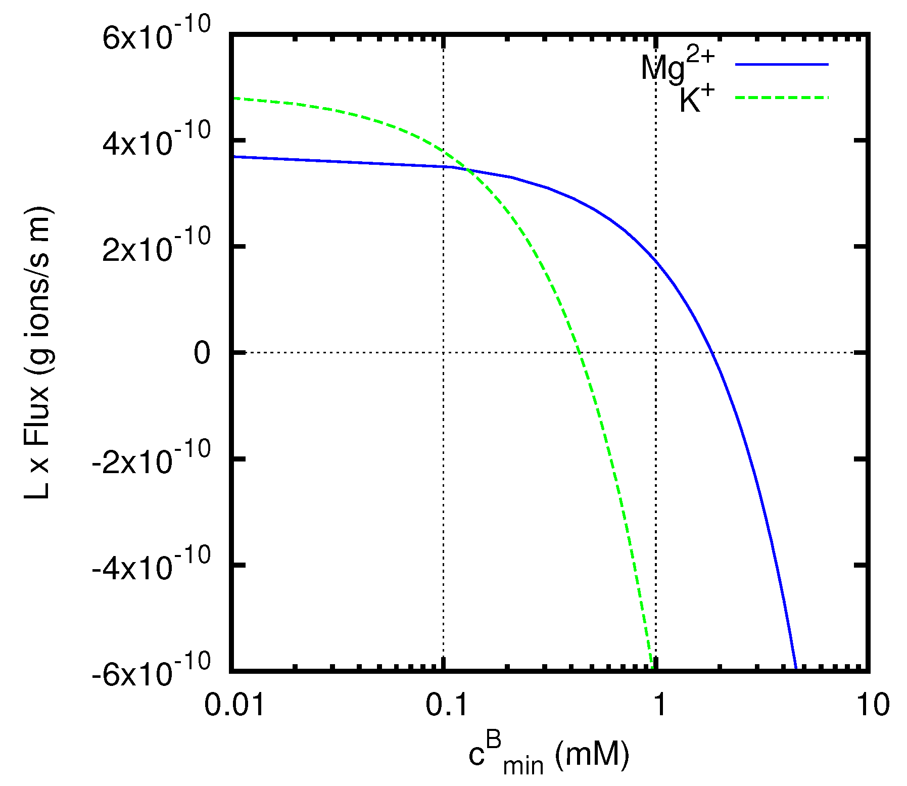
The graph in Figure 7 reports the fluxes of the minority cations (multiplied by the thickness L of the junction) calculated by means of Equation (69). The positive direction of the fluxes corresponds to that of the x-axis, and so goes from solution A to solution B. In the region of the graph for $c_{\text{min}}^B>0.1$ mM the diffusive Fick’s flux for the minority cation would be negative. Nevertheless, we observe positive values of the actual flux in a considerable range of concentrations above that value, especially for Mg²⁺ ions, representing an uphill transport of the ion, i.e., a transport against the diffusive Fick’s flow.

The fluxes of the majority ions H⁺ and Cl⁻ are weakly affected by the presence of the minority electrolyte, and are not shown in the figure. We have from Equations (68) and (70) ${\Phi }_{{\mathrm{H}}^{+}}L\approx {\Phi }_{{\mathrm{Cl}}^{-}}L\approx -3\times {10}^{-7}$ g ions/s m. A liquid junction potential of approximately −38 mV, essentially independent of the minority electrolyte, develops across the liquid junction, due to the fact that the mobility of H⁺ ions is significantly larger than that of Cl⁻ ions. This potential generates an electric field directed along the positive x axis.

At values of $c_{\text{min}}^B$ less than the concentration $c_{\text{min}}^A=0.1$ mM of the minority cation at x = 0, both the diffusive Fick’s flux and the flux induced by the electric field are positive. At values of $c_{\text{min}}^B$ approaching the concentration at x = 0, i.e., $c_{\text{min}}^A\approx c_{\text{min}}^B$, the concentration gradient, and thus the diffusive Fick’s flux, vanish. In this situation, the minority cations (Mg²⁺ or K⁺) will be dragged by the electric field generated by the liquid junction and will generate a flux with positive sign, i.e., directed as the positive x-axis. The same will be true in the presence of an opposing concentration gradient, provided that the diffusive Fick’s flux it generates is small compared to the flux induced by the electric field. This phenomenon is responsible for the uphill transport observed for both K⁺ and Mg²⁺ ions at concentrations $c_{\text{min}}^B\gtrsim c_{\text{min}}^A$.

At higher values of $c_{\text{min}}^B$, the behaviors of K⁺ and Mg²⁺ ions become remarkably different from one another. A particularly significant value of concentration is $c_{\text{min}}^B=1$ mM, at which the ratio between the concentration of the minority electrolyte and that of HCl takes the same value (namely 1/100) at the two sides of the junction. At this concentration, the system can be formally treated as containing a single electrolyte with three different ion species, and the concentrations of all the ions have fixed ratios along the liquid junction. This implies that all the cations with the same charge will have the same flux direction. In particular, both H⁺ and K⁺ ions will be transported towards the less concentrated region, giving the negative flux observed for the K⁺ ion at $c_{\text{min}}^B=1$ mM, which corresponds to the usual downhill transport. Instead, due to its higher charge, the Mg²⁺ ions still show an uphill transport, that also persists at even higher values of opposing concentration gradients.

For both K⁺ and Mg²⁺ ions, when the concentration gradient becomes strong enough, the diffusive Fick’s flux finally overcomes the uphill transport generated by the liquid junction potential, and thus negative values of the flux are observed for sufficiently high values of $c_{\text{min}}^B$.

It is worth noting that, when the ratio between the concentrations of the two electrolytes is the same at the two sides of the junction (i.e., for $c_{\text{min}}^B=1$ mM in the example considered above), the assumptions at the basis of Henderson’s method become verified, and the values of the fluxes resulting from the Nernst–Planck equations can be computed by rather elementary means. However, for arbitrary concentrations Henderson’s method does not provide results comparable with those reported in Figure 7, since in general it does not allow definite predictions for the fluxes of the individual ion species. Note also that the most interesting situation for the uphill transport, i.e., that with both univalent (H⁺) and divalent (Mg²⁺) ions present together, cannot be treated with Planck’s method of solution, and so can be solved analytically only with more advanced procedures as those presented in this paper.

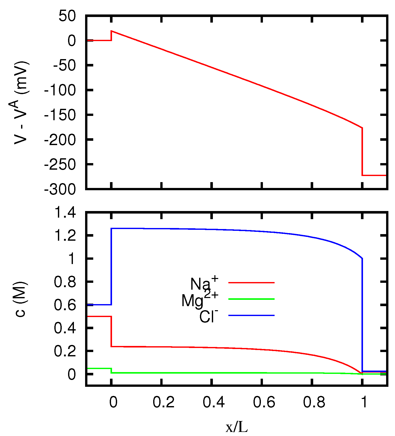
7.4. Charged Membranes between Solutions of NaCl and MgCl₂

As an example of application of our methods to the study of charged membranes, let us consider a membrane between solutions of a mixture of two salts, with identical ratios with respect to one another at the two sides of the membrane, but with concentrations which are considerably higher at one side than at the other. In particular, we shall consider a solution NaCl 0.5 M, MgCl₂ 50 mM at the first side, and a solution NaCl 20 mM, MgCl₂ 2 mM at the second side. Thus in this section indexes 1, 2, and 3 will refer to ions Na⁺, Mg²⁺, and Cl⁻ respectively, and we will use the diffusion coefficients D₁ = 1.334 × 10⁻⁹ m² s⁻¹, D₂ = 0.706 × 10⁻⁹ m² s⁻¹, D₃ = 2.032 × 10⁻⁹ m² s⁻¹ [44], at T = 298.15 K. We also assume ${\eta }_1={\eta }_2={\eta }_3=1$ and, in Equations (7) and (8), $k_1=k_2=k_3=1$.

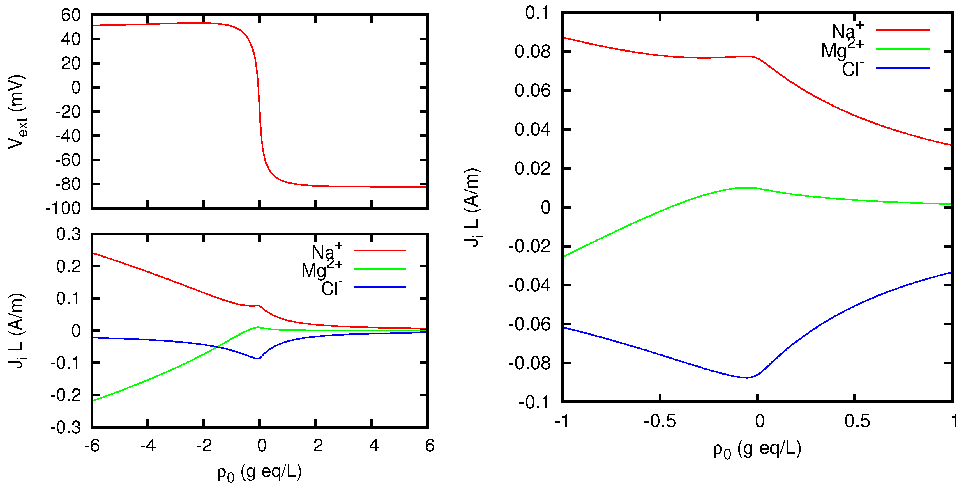
In Figure 8 we show the potential difference between the two solutions, and the current carried by each ionic species, for vanishing total current, as functions of the density of fixed charges in the membrane, represented as in Equation (3) by the quantity ${\rho }_0$ (${\rho }_0=1$ g eq/L corresponds to a charge density of 96,485 C/L). It can be noticed that for ${\rho }_0\to +\infty$ the membrane potential tends to the Donnan limit $V_D^{+}=-(kT/e)log(c_3^A/c_3^B)=-82.70$ mV. For ${\rho }_0\to -\infty$ the Donnan potential is mainly determined by the divalent cation, and the limiting value of the membrane potential is $V_D^{-}=(kT/2e)log(c_2^A/c_2^B)=41.35$ mV. However, the presence also of univalent ions affects the behavior of the membrane in such a way that a maximum potential of 53.24 mV is reached for a finite value of the background charge density, namely ${\rho }_0\approx -2.20$ g eq/L. A remarkable fact is that local maxima of all the ion fluxes are reached for ${\rho }_0\approx -0.06$ g eq/L. One can also notice that for ${\rho }_0<-0.45$ g eq/L the flux of Mg²⁺ ions becomes negative, which corresponds to the well-known phenomenon of the uphill transport of minority ions, already discussed in the preceding section.

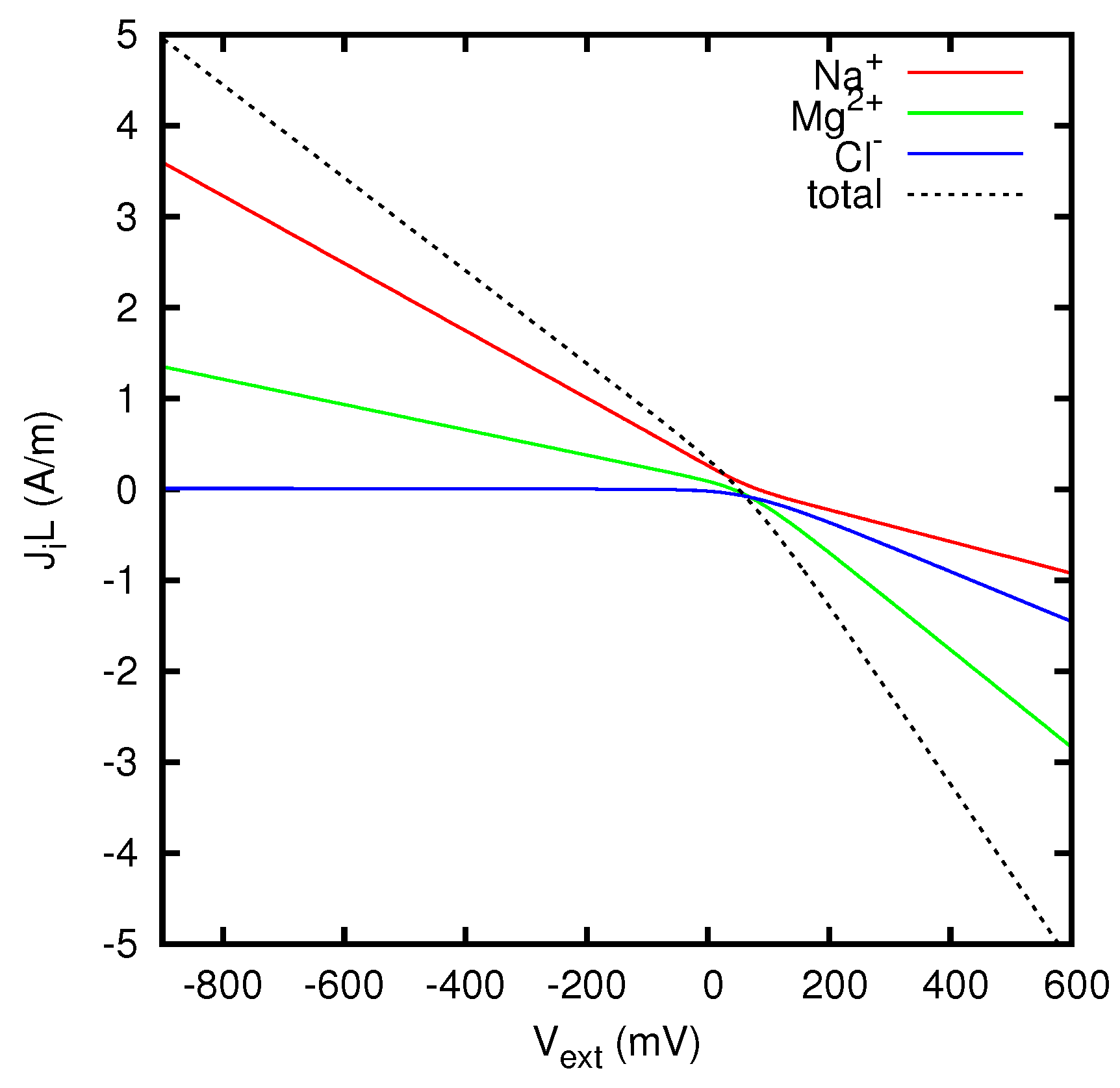
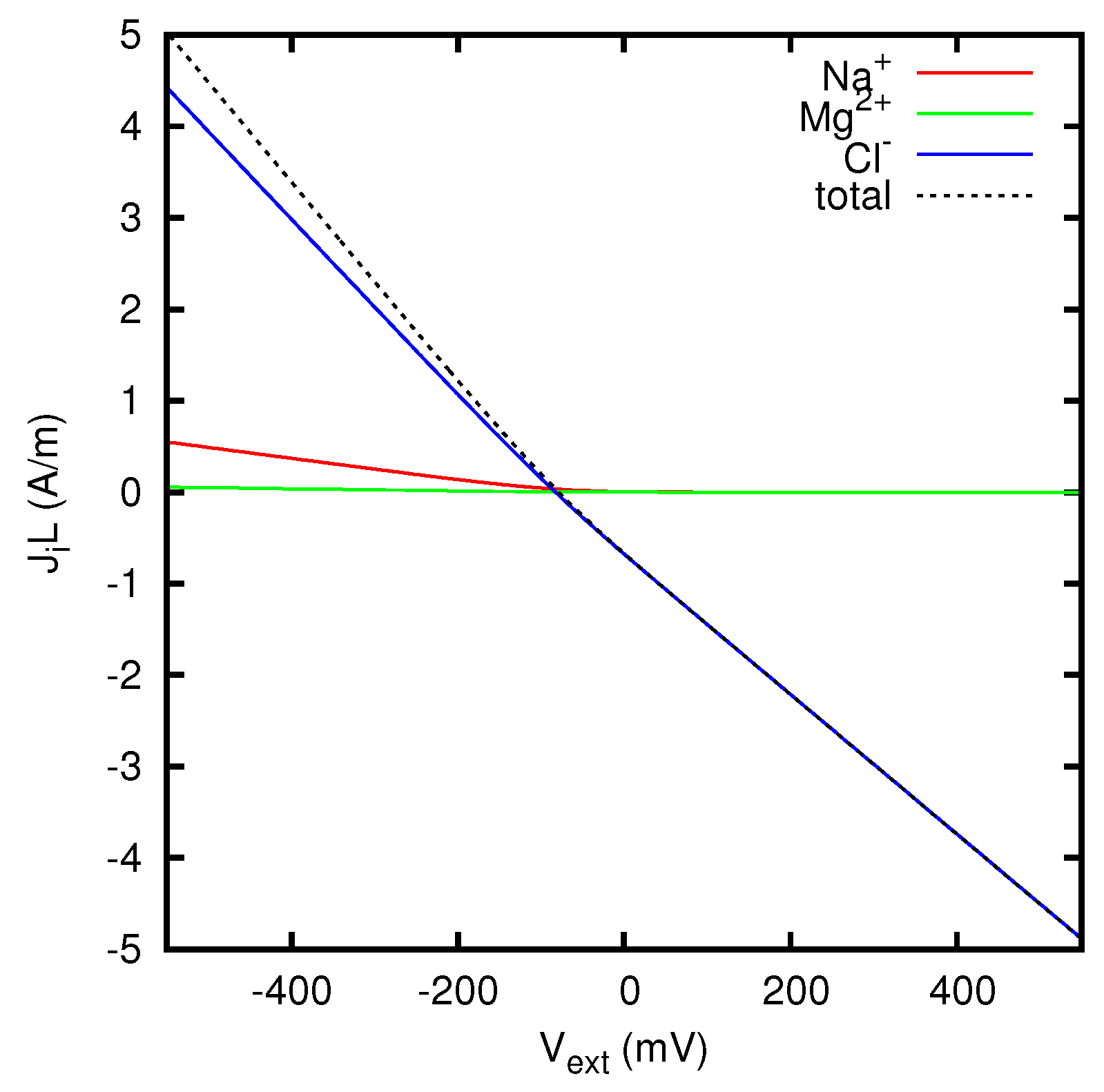
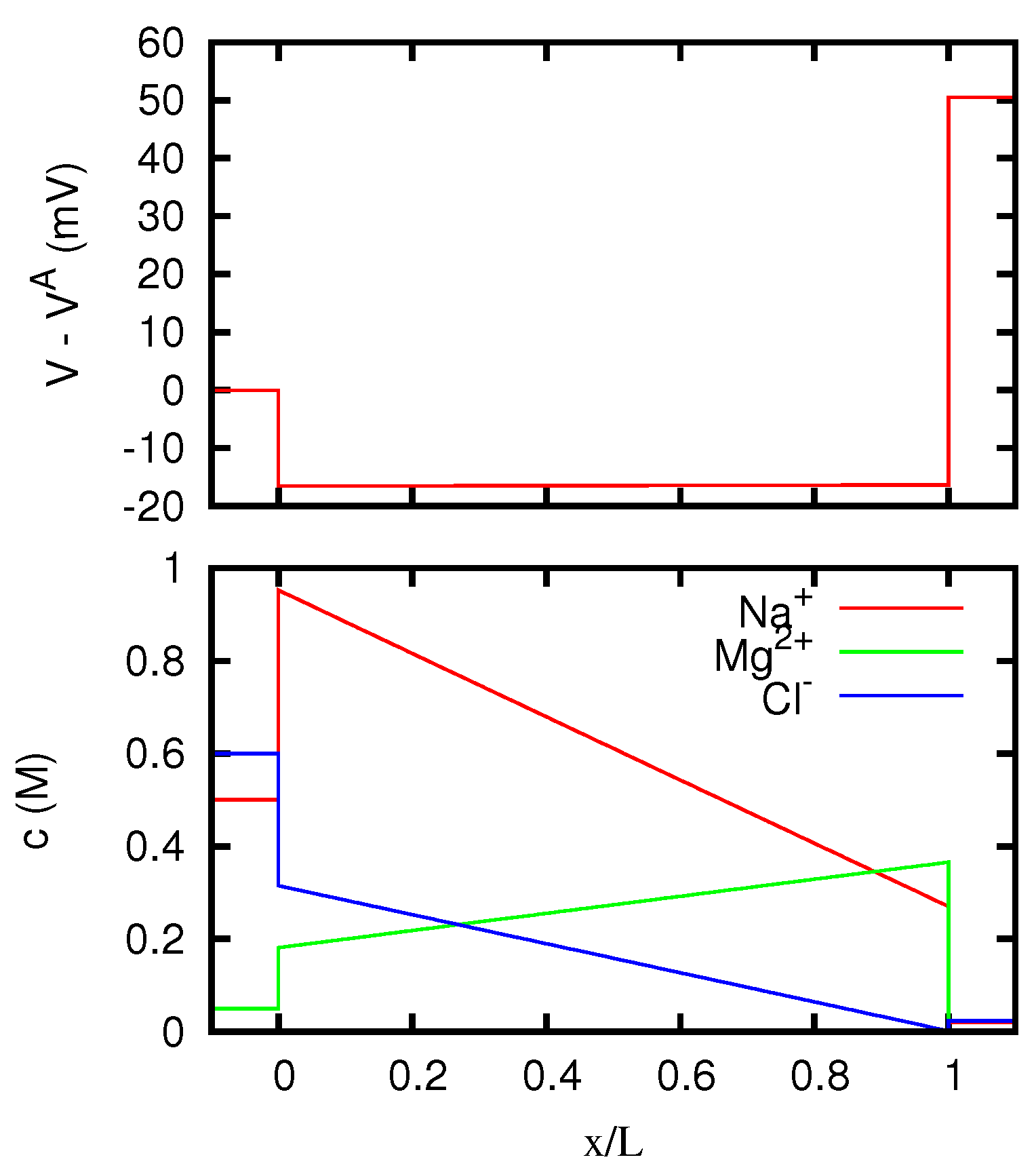
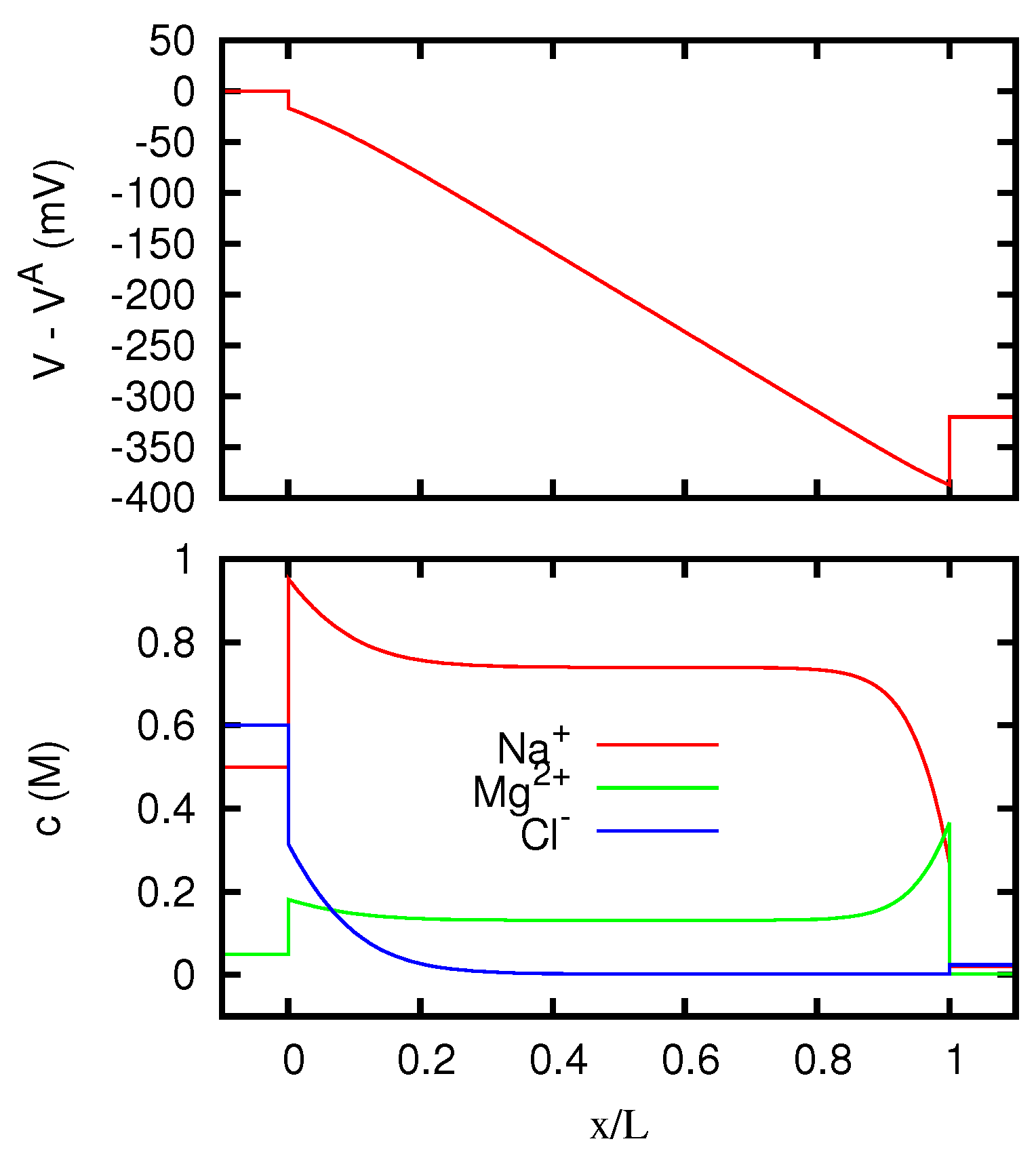
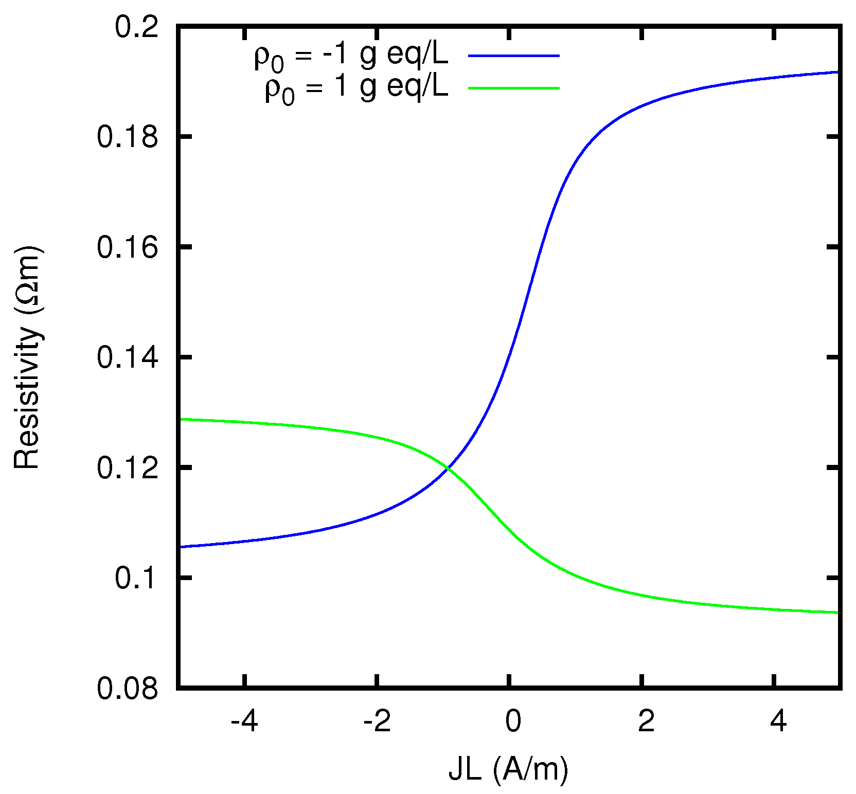
In Figure 9 we display the ionic currents as functions of the potential difference between the two solutions, for an AEM (anion exchange membrane) with a density of positive fixed charges such that ${\rho }_0=1$ g eq/L. A similar study is presented in Figure 10 for a CEM (cation exchange membrane) with ${\rho }_0=-1$ g eq/L. The resulting behavior of the effective resistivity of the junction as a function of the current is shown in Figure 11. 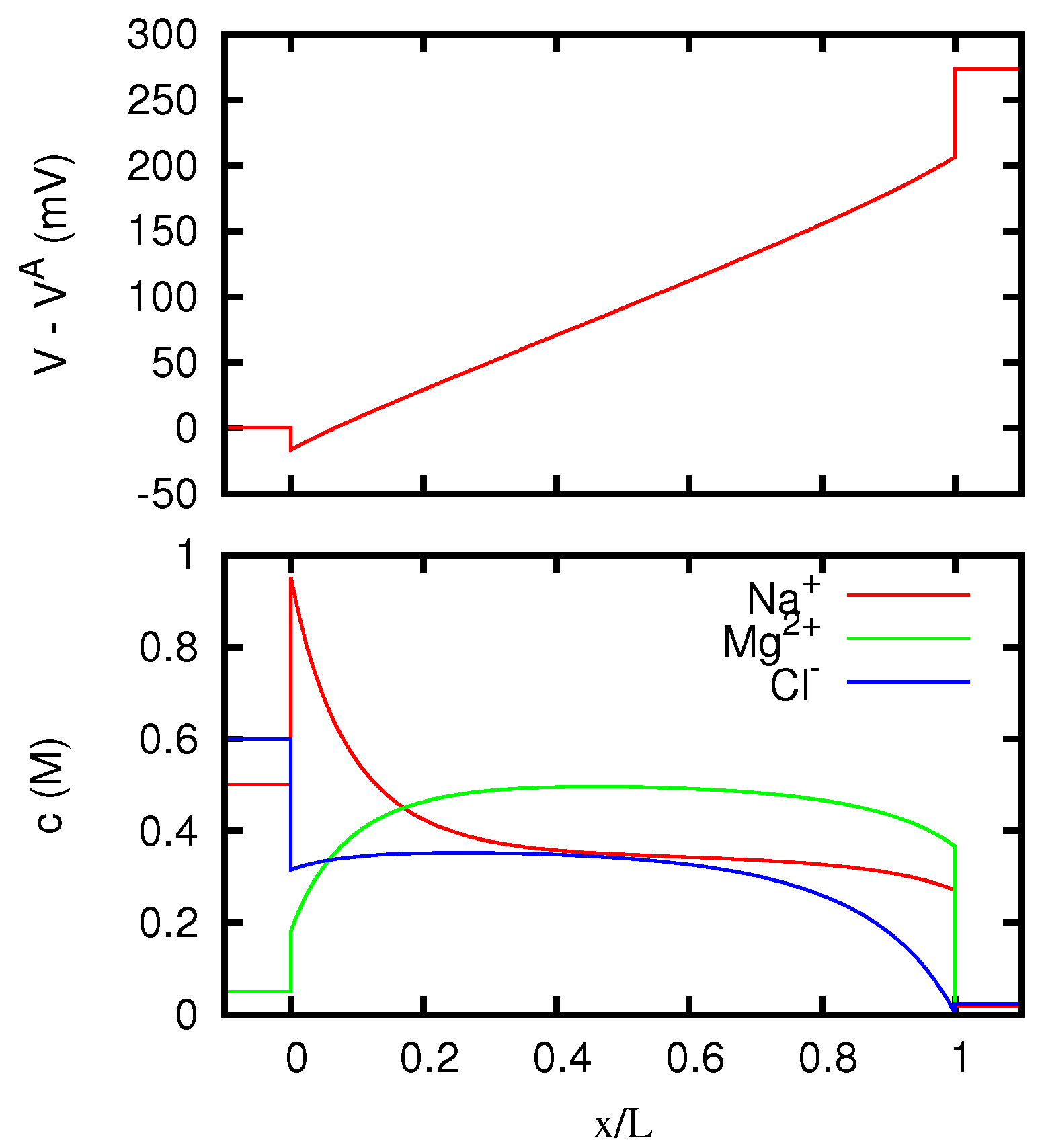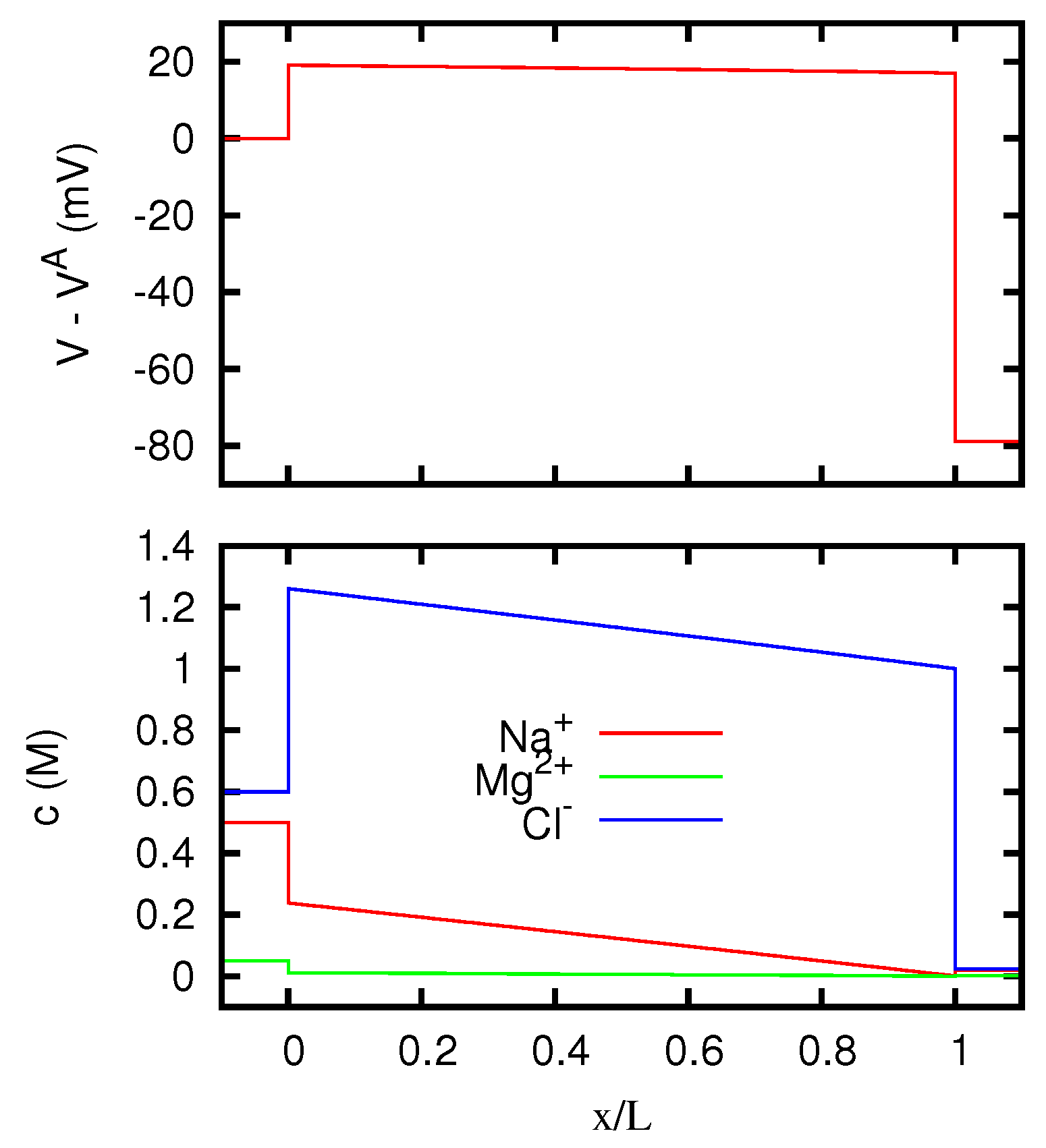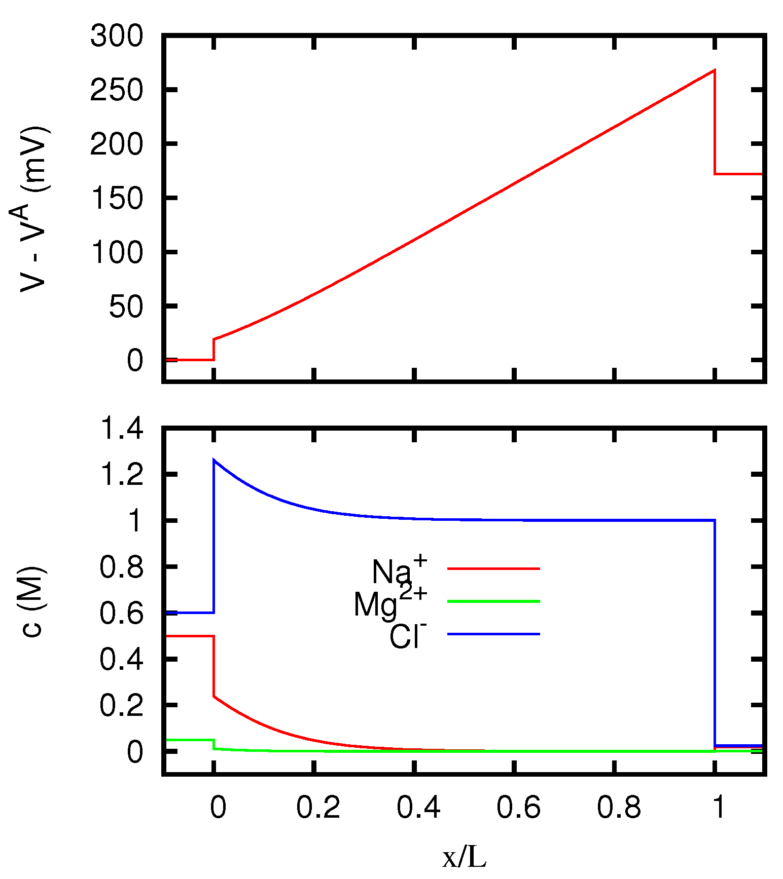The difference between the limiting values of the resistivity at the two sides of the graph is due to the dependence of the ionic concentrations on the current, as mathematically discussed in Section 5. Such a dependence is illustrated for the AEM in Figure 12, Figure 13 and Figure 14, and for the CEM in Figure 15, Figure 16 and Figure 17, by considering the potential and concentration profiles inside the junction for particular values of the current. One can observe that the results are in agreement with the general analysis of Section 5.2. In particular, in the case of the AEM (for which only one counterion is present) the ion concentrations inside the membrane approach for high currents the values at the boundary from which the coions Na⁺ and Mg²⁺ enter the membrane. According to Equations (78) and (79), the curve for ${\rho }_0=1$ g eq/L of Figure 11 tends to the limits 0.1309 Ωm for $JL\to -\infty$ and 0.0915 Ωm for $JL\to +\infty$. The limits of the curve for ${\rho }_0=-1$ g eq/L are instead 0.1014 Ωm for $JL\to -\infty$ and 0.1959 Ωm for $JL\to +\infty$. So the limiting resistivity of the CEM between the two solutions considered is in one of the two directions almost twice as big as in the other.

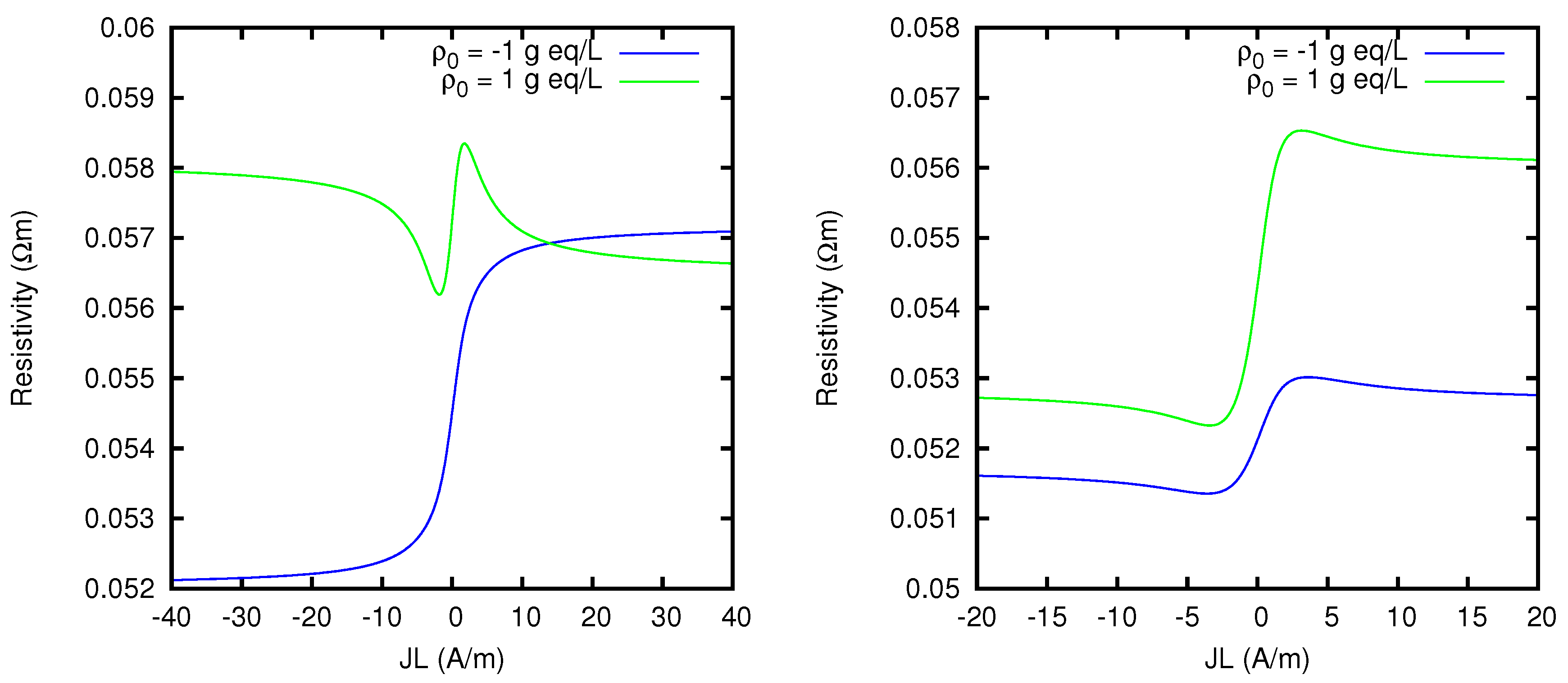
The Nernst–Planck model is able to reveal detailed features of the behavior of a charged membrane which, although not necessarily relevant from a quantitative point of view, are nevertheless qualitatively quite remarkable. As an example, we show in Figure 18 the effective resistivity of charged membranes between solutions of mixtures of NaCl and MgCl₂, with different concentrations from those previously considered. We see that small variations in the composition of the two solutions affect in a significant way the behavior of the resistivity, which can present minima and maxima as a function of the current density flowing through the membrane.

8. Conclusions

In the present paper we have solved the Nernst–Planck equations for an ideal constrained liquid junction or charged membrane, and we have provided analytical expressions for the junction potential, the resistivity and the ionic fluxes, as well as for the potential and concentration profiles inside the diffusion layer. These analytical expressions have been given for an arbitrary value of the total current density flowing through the junction or membrane, and are valid for systems containing up to three different ionic species with arbitrary valence. We have also shown that the results can be generalized with not too much difficulty to the case of an arbitrary number of ionic species, provided that the total number of valences is not greater than three.

Although the problem considered in this paper has already been the subject of several investigations, the form of our analytical results is new, and they can be rather easily applied to obtain quantitative predictions in a wide range of practical situations. The only step which needs to be performed with a computer is as simple as locating the zero of a function of one real variable. Using these methods it is thus possible to obtain in a simple and reliable way a set of results which are usually derived by means of heavy ad hoc numerical routines. Therefore our results may represent a useful tool for researchers having to study problems involving the behavior or either charged or uncharged liquid junctions in not too complex chemical systems.

We have applied our procedure to the study of a few concrete situations. Our results confirm that the simple Henderson model generally agrees with the predictions of the Nernst–Planck model, as far as the value of the junction potential at zero current is concerned. Nevertheless, the Nernst–Planck model provides a much more general and complete description of the system, including the ionic fluxes and distributions for arbitrary values of the total electric current flowing through the junction. As a result, it is able to highlight interesting features of the behavior of a system, that disappear in the rougher description given by Henderson’s model. A remarkable example is given by the uphill transport of a divalent ion, i.e. its global flow from the side with lower concentration to the side with higher concentration of a liquid junction or of a charged membrane, which may occur at open circuit in the presence of a majority of univalent ions with the same sign.