An Incompressible, Depth-Averaged Lattice Boltzmann Method for Liquid Flow in Microfluidic Devices with Variable Aperture

Abstract

Two-dimensional (2D) pore-scale models have successfully simulated microfluidic experiments of aqueous-phase flow with mixing-controlled reactions in devices with small aperture. A standard 2D model is not generally appropriate when the presence of mineral precipitate or biomass creates complex and irregular three-dimensional (3D) pore geometries. We modify the 2D lattice Boltzmann method (LBM) to incorporate viscous drag from the top and bottom microfluidic device (micromodel) surfaces, typically excluded in a 2D model. Viscous drag from these surfaces can be approximated by uniformly scaling a steady-state 2D velocity field at low Reynolds number. We demonstrate increased accuracy by approximating the viscous drag with an analytically-derived body force which assumes a local parabolic velocity profile across the micromodel depth. Accuracy of the generated 2D velocity field and simulation permeability have not been evaluated in geometries with variable aperture. We obtain permeabilities within approximately 10% error and accurate streamlines from the proposed 2D method relative to results obtained from 3D simulations. In addition, the proposed method requires a CPU run time approximately 40 times less than a standard 3D method, representing a significant computational benefit for permeability calculations.

1. Introduction

Understanding reactive flow and transport processes at the pore scale has benefited from model validation against experimental results using microfluidic devices. Also referred to as micromodels, these devices serve as model porous media in laboratory experiments studying pore-scale reactive transport processes [1,2] (see Figure 1). Micromodel experiments of solute mixing and reaction [3], calcium carbonate (CaCO${}_3$) precipitation [4], and biomass growth [5,6] have been numerically modeled by solving the Stokes equations for the flow field followed by the advection-diffusion-reaction equations for concentration fields.

Due to the need to simulate small cross-sectional aspect ratios, i.e., the ratio of flow aperture to width, some numerical models approximate the micromodel as a 2D system [3,4,5,6,7]. For special cases where the micromodel aperture is constant, 2D numerical models appear to accurately capture flow, transport, and reaction [3,7]. Such models are computationally efficient and avert costly 3D numerical methods. However, when micromodel aperture is variable due to reactions that promote biomass or mineral precipitate growth on its top and bottom surfaces, 2D flow models are not expected to accurately capture the complex 3D flow paths that develop.

Figure 1. (a) Entire micromodel with a regular pore network of cylindrical pillars; (b) Perspective view of micromodel interior taken with scanning electron microscope. Pillars span the entire aperture; (c) Close-up side view of micromodel with CaCO${}_3$ on top (glass) and bottom (silicon) surfaces. Precipitate appears in gray against a black background of empty pore space. Image taken with environmental scanning electron microscope (Philips/FEI XL30 ESEM-FEG, Urbana, IL, USA); (d) Streamwise slice of randomly-generated symmetric aperture, denoted $h(x,y)$, between cylindrical pillars. White and black colors represent liquid and solid phases, respectively.

Figure 1. (a) Entire micromodel with a regular pore network of cylindrical pillars; (b) Perspective view of micromodel interior taken with scanning electron microscope. Pillars span the entire aperture; (c) Close-up side view of micromodel with CaCO${}_3$ on top (glass) and bottom (silicon) surfaces. Precipitate appears in gray against a black background of empty pore space. Image taken with environmental scanning electron microscope (Philips/FEI XL30 ESEM-FEG, Urbana, IL, USA); (d) Streamwise slice of randomly-generated symmetric aperture, denoted $h(x,y)$, between cylindrical pillars. White and black colors represent liquid and solid phases, respectively.

Some numerical models indirectly account for the micromodel aperture. For example, the CaCO${}_3$ precipitation model of Yoon et al. [4] assumes precipitate grows exclusively on the top and bottom micromodel surfaces, motivated by the experimental observation depicted in Figure 1c. These surfaces are outside the horizontal plane of a 2D simulation, and there is no accounting for the impact of precipitate on flow. If instead a fully 3D model were used, a very fine grid would be required where the aperture was highly constricted. In this work, we propose a modified 2D flow model rather than full 3D simulation, in order to maintain computational efficiency. The model is applicable to geometries in which one spatial dimension is very small relative to the others. Motivated by our previous work [1,3,4,6], we describe its application in microfluidics. More generally, it could approximate flow through rough-walled fractures and in bounded thin films.

We consider two ways in which the 2D velocity field can be affected by the restricted vertical dimension. First, the top and bottom surfaces, composed of glass, silicon, or reaction product, are no-slip boundaries that impart viscous drag on the liquid. This effect has been approximated in a 2D flow model for a micromodel with uniform aperture [8,9], but the approximation has not been evaluated in geometries of variable aperture with respect to accuracy of the velocity field and computed permeability. Second, spatial variation in aperture affects local velocity direction. For example, flow is diverted away from more constricted regions. The objective of this work is to incorporate a spatially-variable aperture in a depth-averaged 2D lattice Boltzmann model with viscous drag, determine if the approach yields improved results relative to a standard 2D flow model, and quantify its computational benefit relative to a fully 3D flow model. The proposed flow model is benchmarked in a micromodel unit cell and a heterogeneous pore geometry. Extending the approach to 2D and 3D models of solute transport and reaction is an important future research step, but outside the scope of this work.

In all test cases, 2D velocity fields are compared to the depth-averaged velocity field from a 3D lattice Boltzmann model, which we consider the true velocity field. We also compare the permeability estimated by the proposed 2D method with the true permeability computed by the 3D model, as lattice Boltzmann models are commonly used to compute the permeability of porous media [9,10].

2. Methods

2.1. Governing Equations

The lattice Boltzmann method (LBM) has been used in a number of fundamental investigations [11,12], including simulating Stokes flow in porous media [13,14]. Three-dimensional steady flow at low Reynolds number is governed by the incompressible continuity and momentum equations:

$$\begin{array}{cc}\hfill \nabla ·u_{3D}& =0\hfill \end{array}$$

(1)

$$\begin{array}{cc}\hfill \nu {\nabla }^2{u}_{3D}& =-a\hfill \end{array}$$

(2)

In which kinematic viscosity is ν, a is an external acceleration, and the 3D velocity vector $u_{3D}(x,y,z)={\left[u_{3D},v_{3D},w_{3D}\right]}^T$. Note all equations utilize common notation, where plain and bold font denote scalar and vector quantities, respectively. The forcing term on the right-hand side (RHS) of Equation (2) often accounts for the effect of gravitational acceleration. In this application, that term is a driving force representing the constant flow pumps used in micromodel experiments, where $a={\left[a_x,0,0\right]}^T$.

The 2D governing equations are derived in three steps. First, we depth-average Equations (1) and (2). Second, we assume the horizontal velocity components $u_{3D}(x,y,z)$ and $v_{3D}(x,y,z)$ have parabolic velocity profiles across the aperture $h(x,y)$, a familiar result from the literature in lubrication theory [15,16], making it possible to evaluate derivatives and integrals with respect to the vertical (z) coordinate. Third, we assume the vertical velocity component $w_{3D}(x,y,z)\approx 0$, a common assumption in fracture-like geometries [17], thereby eliminating the momentum equation in the vertical direction. The resulting equations are:

$$\begin{array}{cc}\hfill \nabla ·\left(u_{2D}h\right)& =0\hfill \end{array}$$

(3)

$$\begin{array}{cc}\hfill \nu {\nabla }^2\left(u_{2D}h\right)& =-\left[ha-{\displaystyle \frac{12\nu }{h^2}}\left(u_{2D}h\right)\right]\hfill \end{array}$$

(4)

where $h=h(x,y)$, $a={\left[a_x,0\right]}^T$, and $u_{2D}(x,y)={[u_{2D},v_{2D}]}^T$. Viscous drag from the top and bottom surfaces is approximated by the second forcing term on the RHS of Equation (4). Referred to as the viscous drag term, it was originally derived [18] for Hele-Shaw flow, i.e., flow between narrowly-spaced parallel surfaces, but has been applied successfully to micromodels with spatially-uniform aperture [8,9]. We extend use of the viscous drag term to cases of spatially-variable aperture.

Several flow models for micromodel experiments have omitted the viscous drag term and scaled the steady-state velocity field to match experimental Darcy velocity. This procedure is summarized by $cu(x,y)\to u(x,y)$, where c is a constant. To determine if uniform scaling alone can yield results equivalent to those using the viscous drag term, we perform 2D simulations, omitting that term, governed by:

$$\begin{array}{cc}\hfill \nabla ·\left(u_{2D}^{*}h\right)& =0\hfill \end{array}$$

(5)

$$\begin{array}{cc}\hfill \nu {\nabla }^2\left(u_{2D}^{*}h\right)& =-ha\hfill \end{array}$$

(6)

where $u_{2D}^{*}(x,y)={\left[u_{2D}^{*},v_{2D}^{*}\right]}^T$. A major aim of this work is to evaluate the accuracy of $u_{2D}^{*}(x,y)$ and $u_{2D}(x,y)$ in geometries with spatially-variable aperture.

It should be noted that $u_{2D}^{*}(x,y)$ and $u_{2D}(x,y)$ are uniformly scaled to ensure their flow rate is equivalent to that of the true velocity field prior to comparison. The only difference between these 2D velocity fields is whether or not they were generated under the influence of the viscous drag term. No scaling is performed for the purpose of computing permeability, as that would artifically produce a perfect result.

2.2. The Lattice Boltzmann Method: A Brief Overview

The LBM is an explicit in time solver of the Navier-Stokes equations. The fluid is represented by a set of pseudo-particles, whose motion is represented via probability distribution functions (PDFs), propagate and collide on a lattice [19]. Spatial and temporal evolution of PDFs is governed by the lattice Boltzmann equation:

$$f_i\left(x+e_i\Delta t,t+\Delta t\right)=f_i\left(x,t\right)+\Omega \left[f_i\left(x,t\right)\right]+\Delta t{F}_i$$

(7)

where $f_i$ denotes the PDF in the ith lattice direction defined by $e_i$, the position of a lattice node is x, t is the current time, $\Delta t$ the time step, Ω the collision operator, and $F_i$ a body force in the ith lattice direction. The equations presented in this section apply in general for both 2D and 3D lattice Boltzmann methods. Any differences in implementation, aside from the dimension of vector quantities, will be detailed in later sections. Ω is often represented by the Bhatnagar-Gross-Krook (BGK) operator [20]:

$$\Omega \left[f_i\left(x,t\right)\right]=-{\displaystyle \frac{1}{\tau }}\left[f_i\left(x,t\right)-f_i^{eq}\left(\rho ,u\right)\right]$$

(8)

in which particle collision is modeled as a relaxation toward local Maxwellian equilibrium, $f_i^{eq}(\rho ,u)$, with a single relaxation time, τ, which we set to 1.1 in all simulations. We acknowledge that multiple relaxation time methods [21] (Chapter 1) are preferable for their greater numerical stability [22,23] and because they do not suffer from viscosity-dependence of the computed permeability [13]. Because our aim is to match permeabilities from 2D and 3D models with equivalent viscosity, we select the single relaxation time method for its simplicity.

Continuum-scale equations can be derived from Equation (7), with the BGK operator, via Chapman-Enskog expansion [19] (Chapter 1). These equations differ from the Navier-Stokes equations by additional terms that introduce weak compressibility [19] (Chapter 6). An incompressible LBM [24] has been developed, which reduces the compressibility artifact by several orders of magnitude. All references to the LBM in this work imply use of this incompressible formulation. The equilibrium distribution function (EDF) is defined by:

$$f_i^{eq}\left(\rho ,u\right)=w_i\left[\rho +3(e_i·u)+{\displaystyle \frac{9}{2}}{(e_i·u)}^2-{\displaystyle \frac{3}{2}}(u·u)\right]$$

(9)

$$\rho =\sum _i{f}_i$$

(10)

where $w_i$ denotes a directional weight [21] (Chapter 1). We note that the incompressible LBM solves for the momentum per unit volume, $v={\rho }_{0}u$, where ${\rho }_0$ is the constant fluid density and u is the velocity field. For simplicity, we define ${\rho }_0=1.0$ and formulate the model in terms of the velocity field u. Several schemes have been proposed to implement the forcing term in Equation (7), some of which do not satisfy mass conservation and may yield undesirable residual terms in recovered hydrodynamic equations [21] (Chapter 3). All simulations in this work utilize the scheme proposed by Guo et al. [25], which satisfies mass conservation by defining the fluid velocity u as:

$$u=\sum _i{f}_i{e}_i+{\displaystyle \frac{\Delta t}{2}}F$$

(11)

And does not yield residual terms by defining $F_i$ as:

$$F_i=w_i\left(1-{\displaystyle \frac{1}{2\tau }}\right)\left[{\displaystyle \frac{e_i-u}{c_s^2}}+\left({\displaystyle \frac{e_i·u}{c_s^4}}\right)e_i\right]·F$$

(12)

In Equations (11) and (12), F is the physical body force, in lattice units, and $c_s$ is the lattice sound speed, equal to $1/\sqrt{3}$, which depends only on the type of lattice used. We solve for steady-state velocity fields in all simulations, with a lattice time step of unity to simplify computations. The LBM is a time-dependent flow solver that may be iterated to steady state. The velocity field is considered converged when the $L^2$ relative change [26] in the velocity field between successive time steps is less than ${10}^{-10}$.

2.3. Solving for $u_{3D}(x,y,z)$ and ${\overline{u}}_{3D}(x,y)$: Determining the True Velocity Field

The LBM is applied to solve Equations (1) and (2) on a 3-dimensional 19-velocity (D3Q19) lattice [21] (Chapter 1). The acceleration $a_x$, which drives flow, is set to $9.8\times {10}^{-2}m/s^2$. This value is arbitrary for our purposes due to the uniform scaling procedure described earlier, so long as Stokes flow is achieved and the lattice Mach number remains sufficiently small to ensure accuracy in the LBM [19]. The 3D LBM implementation is described by Equations (9)–(12) with $F=a$. The true velocity field, denoted ${\overline{u}}_{3D}(x,y)={\left[{\overline{u}}_{3D},{\overline{v}}_{3D}\right]}^T$, is computed by depth-averaging the horizontal components of $u_{3D}(x,y,z)$, with numerical integration performed over the entire depth by trapezoidal approximation. Thus, the components of ${\overline{u}}_{3D}(x,y)$ are:

$$\begin{array}{c}\hfill {\overline{u}}_{3D}(x,y)={\displaystyle \frac{1}{h(x,y)}}\int u_{3D}(x,y,z)dz\\ \hfill {\overline{v}}_{3D}(x,y)={\displaystyle \frac{1}{h(x,y)}}\int v_{3D}(x,y,z)dz\end{array}$$

2.4. Solving for $u_{2D}(x,y)$ and $u_{2D}^{*}(x,y)$: Approximating the True Velocity Field

We solve Equations (3) and (4) with the LBM on a 2-dimensional 9-velocity (D2Q9) lattice [21] (Chapter 1). Because $u_{2D}(x,y)$ is coupled to the aperture $h(x,y)$, we formulate the new method to solve for the lumped quantity $u_{2D}h(x,y)$ via the substitution $u_{2D}h\to u$ in Equations (9)–(12). Two body forces must be included in the LBM, a driving force and a viscous drag. These forces appear as the RHS of Equation (4) and may be grouped as a total force, F:

$$F=ha-{\displaystyle \frac{12\nu }{h^2}}\left(u_{2D}h\right)$$

(13)

Note F is itself a function of the lumped quantity $u_{2D}h(x,y)$. After substituting Equation (13) in Equation (11), we solve for $u_{2D}h$:

$$u_{2D}h={\displaystyle \frac{\sum _i{f}_i{e}_i+{\displaystyle \frac{1}{2}}\Delta tha}{1+{\displaystyle \frac{6\Delta t\nu }{h^2}}}}$$

(14)

The steady-state solution for $u_{2D}h(x,y)$ is divided by $h(x,y)$ to yield the velocity field $u_{2D}(x,y)$. The LBM implementation for $u_{2D}(x,y)$ is given by Equations (9), (10) and (12)–(14) with the substitution $u_{2D}h\to u$. The LBM implementation for $u_{2D}^{*}(x,y)$ differs only by omitting the second term on the RHS of Equation (13) and setting the denominator appearing in Equation (14) to unity.

2.5. Comparing $u_{2D}(x,y)$ and $u_{2D}^{*}(x,y)$ to ${\overline{u}}_{3D}(x,y)$

A fair comparison of $u_{2D}(x,y)$ or $u_{2D}^{*}(x,y)$ with ${\overline{u}}_{3D}(x,y)$ requires equal Darcy velocity in the two velocity fields, but it is not known a priori the driving force required to yield this result. After achieving steady state, $u_{2D}(x,y)$, $u_{2D}^{*}(x,y)$, and ${\overline{u}}_{3D}(x,y)$ undergo uniform scaling. For convenience, we scale to a Darcy velocity of $208.33$ $\mu m/s$, as in the study by Yoon et al. [4]. Uniform scaling is justified in a laminar flow regime because volumetric flow rate is directly proportional to the applied driving force. Thus, scaling the velocity fields at steady state is equivalent to adjusting the driving force applied in each simulation to achieve the target Darcy velocity.

A quantitative comparison of $u_{2D}(x,y)$ or $u_{2D}^{*}(x,y)$ to ${\overline{u}}_{3D}(x,y)$ is made by computing the normalized root-mean-square error (RMSE) in each velocity component at steady state. For example, in the x velocity component of $u_{2D}(x,y)$, normalized RMSE is:

$$RMS{E}_{u_{2D}}={\displaystyle \frac{\sqrt{{\displaystyle \frac{1}{n}}{\displaystyle \sum _i\sum _j}{\left[u_{2D}(x_i,y_j)-{\overline{u}}_{3D}(x_i,y_j)\right]}^2}}{\underset{(x_i,y_j)}{max}|{\overline{u}}_{3D}(x_i,y_j)|-\underset{(x_i,y_j)}{min}\left|{\overline{u}}_{3D}(x_i,y_j)\right|}}$$

(15)

where n is the number of liquid nodes, $(x_i,y_j)$ is the position of a node, vertical bars denote the absolute value, and normalization is performed by dividing by the range of values in ${\overline{u}}_{3D}(x,y)$. The above definition is easily applied to $v_{2D}(x,y)$, $u_{2D}^{*}(x,y)$, and $v_{2D}^{*}(x,y)$. Normalized RMSE measures the deviation of an approximating velocity field, $u_{2D}(x,y)$ or $u_{2D}^{*}(x,y)$, from ${\overline{u}}_{3D}(x,y)$ over the entire velocity field. This measurement will be used to compare the accuracy of $u_{2D}(x,y)$ in different geometries, and to compare the accuracy of $u_{2D}(x,y)$ and $u_{2D}^{*}(x,y)$ in the same geometry. For a qualitative assessment, we compare velocity field streamlines computed by the MATLAB function “streamline”.

CPU run times for computing $u_{2D}(x,y)$ and ${\overline{u}}_{3D}(x,y)$ are compared by calculating the speedup (s):

$$s={\displaystyle \frac{t_{3D}}{t_{2D}}}$$

(16)

where $t_{2D}$ and $t_{3D}$ are the run times to calculate $u_{2D}(x,y)$ and ${\overline{u}}_{3D}(x,y)$, respectively. We perform all simulations with custom sequential Fortran codes on an Intel i5-3570 CPU.

2.6. Computing Permeability

In both 2D and 3D simulations, we employ Darcy’s law to compute the permeability:

$$Q=-{\displaystyle \frac{kA}{\mu }}{\displaystyle \frac{dP}{dl}}$$

(17)

where Q is the volumetric flow rate, k is the permeability, A is the cross sectional area, μ is the dynamic viscosity, and $dP/dl$ is a pressure gradient or equivalent driving force. First, we perform four simulations with varying driving force for each geometry. A linear regression is performed on the data $(Q,dP/dl)$ to determine the quantity $kA/\mu$. The r-squared ($r^2$) value for these data equals 1.00 in all cases, signifying an excellent linear fit. Finally, the permeability is calculated using the known values of A and μ. In contrast to the computation of normalized RMSE, the velocity field is not scaled prior to computing permeability. When comparing results from 2D and 3D simulations, error is calculated as a percentage of the 3D permeability:

$${\displaystyle \frac{k_{2D}-k_{3D}}{k_{3D}}}\times 100\%$$

3. Test Cases

All test cases are summarized in Figure 2. First, we consider a typical micromodel unit cell with cylindrical pillars centered at each corner and the center of the unit cell. We consider both a uniform aperture and a spatially-varying aperture given by a realization of a spatially-correlated Gaussian random field. The aperture at each node is a Gaussian random variable with a mean of 15 μm and standard deviation of 2.5 μm. The aperture covariance between nodes is given by a spherical covariance function [27] with a range, the separation distance where correlation becomes zero, denoted by θ. As a fraction of the unit cell length, θ is varied as 0.093, 0.19, 0.37, 0.56, and 0.74, where smaller values correspond to more severe aperture variation. It is important to examine several θ values because the assumption of a vertical parabolic velocity profile has been shown to degrade near large aperture gradients [28]. After generating a realization of the random aperture (Spatially-correlated random fields generated with the program available at [29]), it is truncated such that $10\mu \text{m}\le h(x,y)\le 20\mu \text{m}$, and clipped to the nearest multiple of twice the node spacing $\left(2\Delta x\right)$ to allow for symmetry. Although this procedure alters statistical properties of the aperture field, we only use the random field framework as a consistent way to generate spatially-variable aperture fields to test the 2D methods’ accuracy. In all test cases employing a random aperture, a buffer frame of 10 nodes for which $h(x,y)=15$ μm is imposed along the lattice edges to avoid severe variation across boundaries. This region is referred to as the boundary frame, and calculations of normalized RMSE exclude its nodes when $h(x,y)$ is a random field. Last, we consider a heterogeneous pore geometry with variable cylindrical pillars. The geometry has a porosity of 0.622 with a spatially-correlated random aperture, generated as just described, with θ approximately 0.087, as a fraction of the geometry’s length.

In all test cases, the geometry is discretized with a node spacing of 1.25 μm. For unit cells, this discretization yields a maximum of 18 lattice nodes across the aperture and 269 nodes across the horizontal dimensions. Resolving the aperture with a relatively small number of nodes requires over-resolving the length and width, even for a single unit cell. For the most narrow allowed aperture of 10 μm, there are eight liquid nodes spanning the vertical dimension. We choose not to allow a more narrow constriction, because with fewer than four fluid nodes the LBM should not be expected to produce a realistic velocity field [19]. A possible solution to this challenge is the use of an irregular lattice with finer discretization in the vertical dimension than the horizontal dimensions. Although the LBM can be implemented on an irregular 3D lattice [30], we do not pursue that possibility in order to forego a 3D method altogether. All simulations employ only periodic and no-slip boundary conditions. See Sukop and Thorne [31] (Chapter 4) for a summary of these boundary conditions in the LBM, where the no-slip condition is implemented with the halfway bounceback rule. In these simulations, liquid boundaries are periodic and liquid-solid boundaries, including those in the lattice interior, are no-slip.

It should be noted that all test geometries have vertical symmetry. This simplification was employed for two reasons. First, the derivation of the drag term [18] assumes vertical symmetry, i.e., Hele-Shaw flow. Second, our derivation of Equations (3) and (4) assumes small vertical velocity component in the 3D velocity field. Symmetry results in the smallest vertical velocity components for a given level of aperture constriction. Thus, vertical symmetry is a reasonable simplification with respect to satisfying model assumptions. Future testing of the model will include asymmetric geometries.

Figure 2. Flow is driven from left to right in all test cases. Cylindrical pillars span the entire depth (into the page), resulting in zero aperture. (a) Top-down view of unit cell with length (L) and width (W) of 335 μm. Cell aperture may be uniformly 20 μm, or vary between 10 and 20 μm. Cylindrical pillars have radius $L/4$; (b) Top-down view of a heterogeneous pore geometry, with dimensions of 720 × 600 × 20 μm and cylindrical pillars of varying size; (c) Two realizations of randomly-generated aperture fields used in unit cell simulations, one each for the smallest (0.093) and largest (0.74) values of θ. Aperture varies between 10 and 20 μm. Cylindrical pillars not shown.

Figure 2. Flow is driven from left to right in all test cases. Cylindrical pillars span the entire depth (into the page), resulting in zero aperture. (a) Top-down view of unit cell with length (L) and width (W) of 335 μm. Cell aperture may be uniformly 20 μm, or vary between 10 and 20 μm. Cylindrical pillars have radius $L/4$; (b) Top-down view of a heterogeneous pore geometry, with dimensions of 720 × 600 × 20 μm and cylindrical pillars of varying size; (c) Two realizations of randomly-generated aperture fields used in unit cell simulations, one each for the smallest (0.093) and largest (0.74) values of θ. Aperture varies between 10 and 20 μm. Cylindrical pillars not shown.

4. Results

4.1. Unit Cell with Uniform Aperture

Due to the uniform aperture in this geometry, the 2D methods effectively reduce to a standard (not depth-averaged) LBM, because the constant aperture can be divided out of the governing equations. The streamlines of $u_{2D}(x,y)$ are indiscernible from those of ${\overline{u}}_{3D}(x,y)$, and not reported. Recall that the viscous drag term was originally derived for Hele-Shaw flow. The close agreement between streamlines of $u_{2D}(x,y)$ and ${\overline{u}}_{3D}(x,y)$ confirms that the viscous drag term accurately quantifies drag from the top and bottom micromodel surfaces when they are parallel [8,9]. In contrast, the streamlines of $u_{2D}^{*}(x,y)$ deviate significantly from ${\overline{u}}_{3D}(x,y)$, as shown in Figure 3. The transverse velocity component is overestimated, yielding streamlines that move too far outward in the transverse direction. It is important to note the unit cell’s symmetry results in errors generated in its upstream half to reverse themselves in its downstream half. For this reason, the simple unit cell does not result in error propagation.

Normalized RMSE is 0.0090 and 0.18 for $u_{2D}(x,y)$ and $u_{2D}^{*}(x,y)$, respectively, and 0.0045 and 0.088 for $v_{2D}(x,y)$ and $v_{2D}^{*}(x,y)$, respectively, with a speedup of 49.6 for $u_{2D}(x,y)$ (see Table 1). These results agree with those illustrated by the streamline results: omitting the viscous drag term increases normalized RMSE. Simulated permeabilities between 2D and 3D methods differ by $0.8\%$ (see Table 1). As expected, the viscous drag term is a good approximation in the case of uniform aperture.

Table 1. Normalized root-mean-square error (RMSE) values for each component of $u_{2D}(x,y)$ and $u_{2D}^{*}(x,y)$, and percent error in permeability for all test cases. Permeability error and speedup reported for the unit cell with variable aperture are averages (with standard deviation) over 75 realizations and five values of θ, the aperture covariance range. Speedup values are for $u_{2D}(x,y)$ only.

Normalized RMSE
Test Case	$u_{2D}(x,y)$	$v_{2D}(x,y)$	$u_{2D}^{*}(x,y)$	$v_{2D}^{*}(x,y)$	Error in k	Speedup
unit cell (uniform aperture)	0.0090	0.0045	0.18	0.088	0.8%	49.6
unit cell (variable aperture)	0.020	0.026	0.19	0.19	8.3 ± 2.7 %	41.1 ± 3.5
heterogeneous pore geometry	0.0094	0.0069	0.086	0.054	11%	40.5

Table 1. Normalized root-mean-square error (RMSE) values for each component of $u_{2D}(x,y)$ and $u_{2D}^{*}(x,y)$, and percent error in permeability for all test cases. Permeability error and speedup reported for the unit cell with variable aperture are averages (with standard deviation) over 75 realizations and five values of θ, the aperture covariance range. Speedup values are for $u_{2D}(x,y)$ only.

Normalized RMSE
Test Case	$u_{2D}(x,y)$	$v_{2D}(x,y)$	$u_{2D}^{*}(x,y)$	$v_{2D}^{*}(x,y)$	Error in k	Speedup
unit cell (uniform aperture)	0.0090	0.0045	0.18	0.088	0.8%	49.6
unit cell (variable aperture)	0.020	0.026	0.19	0.19	8.3 ± 2.7 %	41.1 ± 3.5
heterogeneous pore geometry	0.0094	0.0069	0.086	0.054	11%	40.5

Figure 3. Streamlines for $u_{2D}^{*}(x,y)$ and ${\overline{u}}_{3D}(x,y)$ in a unit cell with uniform aperture. Streamlines for $u_{2D}(x,y)$ are indistinguishable from those for ${\overline{u}}_{3D}(x,y)$ and are not shown.

Figure 3. Streamlines for $u_{2D}^{*}(x,y)$ and ${\overline{u}}_{3D}(x,y)$ in a unit cell with uniform aperture. Streamlines for $u_{2D}(x,y)$ are indistinguishable from those for ${\overline{u}}_{3D}(x,y)$ and are not shown.

4.2. Unit Cell with Spatially-Variable Aperture

In a unit cell with spatially-variable aperture, we first compare the accuracy of streamlines for $u_{2D}(x,y)$ and $u_{2D}^{*}(x,y)$ in one realization of $h(x,y)$ with $\theta =0.093$. As shown in Figure 4, which includes a color map of $h(x,y)$, omitting the viscous drag term yields streamlines represented by $u_{2D}^{*}(x,y)$ in Figure 3, suggesting the viscous drag term is needed to orient local velocity. To see why, note that when the lumped quantity $u_{2D}h(x,y)$ is divided by $h(x,y)$, flow direction is unaffected because both vector components are modified identically. Later, when $u_{2D}(x,y)$ is scaled to achieve the target Darcy velocity, vector direction is again unaffected for the same reason. The viscous drag term, however, is able to modify each vector component differently, allowing it to affect velocity direction and streamlines.

Normalized RMSE is 0.020 and 0.026 for $u_{2D}(x,y)$ and $v_{2D}(x,y)$, respectively, and 0.19 for both components of $u_{2D}^{*}(x,y)$ (see Table 1). These RMSE values are significantly greater than those in the previous test case. Speedup in this geometry is 41.1 for $u_{2D}(x,y)$, similar to the result for the unit cell with uniform aperture.

Figure 4. Streamlines in a unit cell with spatially-correlated random aperture between 10 and 20 μm, with aperture covariance range of $\theta \approx 0.1$ (as a fraction of the unit cell length). Streamlines for $u_{2D}(x,y)$ and ${\overline{u}}_{3D}(x,y)$ are shown in (a), while streamlines for $u_{2D}^{*}(x,y)$ and ${\overline{u}}_{3D}(x,y)$ are shown in (b).

Figure 4. Streamlines in a unit cell with spatially-correlated random aperture between 10 and 20 μm, with aperture covariance range of $\theta \approx 0.1$ (as a fraction of the unit cell length). Streamlines for $u_{2D}(x,y)$ and ${\overline{u}}_{3D}(x,y)$ are shown in (a), while streamlines for $u_{2D}^{*}(x,y)$ and ${\overline{u}}_{3D}(x,y)$ are shown in (b).

Next, we determine if the difference in normalized RMSE between $u_{2D}(x,y)$ and $u_{2D}^{*}(x,y)$ is dependent on the range of the random aperture field. As the range decreases, the aperture changes more erratically over a short length. For each value of θ, 15 realizations of $h(x,y)$ are generated, then truncated and clipped. Normalized RMSE in each velocity component is averaged over the 15 realizations and reported in Figure 5, with bars representing one standard deviation above and below the mean value. In both velocity components, mean normalized RMSE is reduced with inclusion of the viscous drag term, and is relatively constant as θ varies. In addition, the transverse velocity component consistently shows greater error than the streamwise component. Considering our results, we conclude that scaling does not reproduce the effect of the viscous drag term.

Figure 5 also plots the mean error in computed permeability versus θ. Mean error shows a consistent downward trend with increasing θ, decreasing approximately from $12\%$ to $5\%$, with an average of 8.3% over all realizations. The viscous drag approximation is expected to lose accuracy for geometries with variable aperture, as the local velocity profile across the micromodel depth deviates from the assumed parabolic shape. Additional error may be attributed to sources of drag, such as those from vertically-oriented surfaces, that are not accounted for. Note that smaller θ, i.e., more severe aperture variation, implies a greater area of vertically-oriented surfaces, in agreement with the observed trend in permeability error.

Figure 5. Mean normalized RMSE for $u_{2D}(x,y)$ and $u_{2D}^{*}(x,y)$ (left vertical axis) and error in computed permeability (right vertical axis) versus θ, the aperture covariance range. The mean value and standard deviation, shown with bars, are calculated over 15 realizations of $h(x,y)$ at each θ. Note that permeability is consistently overpredicted, i.e., percent error is positive.

Figure 5. Mean normalized RMSE for $u_{2D}(x,y)$ and $u_{2D}^{*}(x,y)$ (left vertical axis) and error in computed permeability (right vertical axis) versus θ, the aperture covariance range. The mean value and standard deviation, shown with bars, are calculated over 15 realizations of $h(x,y)$ at each θ. Note that permeability is consistently overpredicted, i.e., percent error is positive.

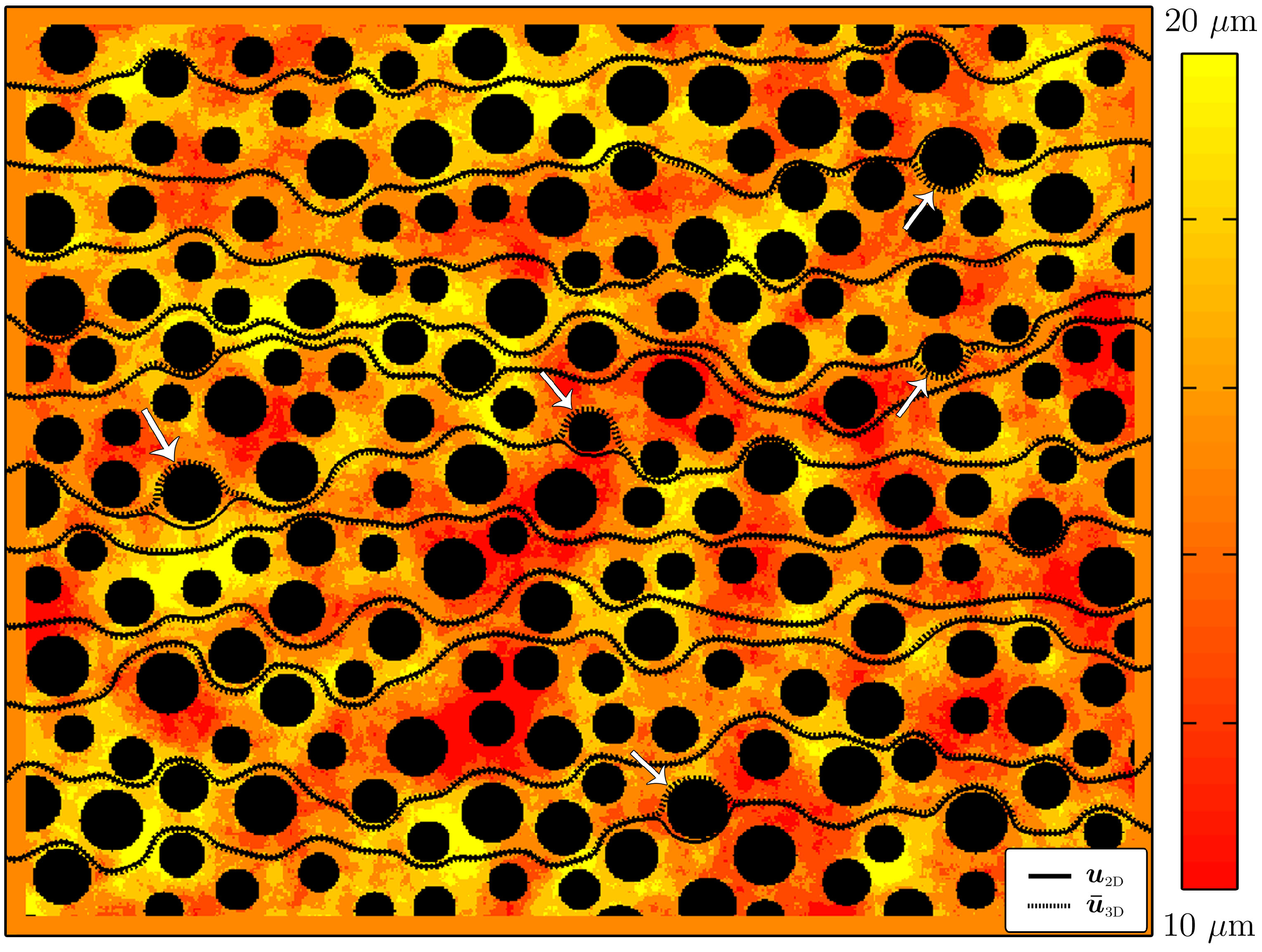
4.3. Heterogeneous Pore Geometry

In a heterogeneous pore geometry of cylindrical pillars, streamlines of $u_{2D}(x,y)$ and ${\overline{u}}_{3D}(x,y)$ are generally close. At five locations, indicated by arrows in Figure 6, streamlines diverge just upstream of a pillar, travel around it on opposite sides, and reconnect just downstream of the pillar. Agreement between streamlines downstream of these errors appears unaffected, suggesting that error does not propagate. The divergence of streamlines around pillars may be caused by differing position of the stagnation point in $u_{2D}(x,y)$ and ${\overline{u}}_{3D}(x,y)$. This error does not appear in our simulations with uniform aperture, in which streamlines near pillars suggest the stagnation point is positioned as theory would predict [32] (Chapter 6.9). Streamline error may depend on properties of the porous medium, such as its permeability, porosity, and the shape of grains. Even with these properties kept constant, different arrangements of grains may yield different results. Because streamline error appears mostly localized near grains, we may reason that for a fixed porosity, porous media with a larger number of grains are more likely to suffer from the streamline error shown in Figure 6. In that pore geometry, streamlines diverge around both small and large grains. It is unclear if there is a trend between grain size and local error. Further investigation is needed to elucidate limitations of the proposed model with respect to porous medium properties. The example presented in Figure 6 serves as a proof of concept for application of the proposed 2D method in a larger and more complex geometry.

Normalized RMSE is 0.0094 and 0.0069 for $u_{2D}(x,y)$ and $v_{2D}(x,y)$, respectively, with a speedup of 40.5. In comparison with other test cases, we observe the greatest discrepancy in streamlines but not the greatest RMSE values for $u_{2D}(x,y)$ in the heterogeneous pore geometry, suggesting normalized RMSE may not be a good indicator of streamline error. This result is reasonable, because the RMSE measures error over the entire velocity field, while streamline error appears to be a more local phenomenon.

Computed permeability yields an 11% error (see Table 1) for the large heterogeneous pore geometry. Recall $\theta =0.087$ for this geometry, and for the unit cell with $\theta =0.093$ error in permeability was about 12%. The similarity of these figures suggests permeability error may not depend strongly on domain size, considering the heterogeneous geometry has an area nearly four times larger than the unit cell. This observation bodes well for the proposed method’s scalability.

Figure 6. Streamlines of $u_{2D}(x,y)$ and ${\overline{u}}_{3D}(x,y)$ in a heterogeneous pore geometry. Aperture is a spatially-correlated random field between 10 and 20 μm, shown as color map, with an aperture covariance range of $\theta \approx 0.09$ (as a fraction of the geometry’s length). Arrows indicate locations where streamlines diverge around grains.

Figure 6. Streamlines of $u_{2D}(x,y)$ and ${\overline{u}}_{3D}(x,y)$ in a heterogeneous pore geometry. Aperture is a spatially-correlated random field between 10 and 20 μm, shown as color map, with an aperture covariance range of $\theta \approx 0.09$ (as a fraction of the geometry’s length). Arrows indicate locations where streamlines diverge around grains.

5. Conclusions

In this work, a 2D depth-averaged LBM is presented to approximate the depth-averaged results of a 3D LBM in micromodels with variable aperture, created by impermeable precipitate or biomass. The key ingredient in the 2D approximation is an external body force that approximates the viscous drag imparted on the fluid by the top and bottom micromodel surfaces, which are typically omitted in 2D simulations. We show that this viscous drag term orients the velocity field, taking into account local variation in aperture, which does not occur with the uniform scaling procedure implemented in previous work. Applicability of the proposed method to reactive transport models is judged mainly by the accuracy of streamlines it produces. In unit cells, streamlines agreed strongly with those of the depth-averaged 3D velocity field. In the larger domain, streamlines sometimes diverged around cylindrical obstructions. This discrepancy did not appear to propagate downstream, as streamlines soon reconnected. For this reason, the proposed 2D method appears appropriate for applications in reactive transport in large porous domains, provided some local error near grains is acceptable. More precisely, in the case of surface reactions [33] with advection-dominated transport, i.e., large Peclet number, results are likely to be highly sensitive to velocities near grain boundaries. In this scenario, the aforementioned local error may be problematic. Permeabilities computed by the proposed method were accurate to within approximately 10% but required about 40 times less CPU run time to compute than from a fully 3D method. Error in permeability can be attributed to sources of drag that are not accounted for by the 2D method, such as drag from vertically-oriented surfaces, as well as reduced validity of the model’s assumptions. For test cases considered in this work, the proposed 2D method captured the permeability and depth-averaged velocity field of a fully 3D method with reasonable accuracy, while significantly reducing computational expense.

References

1. Boyd, V.; Yoon, H.; Zhang, C.; Oostrom, M.; Hess, N.; Fouke, B.; Valocchi, A.J.; Werth, C.J. Influence of Mg2+ on CaCO3 precipitation during subsurface reactive transport in a homogeneous silicon-etched pore network. Geochim. Cosmochim. Acta 2014, 135, 321–335. [Google Scholar] [CrossRef]
2. Zhang, C.; Dehoff, K.; Hess, N.; Oostrom, M.; Wietsma, T.W.; Valocchi, A.J.; Fouke, B.W.; Werth, C.J. Pore-Scale Study of Transverse Mixing Induced CaCO3 Precipitation and Permeability Reduction in a Model Subsurface Sedimentary System. Environ. Sci. Technol. 2010, 44, 7833–7838. [Google Scholar] [CrossRef] [PubMed]
3. Willingham, T.W.; Werth, C.J.; Valocchi, A.J. Evaluation of the Effects of Porous Media Structure on Mixing-Controlled Reactions Using Pore-Scale Modeling and Micromodel Experiments. Environ. Sci. Technol. 2008, 42, 3185–3193. [Google Scholar] [CrossRef] [PubMed]
4. Yoon, H.; Valocchi, A.J.; Werth, C.J.; Dewers, T. Pore-scale simulation of mixing-induced calcium carbonate precipitation and dissolution in a microfluidic pore network. Water Resour. Res. 2012, 48. [Google Scholar] [CrossRef]
5. Knutson, C.E.; Werth, C.J.; Valocchi, A.J. Pore-scale simulation of biomass growth along the transverse mixing zone of a model two-dimensional porous medium. Water Resour. Res. 2005, 41. [Google Scholar] [CrossRef]
6. Tang, Y.; Valocchi, A.J.; Werth, C.J.; Liu, H. An improved pore-scale biofilm model and comparison with a microfluidic flow cell experiment. Water Resour. Res. 2013, 49, 8370–8382. [Google Scholar] [CrossRef]
7. Willingham, T.; Zhang, C.; Werth, C.J.; Valocchi, A.J.; Oostrom, M.; Wietsma, T.W. Using dispersivity values to quantify the effects of pore-scale flow focusing on enhanced reaction along a transverse mixing zone. Adv. Water Resour. 2010, 33, 525–535. [Google Scholar] [CrossRef]
8. Venturoli, M.; Boek, E.S. Two-dimensional lattice-Boltzmann simulations of single phase flow in a pseudo two-dimensional micromodel. Phys. A Stat. Mech. Appl. 2006, 362, 23–29. [Google Scholar] [CrossRef]
9. Boek, E.S.; Venturoli, M. Lattice-Boltzmann Studies of Fluid Flow in Porous Media with Realistic Rock Geometries. Comput. Math. Appl. 2010, 59, 2305–2314. [Google Scholar] [CrossRef]
10. Stewart, M.; Ward, A.; Rector, D. A study of pore geometry effects on anisotropy in hydraulic permeability using the lattice-Boltzmann method. Adv. Water Resour. 2006, 29, 1328–1340. [Google Scholar] [CrossRef]
11. Harting, J.; Kunert, C.; Hyvaluoma, J. Lattice Boltzmann simulations in microfluidics: Probing the no-slip boundary condition in hydrophobic, rough, and surface nanobubble laden microchannels. Microfluid. Nanofluid. 2010, 8, 1–10. [Google Scholar] [CrossRef]
12. Karlin, I.; Bosch, F.; Chikatamarla, S. Gibbs’ principle for the lattice-kinetic theory of fluid dynamics. Phys. Rev. E 2014, 90, 031302. [Google Scholar] [CrossRef] [PubMed]
13. Pan, C.; Luo, L.S.; Miller, C.T. An evaluation of lattice Boltzmann schemes for porous medium flow simulation. Comput. Fluid. 2006, 35, 898–909. [Google Scholar] [CrossRef]
14. Talon, L.; Bauer, D.; Gland, N.; Youssef, S.; Auradou, H.; Ginzburg, I. Assessment of the two relaxation time Lattice-Boltzmann scheme to simulate Stokes flow in porous media. Water Resour. Res. 2012, 48. [Google Scholar] [CrossRef]
15. Oron, A.; Davis, S.H.; Bankoff, S.G. Long-scale evolution of thin liquid films. Rev. Mod. Phys. 1997, 69, 931–980. [Google Scholar] [CrossRef]
16. White, F.M. Viscous Fluid Flow, 2nd ed.; McGraw-Hill: New York, NY, USA, 1991. [Google Scholar]
17. Brush, D.J.; Thomson, N.R. Fluid Flow in Synthetic Rough-Walled Fractures: Navier-Stokes, Stokes, and Local Cubic Law Simulations. Water Resour. Res. 2003, 39. [Google Scholar] [CrossRef]
18. Flekkøy, E.G.; Oxaal, U.; Feder, J.; Jøssang, T. Hydrodynamic dispersion at stagnation points: Simulations and experiments. Phys. Rev. E 1995, 52, 4952–4962. [Google Scholar] [CrossRef]
19. Succi, S. The Lattice Boltzmann Equation for Fluid Dynamics and Beyond; Oxford University Press: Oxford, UK, 2001. [Google Scholar]
20. Bhatnagar, P.L.; Gross, E.P.; Krook, M. A Model for Collision Processes in Gases. I. Small Amplitude Processes in Charged and Neutral One-Component Systems. Phys. Rev. 1954, 94, 511–525. [Google Scholar] [CrossRef]
21. Guo, Z.; Shu, C. Lattice Boltzmann Method and Its Applications in Engineering; World Scientific Publishing Co.: Singapore, 2013. [Google Scholar]
22. d’Humieres, D.; Ginzburg, I.; Krafczyk, M.; Lallemand, P.; Luo, L.S. Multiple-relaxation-time lattice Boltzmann models in three dimensions. Philos. Trans. R. Soc. Lond. Ser. A Math. Phys. Eng. Sci. 2002, 360, 437–451. [Google Scholar] [CrossRef] [PubMed]
23. McCracken, M.E.; Abraham, J. Multiple-relaxation-time lattice-Boltzmann model for multiphase flow. Phys. Rev. E 2005, 71, 036701. [Google Scholar] [CrossRef] [PubMed]
24. Zou, Q.; Hou, S.; Chen, S.; Doolen, G. An improved incompressible lattice Boltzmann model for time-independent flows. J. Stat. Phys. 1995, 81, 35–48. [Google Scholar] [CrossRef]
25. Guo, Z.; Zheng, C.; Shi, B. Discrete lattice effects on the forcing term in the lattice Boltzmann method. Phys. Rev. E 2002, 65, 046308. [Google Scholar] [CrossRef] [PubMed]
26. Hou, S.; Zou, Q.; Chen, S.; Doolen, G.; Cogley, A.C. Simulation of Cavity Flow by the Lattice Boltzmann Method. J. Comput. Phys. 1995, 118, 329–347. [Google Scholar] [CrossRef]
27. Kozintsev, B. Computations with Gaussian Random Fields. Ph.D. Thesis, University of Maryland, College Park, MD, USA, 1999. [Google Scholar]
28. Neuville, A.; Flekkøy, E.; Toussaint, R. Influence of asperities on fluid and thermal flow in a fracture: A coupled lattice Boltzmann study. J. Geophys. Res. Solid Earth 2013, 118, 3394–3407. [Google Scholar] [CrossRef] [Green Version]
29. Clipped Gaussian Random Fields. Available online: http://math4411.math.umd.edu/cgi-bin/bak/generate.cgi/ (acccessed on 23 November 2015).
30. Bouzidi, M.; d’Humieres, D.; Lallemand, P.; Luo, L.S. Lattice Boltzmann Equation on a Two-Dimensional Rectangular Grid. J. Comput. Phys. 2001, 172, 704–717. [Google Scholar] [CrossRef]
31. Sukop, M.C.; Thorne, D.T. Lattice Boltzmann Modeling: An Introduction for Geoscientists and Engineers, 1st ed.; Springer Publishing Company: Berlin, Germany, 2010. [Google Scholar]
32. Kundu, P.K.; Cohen, I.M. Fluid Mechanics, 4th ed.; Elsevier: Burlington, VT, USA, 2008. [Google Scholar]
33. Hiorth, A.; Jettestuen, E.; Cathles, L.; Madland, M. Precipitation, dissolution, and ion exchange processes coupled with a lattice Boltzmann advection diffusion solver. Geochim. Cosmochim. Acta 2013, 104, 99–110. [Google Scholar] [CrossRef]