Numerical Simulation of Fluid-Solid Coupling in Fractured Porous Media with Discrete Fracture Model and Extended Finite Element Method

Abstract

Fluid-solid coupling is ubiquitous in the process of fluid flow underground and has a significant influence on the development of oil and gas reservoirs. To investigate these phenomena, the coupled mathematical model of solid deformation and fluid flow in fractured porous media is established. In this study, the discrete fracture model (DFM) is applied to capture fluid flow in the fractured porous media, which represents fractures explicitly and avoids calculating shape factor for cross flow. In addition, the extended finite element method (XFEM) is applied to capture solid deformation due to the discontinuity caused by fractures. More importantly, this model captures the change of fractures aperture during the simulation, and then adjusts fluid flow in the fractures. The final linear equation set is derived and solved for a 2D plane strain problem. Results show that the combination of discrete fracture model and extended finite element method is suited for simulating coupled deformation and fluid flow in fractured porous media.

1. Introduction

The technology of hydraulic fracturing has been widely used for reservoir stimulation, especially for unconventional reservoirs [1]. Coupled rock deformation and fluid flow in fractured porous media is important for reservoir simulation because rock deformation exerts an important influence on reservoir production [2].

The general theory of 3D consolidation with elasticity constitutive relationship and Darcy’ law has been established by Biot [3], and the effective stress formulation has been put forward by Terzaghi [4]. A great number of researches about fluid-solid coupling have been done based on these theories in petroleum engineering, from conventional reservoirs to fractured reservoirs [5].

There exist several methods to simulate fluid flow in fractured porous media [6]. Warren and Root introduced the dual continuum concept to characterize naturally fractured reservoirs [7]. The dual continuum approaches treat fracture and matrix both as continua distributed within reservoir domain. The fracture-matrix cross flow is based on the analytical solution of pseudosteady-state flow within the matrix system with a simple geometry of matrix blocks. Moreover, shape factors are calculated for different geometries of matrix blocks. The dual continuum approaches consist of dual porosity and dual permeability models [8]. Schematics for dual porosity concept and dual permeability concept are shown in Figure 1 and Figure 2 respectively. The difference between dual porosity model and dual permeability model is that dual permeability model takes global matrix-matrix flow into account while dual porosity model does not account for it.

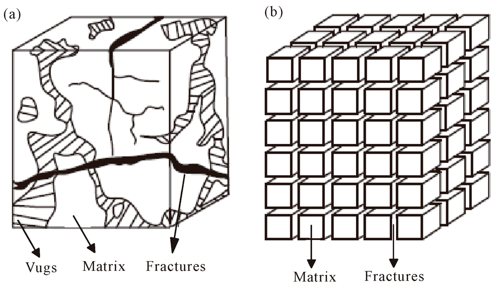
Figure 1. Schematic illustration of dual porosity model of fractured reservoirs. (a) Actual reservoir; (b) Reservoir model.

Figure 1. Schematic illustration of dual porosity model of fractured reservoirs. (a) Actual reservoir; (b) Reservoir model.

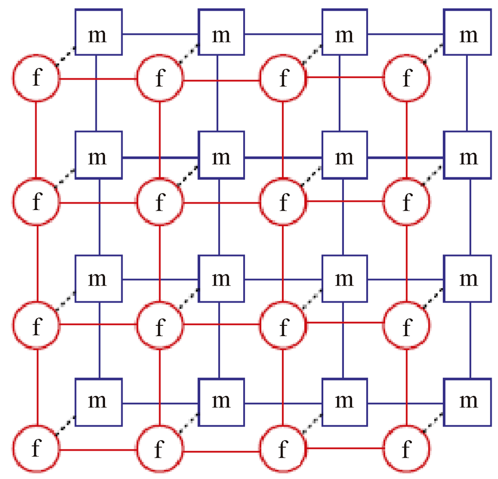
Figure 2. Schematic illustration of dual permeability model of fractured reservoirs.

Figure 2. Schematic illustration of dual permeability model of fractured reservoirs.

An alternative to the dual continuum approaches is the discrete fracture model [9,10]. The fractures are represented explicitly within the domain and discretized along with the matrix domain. Lamb [11] presented fracture mapping approach (FM) to simulate fluid flow in fractured porous media. In the FM approach, an element intersected by a fracture is treated as a superposition of two elements, namely a matrix element and a fracture element. The matrix element and fracture element interact via a transfer function. The schematic of fracture mapping approach is shown in Figure 3. The approach adopts the transfer function presented by Barenblatt [12] to account for cross flow between the overlapping matrix and fracture elements, which was a dual continuum model to this extent.

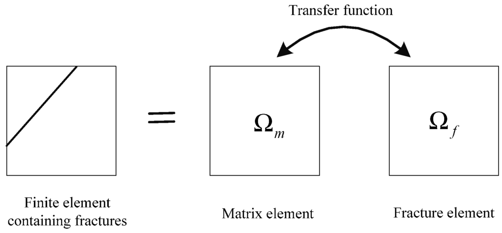
Figure 3. Schematic representation of fracture mapping approach (FM).

Figure 3. Schematic representation of fracture mapping approach (FM).

Due to stress singularity of fracture tip, it needs mesh refinement around the fracture in the standard finite element framework, which is computational burdensome. An alternative to standard finite element method is the extended finite element method (XFEM). The extended finite element method was introduced by Belytschko [13] to discontinuous problems, which has been widely used in many fields due to flexibility in meshing [14,15,16,17]. The fracture is represented by level set method.

Ghafouri and Lewis [18,19] presented a finite element continuum approach to describe the coupled deformation and fluid flow in fractured porous media, which was based on double porosity model. Tran [20] presented high level boundary element method with periodic boundary conditions and flux continuous finite volume element method to simulate coupled fluid flow through discrete fracture network; Al-Khoury [21] used the partition of unity method to describe the fracturing process and double porosity model to describe the resulting fluid flow; Vire et al. [22] presented coupling an adaptive mesh finite element fluid model with a combined finite-discrete element solid model to investigate fluid-solid interactions. The method is flexible in terms of discretization schemes used for each material. Recently, Vire et al. [23] presents an immersed-shell method for modeling fluid-structure interactions. The method consists of immersing the solid structures in an extended fluid domain, and exchanging the coupling forces through a thin shell surrounding the solid structures. Lamb [13] presented FM approach and the extended finite element method for coupled deformation and fluid flow in fractured porous media. The difference between this paper and Lamb’s is that here discrete fracture model is used to avoid calculating cross flow and the model captures the change of fractures aperture during the simulation.

The advantages of combination of discrete fracture model and extended finite element method over other methods are that discrete fracture model avoids the computation of shape factor and is more accurate than dual continuum model for simulating fluid flow with large fractures, meanwhile the extended finite element method avoids mesh refinement around the fracture and is well suited for discontinuity problems. Furthermore, the model is capable of capturing change of fractures aperture during the simulation.

In this paper, the combination of discrete fracture model and extended finite element method is used to couple deformation and fluid flow in fractured porous media. The governing equations and initial and boundary conditions are presented in Section 2. The numerical solution is presented in Section 3. In the section, the extended finite element method and the discrete fracture model are briefly described to capture deformation and fluid flow respectively, and spatial and temporal discretization are conducted. Finally, numerical simulation and result analysis are performed in Section 4 and the conclusion are drawn in Section 5.

2. Mathematical Model

2.1. Governing Equations for Rock Deformation

Under the assumptions of small-strain situation, isothermal equilibrium and negligible inertial forces, Biot’s theory describes the linear momentum balance equation for a two-phase medium, which is composed by rock and water.

$${\nabla }_s^{\text{T}}\mathit{\sigma }+\rho \mathit{g}=0$$

(1)

where $\mathit{\sigma }$ is total stress tensor, $\mathit{g}$ is gravity, $\rho$ is the averaged density of the multiphase system, and ${\nabla }_s^{\text{T}}$ is the symmetric gradient operator matrix.

$$\rho =(1-\varphi ){\rho }^s+\varphi {\rho }^w$$

(2)

$${\nabla }_s=\left[\begin{array}{cc}\begin{array}{l}\raisebox{1ex}{$\partial $}\!\left/ \!\raisebox{-1ex}{$\partial x$}\right.\\ 0\\ \raisebox{1ex}{$\partial $}\!\left/ \!\raisebox{-1ex}{$\partial y$}\right.\end{array}& \begin{array}{l}0\\ \raisebox{1ex}{$\partial $}\!\left/ \!\raisebox{-1ex}{$\partial y$}\right.\\ \raisebox{1ex}{$\partial $}\!\left/ \!\raisebox{-1ex}{$\partial x$}\right.\end{array}\end{array}\right]$$

(3)

where $\varphi$ is porosity, ${\rho }^s$ is the density of solid, and ${\rho }^w$ is the density of water.

The relationship between total stress and effective stress is given by

$$\mathit{\sigma }={\mathit{\sigma }}^{\mathbf{e}}-\alpha \mathit{m}{p}^w$$

(4)

where ${\mathit{\sigma }}^e$ is the effective stress, $p^w$ is the water pore pressure in the porous matrix, $\alpha$ is the Biot’s compressibility coefficient, and $\mathit{m}={[110]}^{\text{T}}$ in two dimensions.

The constitutive stress-strain relationship of the solid phase is given by

$$\mathit{\sigma }=\mathit{D}\mathit{\epsilon }$$

(5)

where D is the linear elastic material matrix and $\mathit{\epsilon }$ is the strain of the system.

The geometric equation between strain and displacement is given by

$$\mathit{\epsilon }={\nabla }_s\mathit{u}$$

(6)

where u is the displacement of the system.

2.2. Governing Equations for Fluid Flow

Fluid flow in fractured porous media is typically simulated using dual-porosity models, but dual-porosity models are not well suited for the modeling of a small number of large-scale fractures, which may dominate the flow. Discrete fracture model, in which the fractures are represented individually, has been broadly applied to simulate flow in fractured porous media. In this paper, discrete fracture model is used for flow simulation.

The equation of motion for fluid flow in porous media is given by Darcy’ law as follows

$$\mathit{v}=-\frac{k}{{\mu }_w}(\nabla p^w-{\rho }^w\mathit{g})$$

(7)

where $\mathit{v}$ is velocity, $k$ is permeability, ${\mu }_w$ is viscosity of water.

The continuity equation takes into consideration the grain and fluid volume variation resulting from pressure change (the first term) and total volume strain resulting from solid deformation (the second term), which is given by

$$(\frac{\alpha -\varphi }{K_s}+\frac{\varphi }{K_w})\frac{\partial p^w}{\partial t}+\alpha {\mathit{m}}^{\text{T}}\frac{\partial \mathit{\epsilon }}{\partial t}+\nabla \cdot [\frac{k}{{\mu }_w}(-\nabla p^w+{\rho }^w\mathit{g})]=0$$

(8)

where $K_s$ is the bulk modulus of the grain material, $K_w$ is the bulk modulus of water.

2.3. Initial and Boundary Conditions

The initial conditions specify the displacement and water pressure fields at time $t=0$.

$$\mathit{u}={\mathit{u}}_0,p^w=p_0^w\text{ in }\Omega \text{ and on }\Gamma$$

(9)

where Ω is the domain of interest and Γ is the boundary.

Boundary conditions of solid deformation include displacement condition and force condition, which can be given as follows

$$\{\begin{array}{l}\mathit{u}=\overline{\mathit{u}}on{\Gamma }_u\\ {\mathit{l}}^{\text{T}}\mathit{\sigma }=\overline{\mathit{t}}on{\text{Γ}}_t\end{array}$$

(10)

where $\mathit{l}$ is related to the unit outward normal vector $\mathit{n}={\{n_x,n_y\}}^{\text{T}}$ by

$$\mathit{l}=\left[\begin{array}{cc}\begin{array}{l}{n}_x\\ 0\\ n_y\end{array}& \begin{array}{l}0\\ n_y\\ n_x\end{array}\end{array}\right]$$

(11)

Boundary conditions of fluid flow include water pressure condition and flux condition, which can be given as follows

$$\{\begin{array}{l}{p}^w=\overline{p}on{\text{Γ}}_p\\ \frac{k}{{\mu }_w}{(-\nabla p^w+{\rho }^w\mathit{g})}^{\text{T}}=q^w\text{ on }{\text{Γ}}_q\end{array}$$

(12)

where $q^w$ is the imposed volume flux normal to the boundary.

3. Numerical Solution

3.1. Application of the Extended Finite Element Method

In the finite element framework, discontinuity modeling needs mesh refinement around the crack, which is computationally burdensome. The extended finite element method was introduced by Belytschko and Black, which had been widely used for discontinuous problem. The advantage of extended finite element method is avoiding mesh refinement around fractures (especially fracture tips) without reducing accuracy. The method is adopted to solve solid deformation in this study.

The extended finite element method exploits the partition of unity property of finite element. The displacement field is decomposed into two parts: the continuous displacement field and the discontinuous part. The displacement approximation can be written as follows

$${\mathit{u}}^h(\mathit{x})={\displaystyle \sum _{I\in N}{N}_I(\mathit{x}){\mathit{u}}_I+}{\displaystyle \sum _{I\in N^{cr}}{N}_I(\mathit{x})(H(\varphi (\mathit{x}))-H(\varphi ({\mathit{x}}_I))){\mathit{a}}_I}+{\displaystyle \sum _{I\in N^{tip}}{N}_I(\mathit{x}){\displaystyle \sum _{k=1}^4({\text{Φ}}_{\gamma }(\mathit{x})-{\text{Φ}}_{\gamma }({\mathit{x}}_I))}{\mathit{b}}_I^k}$$

(13)

where $\mathit{x}$ is the position vector; ${\mathit{u}}_I$ is the nodal displacements; $N_I$ is the shape function for non-enriched and enriched nodes, respectively; ${\mathit{a}}_I$ and ${\mathit{b}}_I^k$ are degrees for enriched nodes; $H(\xi )$ is Heaviside step function; $\varphi (\mathit{x})$ is signed distance function; ${\text{Φ}}_{\gamma }(\mathit{x})$ is enriched functions for tip elements; $N$ is the set of all nodes in discretized model; $N^{cr}$ is the set of nodes of all elements containing cracks but not crack tips; $N^{tip}$ is the set of nodes of all elements containing the crack tip.

Heaviside step function is defined as

$$H(x)=\{\begin{array}{l}1,x>0\\ 0,x=0\\ -1,x<0\end{array}$$

(14)

From Equation (13), the opening between the two surfaces of the fracture can be given by

$$\Vert \mathit{u}\Vert =\mathit{n}\cdot ({\mathit{u}}^{+}-{\mathit{u}}^{-})=2\mathit{n}\cdot {\displaystyle \sum _{I\in N^{cr}}{N}_I}{\mathit{a}}_I+2\mathit{n}\cdot \sqrt{r}{\displaystyle \sum _{I\in N^{tip}}{N}_I}{\mathit{b}}_I^1$$

(15)

where $\mathit{n}$ is the unit outward normal vector.

3.2. Application of Discrete Fracture Model

In discrete fracture model, fractures are simplified into 1D line element for 2D problem, and 2D surface area element for 3D problem, as shown in Figure 4. The whole fractured porous media is decomposed into two parts: matrix system and fracture system, which can be given as follows

$$\text{Ω}={\text{Ω}}_m+a{\text{Ω}}_f$$

(16)

where $m$ represents matrix, $f$ represents fracture, and $a$ is the aperture of fracture.

Assuming that representative element volumes of both matrix and fracture system exist, flow equations are applicable to the whole research region. Then for the discrete fracture model, the integral form of the flow equation can be given as follows.

$${\displaystyle {\int }_{\text{Ω}}F}d\text{Ω}={\displaystyle {\int }_{{\text{Ω}}_m}F}d{\text{Ω}}_m+{\displaystyle {\int }_{{\text{Ω}}_f}aF}d{\text{Ω}}_f$$

(17)

In the Equations (16) and (17), the apertures of fractures are calculated from Equation (15). In the implementation of algorithm, fractures are discretized into small segments. Moreover, the aperture of each segment is set equal to average opening of its endpoints, which is easy to calculate from Equation (15). However, the initial aperture of fracture is given in the first time step and updated from the second time step.

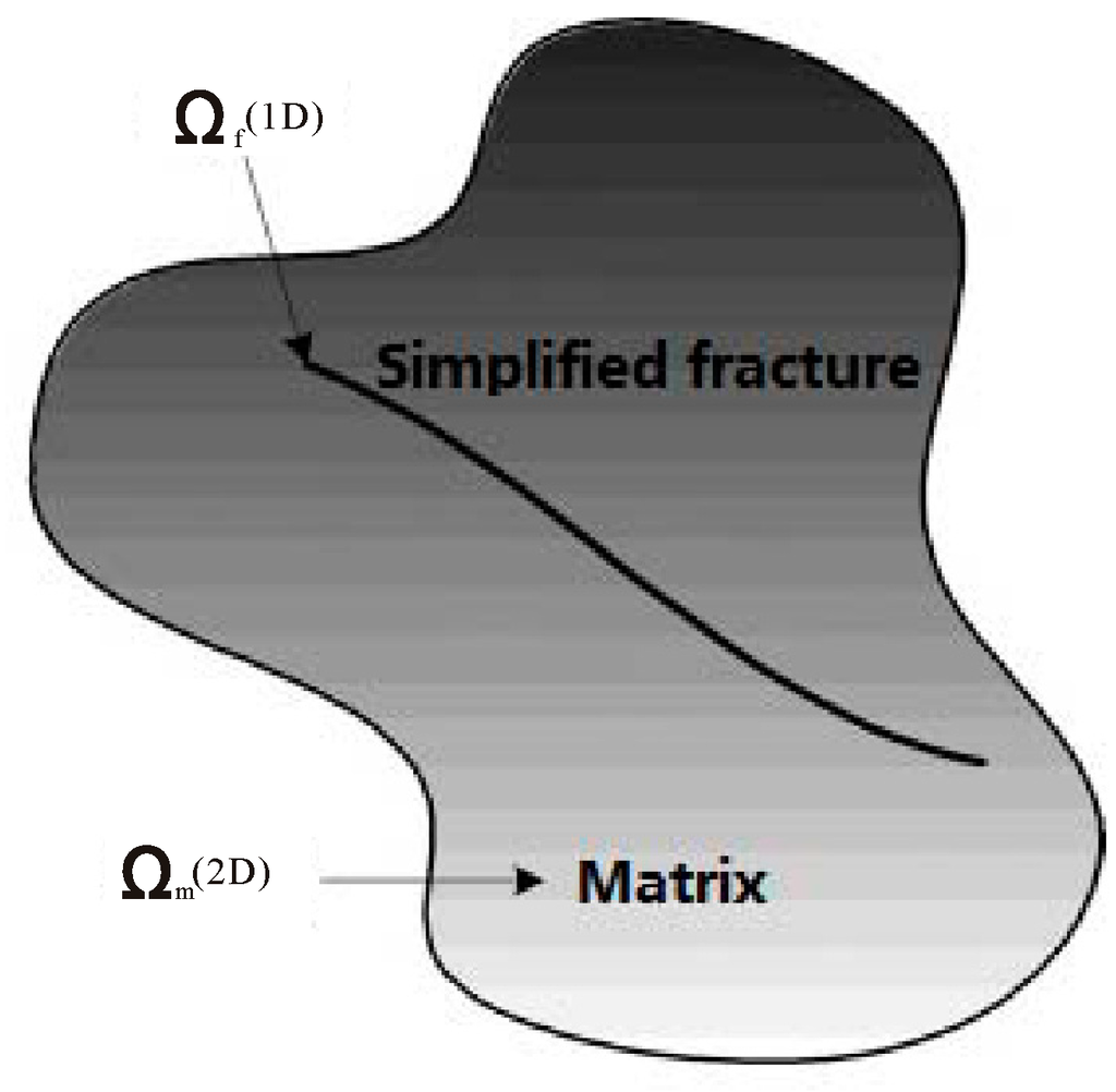
Figure 4. Schematic of a discrete fracture model.

Figure 4. Schematic of a discrete fracture model.

3.3. Discretization in Space

According to strong form of solid deformation equation, the weak form can be expressed with weighted residual method

$${\displaystyle {\int }_{\text{Ω}}\mathit{\epsilon }(\mathit{u})}:\mathit{D}:\mathit{\epsilon }(\mathit{v})\text{dΩ}-\alpha {\displaystyle {\int }_{\text{Ω}}{\mathit{\epsilon }}^{\text{T}}(\mathit{v})\cdot \mathit{m}{p}^w\text{dΩ}={\displaystyle {\int }_{\text{Ω}}\rho \mathit{g}\cdot \mathit{v}}\text{dΩ}+{\displaystyle {\int }_{{\text{Γ}}_t}\overline{\mathit{t}}}}\cdot \mathit{v}\text{dΓ},\forall \mathit{v}\in {\mathit{U}}_0$$

(18)

where ${\mathit{U}}_0=\left\{\mathit{v}\right|\mathit{v}\in {\mathit{C}}^0(\text{Ω}/{\text{Γ}}_{cr}),\mathit{v}{|}_{{\text{Γ}}_u}=\mathbf{0}\}$ is the trial function space, and ${\text{Γ}}_{cr}$ is the fracture in the domain.

The weighted residual method is applied to the continuity equation for water flow and to its natural boundary condition, which yields

$${\displaystyle {\int }_{\text{Ω}}\nabla w}\cdot (\frac{k_m}{{\mu }_w}\nabla p^w-{\rho }^w\mathit{g})+w\cdot \alpha \mathit{m}{\nabla }_s\frac{\partial \mathit{u}}{\partial t}+w(\frac{\alpha -\varphi }{K_s}+\frac{\varphi }{K_w})\frac{\partial p^w}{\partial t}\text{dΩ}+{\displaystyle {\int }_{{\text{Γ}}_q}w}\cdot q^w\text{dΓ}=0$$

(19)

where $w$ is the weight function, and $\text{Ω}$ is the region of integration expressed by Equation (16), which consists of matrix and fracture system. Equation (19) turns to

$$\begin{array}{l}{\displaystyle {\int }_{{\text{Ω}}_m}\nabla w}\cdot (\frac{k_m}{{\mu }_w}\nabla p^w-{\rho }^w\mathit{g})+w\cdot \alpha \mathit{m}{\nabla }_s\frac{\partial \mathit{u}}{\partial t}+w(\frac{\alpha -\varphi }{K_s}+\frac{\varphi }{K_w})\frac{\partial p^w}{\partial t}{\text{dΩ}}_m+\\ {\displaystyle {\int }_{{\text{Ω}}_f}a\cdot [\nabla w}\cdot (\frac{k_f}{{\mu }_w}\nabla p^w-{\rho }^w\mathit{g})+w\cdot \alpha \mathit{m}{\nabla }_s\frac{\partial \mathit{u}}{\partial t}+w(\frac{\alpha -\varphi }{K_s}+\frac{\varphi }{K_w})\frac{\partial p^w}{\partial t}]{\text{dΩ}}_f+{\displaystyle {\int }_{{\text{Γ}}_q}w}\cdot q^w\text{dΓ}=0\end{array}$$

(20)

where $k_m$ is the permeability of matrix, and $k_f$ is the permeability of fracture, which can be given by “cubic law” as follows

$$k_f=\frac{a^2}{12}$$

(21)

The expression for displacement is given by Equation (13), and the expression for water pressure is given as follows

$$p^w={\mathit{N}}_p{\overline{\mathit{p}}}^w$$

(22)

where ${\overline{\mathit{p}}}^w$ is the vector of the nodal values of water pressure, and ${\mathit{N}}_p$ is the shape function for water pressure.

By integrating Equations (18) and (20), the weak form of the whole system is discretized into the following set of equations

$$\mathit{A}\mathit{X}+\mathit{B}\frac{\text{d}\mathit{X}}{\text{d}t}=\mathit{C}$$

(23)

where

$$\mathit{A}=\left[\begin{array}{cccc}\mathit{K}{\mathit{e}}_{uu}& \mathit{K}{\mathit{e}}_{ua}& \mathit{K}{\mathit{e}}_{ub}& -{\mathit{L}}_{\mathit{u}}\\ \mathit{K}{\mathit{e}}_{au}& \mathit{K}{\mathit{e}}_{aa}& \mathit{K}{\mathit{e}}_{ab}& -{\mathit{L}}_a\\ \mathit{K}{\mathit{e}}_{bu}& \mathit{K}{\mathit{e}}_{ba}& \mathit{K}{\mathit{e}}_{bb}& -{\mathit{L}}_b\\ 0& 0& 0& {\mathit{H}}_m+a{\mathit{H}}_f\end{array}\right]$$

(24)

$$\mathit{B}=\left[\begin{array}{cccc}0& 0& 0& 0\\ 0& 0& 0& 0\\ 0& 0& 0& 0\\ {\mathit{L}}_{\mathit{u}}^{\text{T}}& {\mathit{L}}_a^{\text{T}}& {\mathit{L}}_b^{\text{T}}& {\mathit{S}}_m+a{\mathit{S}}_f\end{array}\right]$$

(25)

$$\mathit{X}={\text{[}\begin{array}{cccc}\mathit{u}& \mathit{a}& \mathit{b}& {\overline{\mathit{p}}}^w\end{array}\text{]}}^{\text{T}}$$

(26)

$$\mathit{C}={[\begin{array}{cccc}\mathit{F}& {\mathit{F}}_a& {\mathit{F}}_b& \mathit{f}\end{array}]}^{\text{T}}$$

(27)

Elements of the aforementioned listed matrices are given in Appendix.

3.4. Discretization in Time

Using the fully implicit time discretization scheme, the approximation is given as follows

$$\frac{\text{d}\mathit{X}}{\text{d}t}=\frac{{\mathit{X}}_{n+1}-{\mathit{X}}_n}{\text{d}t}$$

(28)

Then, the final discrete equation can be written as follows

$$(\text{d}t\cdot \mathit{A}+\mathit{B}){\mathit{X}}_{n+1}=\mathit{B}{\mathit{X}}_n+\text{d}t\cdot \mathit{C}$$

(29)

The scheme is fully implicit and imposes no requirements of the time step size which is usually chosen for both stability and the elimination oscillatory effects in the solution.

In the above equation, the unknown vector $\mathit{X}$ includes standard degrees of freedom of all nodes, enriched degrees of freedom of enriched nodes in two directions and water pressures of all nodes. The matrices are constructed according to Appendix A and the linear equation set is solved for ${\mathit{X}}_{n+1}$ (value for n + 1 time step) providing that ${\mathit{X}}_n$ (value for n time step) is given. Moreover, the initial value for $\mathit{X}$ is given with the initial conditions by setting nodal displacements and enriched degrees to zero and water pressures to $p_0^w$. The fracture apertures are calculated according to Equation (15) using the already solved displacements, then the matrix for flow in the fracture is updated. The loop continues until end time is reached.

4. Numerical Example

The DFM-XFEM model is applied to a 2D plain strain problem shown in Figure 5. The domain is fully saturated and allowed to freely drain at the top, that is, excess pore water pressure is equal to zero. The domain has an area of 10 m × 16 m. The fracture is 8 m long, is inclined at 45° and is centered in the middle of the domain. The right, left and bottom boundaries are assumed to be undrained. The lateral boundaries of the domain are constrained to vertical translation only, and the bottom boundary is constrained to be fixed. Static load is applied at the top boundary and maintained throughout the duration of the simulation. The input parameters are given in Table 1.

The discrete fracture model has been widely used for simulating flow in fractured porous media, and the extended finite element method has been broadly applied to the discontinuity problem. The combination DFM-XFEM model gives full play to their advantages for simulating flow solid coupling in fractured porous media. The solid module shares the same mesh configuration with the fluid flow module. The numerical method is implemented using Matlab.

Lamb presented fracture mapping approach and the extended finite element method to couple deformation and fluid flow in fractured porous media, denoted by FM-XFEM model. Moreover, the model proposed in this paper is denoted by DFM-XFEM model. Because the fracture geometry remains constant throughout the simulation for the FM-XFEM model, that is, the fracture does not close or open during the simulation, the assumption is applied to the DFM-XFEM model for model verification by comparison with FM-XFEM model. The assumption is done by fixing fracture aperture in the fluid flow module during the simulation. The comparison results of the two models are shown in Figure 6 and Figure 7.

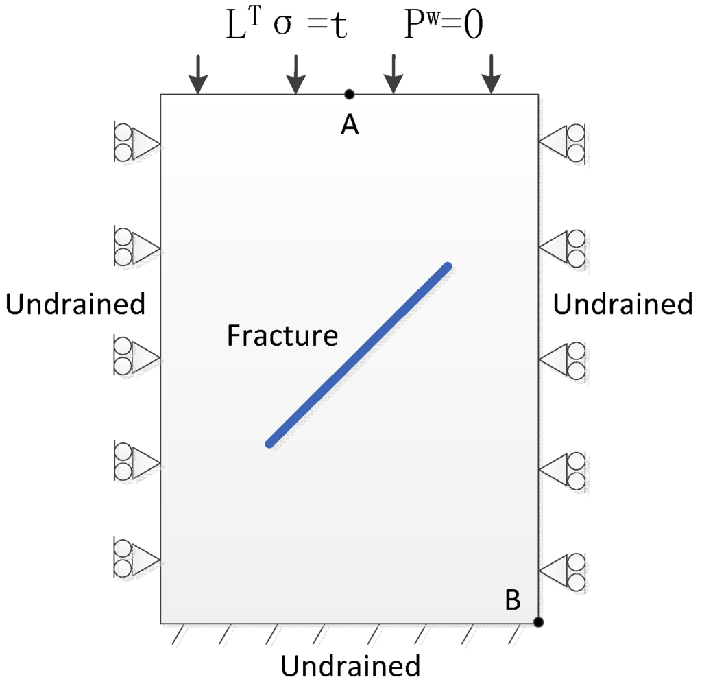
Figure 5. Two-dimensional fractured domain with assigned boundary conditions.

Figure 5. Two-dimensional fractured domain with assigned boundary conditions.

Table 1. Input parameters for the models.

Parameter	Definition	Magnitude	Units
E	Young’s modulus	40	MPa
$v$	Poisson’s ratio	0.3	-
$\mu$	Fluid viscosity	0.001	Pa.s
φm	Matrix porosity	0.1	-
φf	Fracture porosity	0.05	-
km	Matrix permeability	4 × 10−3	Darcy
kf	Fracture permeability	3 × 102	Darcy
Kw	Bulk modulus of fluid	2.0 × 105	MPa
Ks	Bulk modulus of solid	5.0 × 105	MPa
${\overline{t}}_y$	Static load	1.0 × 104	Pa

Table 1. Input parameters for the models.

Parameter	Definition	Magnitude	Units
E	Young’s modulus	40	MPa
$v$	Poisson’s ratio	0.3	-
$\mu$	Fluid viscosity	0.001	Pa.s
φm	Matrix porosity	0.1	-
φf	Fracture porosity	0.05	-
km	Matrix permeability	4 × 10−3	Darcy
kf	Fracture permeability	3 × 102	Darcy
Kw	Bulk modulus of fluid	2.0 × 105	MPa
Ks	Bulk modulus of solid	5.0 × 105	MPa
${\overline{t}}_y$	Static load	1.0 × 104	Pa

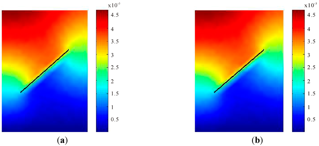
Figure 6. Displacement distribution (m) after 100 days. (a) Fracture mapping extended finite element method (FM-XFEM) model; (b) Discrete fracture model (DFM)-XFEM model.

Figure 6. Displacement distribution (m) after 100 days. (a) Fracture mapping extended finite element method (FM-XFEM) model; (b) Discrete fracture model (DFM)-XFEM model.

Figure 7. Excess pore pressure distribution (Pa) after 100 days. (a) FM-XFEM model; (b) DFM-XFEM model.

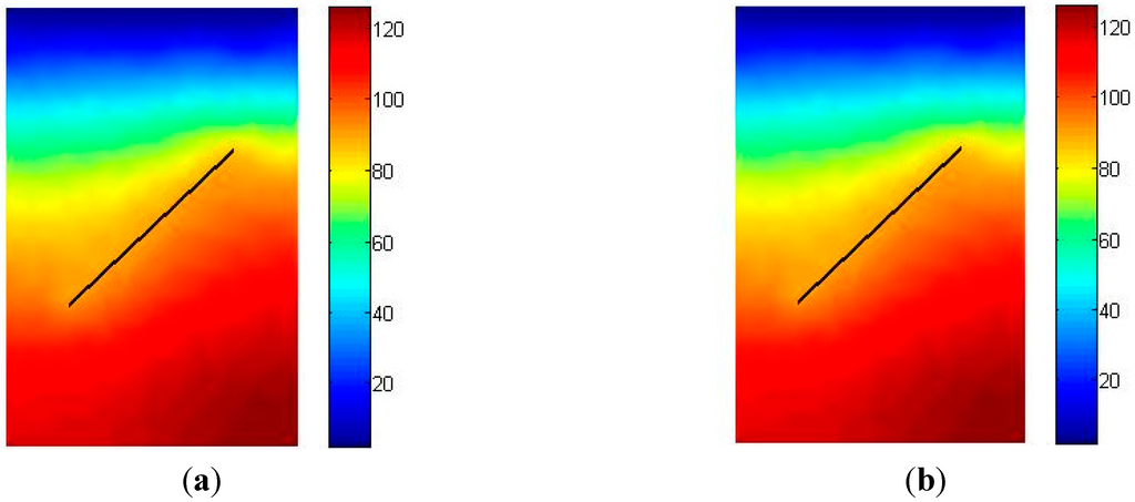
Figure 7. Excess pore pressure distribution (Pa) after 100 days. (a) FM-XFEM model; (b) DFM-XFEM model.

The displacement fields along y direction of the model are shown in Figure 6. The results of two different models are very close, and they are qualitatively identical. The displacement field is discontinuous due to the pre-existing fracture, and the extended finite element method captures discontinuity without mesh refinement around the fracture, which is a great improvement over the standard finite element method.

The excess pore water pressure distributions are shown in Figure 7. The results of two different models are very close, and they are also qualitatively identical. The discrete fracture model represents fracture explicitly, and it does not need to calculate shape factor, which is not easy to determine in the dual porosity model. Because the top boundary is a zero pressure boundary, fluid can freely flow out and the pressure is becoming lower and lower.

The displacement fields along y direction at point A (located at the top shown in Figure 5 and excess pore pressure at point B (located at the bottom shown in Figure 5 for the FM-XFEM model and DFM-XFEM model at varying mesh resolutions during 100 days are shown in Figure 8a and Figure 9a respectively. The plots are zoomed in for 10 days to clarify the discrepancies between the various curves and shown in Figure 8b and Figure 9b. These two figures indicate that the results of DFM-XFEM model show great coincidence with the result of FM-XFEM, which validates the correctness of DFM-XFEM model. Moreover, as the mesh resolutions become higher, the results of DFM-XFEM model show little difference, which validates the convergence of the proposed algorithm.

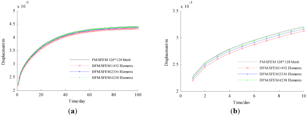
Figure 8. Displacement at point A. (a) 100 days; (b) 10 days.

Figure 8. Displacement at point A. (a) 100 days; (b) 10 days.

Figure 9. Excess pore pressure at point B. (a) 100 days; (b) 10 days.

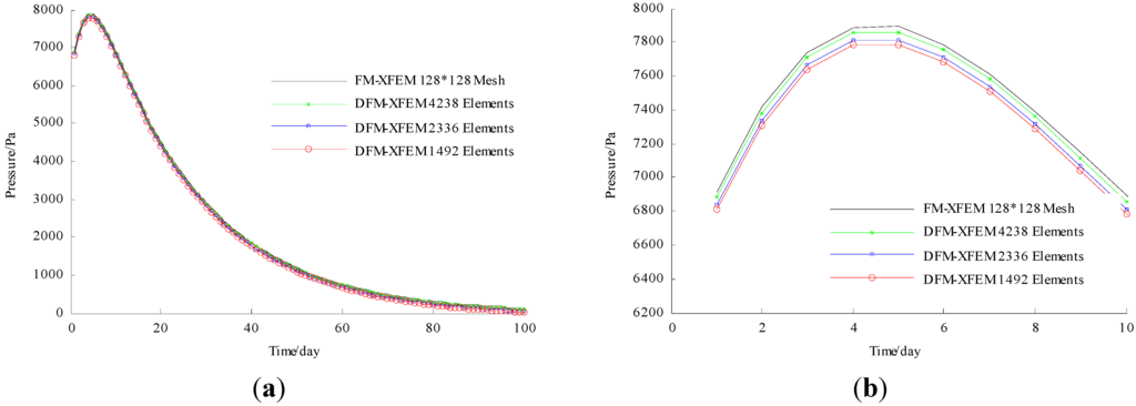
Figure 9. Excess pore pressure at point B. (a) 100 days; (b) 10 days.

The computational cost of models is shown in Table 2. It can be shown that the computational time of DFM-XFEM is much less than that of FM-XFEM with approximately equal number of elements. The comparison shows the advantage of DFM-XFEM over FM-XFEM.

Table 2. Computational cost of models.

Models	Computational Time/s
FM-XFEM 50 × 50 Mesh	31.7
FM-XFEM 70 × 70 Mesh	88.1
DFM-XFEM 1492 Elements	8.8
DFM-XFEM 2336 Elements	14.3
DFM-XFEM 4238 Elements	27.5

Table 2. Computational cost of models.

Models	Computational Time/s
FM-XFEM 50 × 50 Mesh	31.7
FM-XFEM 70 × 70 Mesh	88.1
DFM-XFEM 1492 Elements	8.8
DFM-XFEM 2336 Elements	14.3
DFM-XFEM 4238 Elements	27.5

In the above example, the fracture remains constant during the simulation. However, the fracture could close or open during the simulation, so it needs to capture change of the fracture aperture in the fluid flow. The DFM-XFEM model is able to simulate the situation when fracture aperture changes as described in Section 3.2. The model parameters are the same as the above example. The comparison results for a model with changed and fixed fracture aperture are shown in Figure 10 and Figure 11. Figure 10 illustrates the displacement at point A for 100 days and indicates that the displacement for model with fixed fracture aperture is larger than that for model with changed fracture aperture after a short time and the displacements for these two models show little difference after 50 days. Figure 11 illustrates the excess pore pressure at point B for 100 days and indicates that excess pore pressure for a model with fixed fracture aperture is larger than that for model with changed fracture aperture after a short time and excess pore pressures for these two models show little difference after 50 days. These results are seen because the fracture aperture is becoming smaller, as shown in Figure 12. Figure 12 shows that the fracture aperture decreases quickly after a short time and slows down the decreasing rate after a longer time. As the fracture aperture decreases, the fracture conductivity decreases, which results in pore pressure decreasing more slowly.

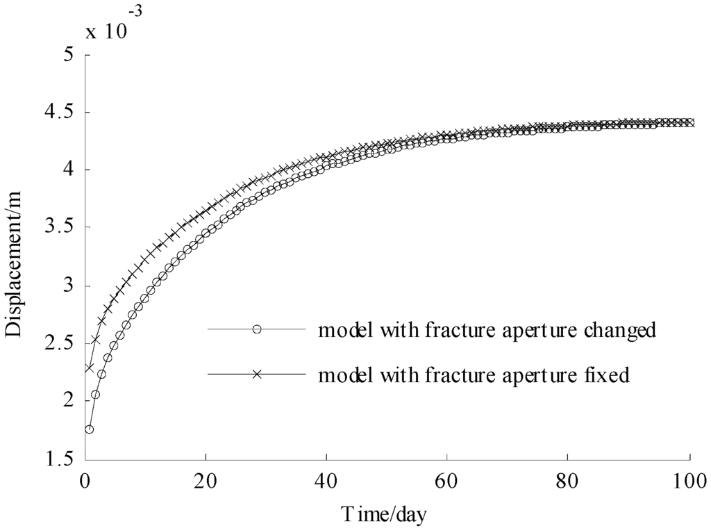
Figure 10. Displacement at point A for 100 days.

Figure 10. Displacement at point A for 100 days.

Figure 11. Excess pore pressure at point B for 100 days.

Figure 11. Excess pore pressure at point B for 100 days.

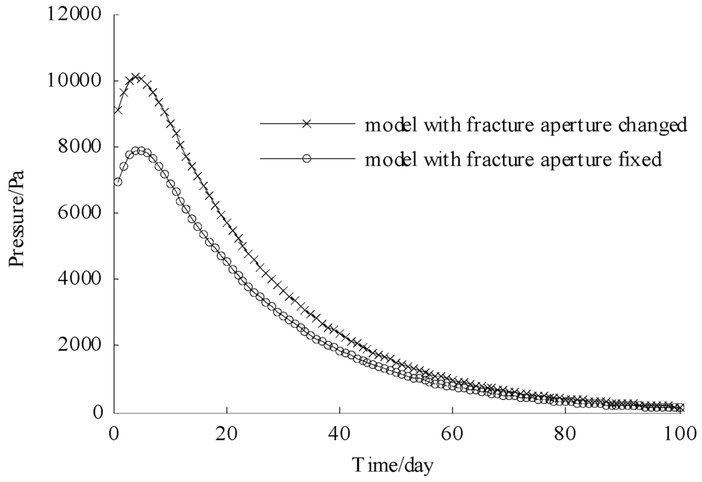
Figure 12. Fracture aperture distribution at different time.

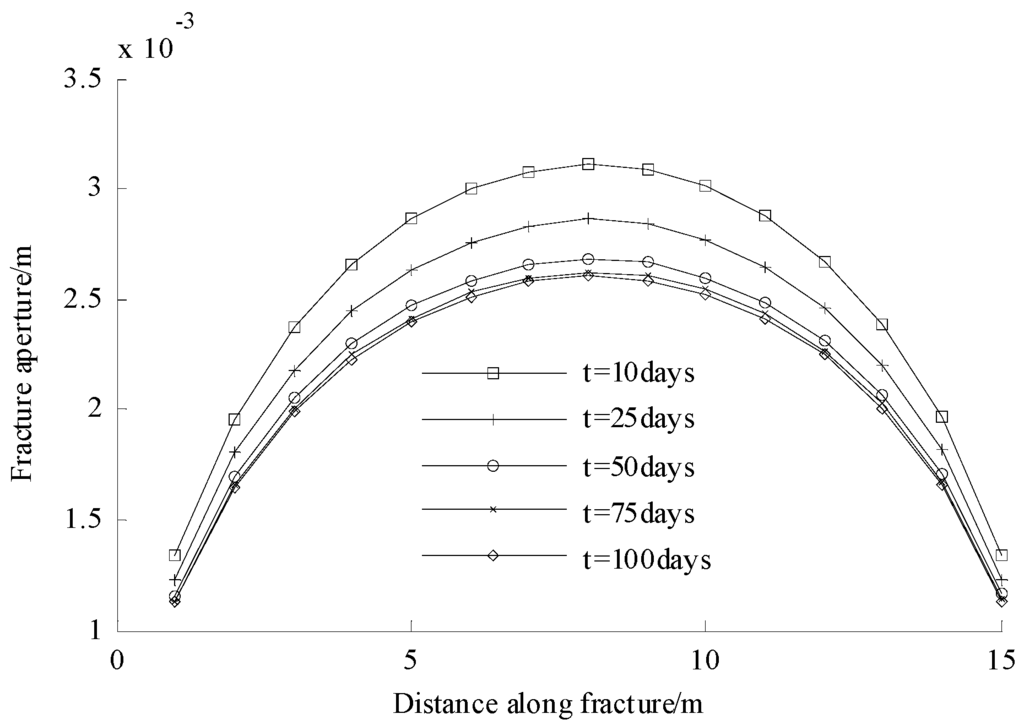
Figure 12. Fracture aperture distribution at different time.

The method is applied to another case, which consists of two intersecting fractures. The domain has an area of 10 m × 10 m. The results of FM-XFEM model and DFM-XFEM are also compared, as shown in Figure 13 and Figure 14. It can be shown from Figure 13 that the displacement fields along y direction are very close for two methods. The y displacements in the area above the fractures are much larger than that below the fractures. It can be shown from Figure 14 that the excess pore pressure distributions of two methods are identical. The pressure around the fracture is smaller than other area because of larger conductivities in the fractures.

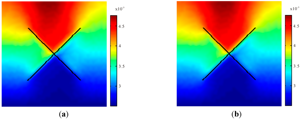
Figure 13. Displacement distribution (m) after 100 days. (a) FM-XFEM model; (b) DFM-XFEM model.

Figure 13. Displacement distribution (m) after 100 days. (a) FM-XFEM model; (b) DFM-XFEM model.

Figure 14. Excess pore pressure distribution (Pa) after 100 days. (a) FM-XFEM model; (b) DFM-XFEM model.

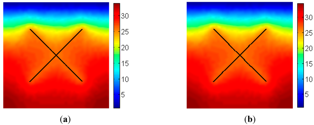
Figure 14. Excess pore pressure distribution (Pa) after 100 days. (a) FM-XFEM model; (b) DFM-XFEM model.

The water pressures at point (located at the right bottom) are shown in Figure 15a at varying mesh resolutions during 100 days. The plot is zoomed in for 10 days to clarify the discrepancies between the various curves as shown in Figure 15b. Also, the results of FM-XFEM model are shown in the figures. It can be shown that as the mesh resolutions become higher, the results converge to that of FM-XFEM. The differences between them are very small.

With regard to computational cost, the results are shown in Table 3. It can be shown that the computational cost of DFM-XFEM model is much less than that of FM-XFEM model. The results prove that the proposed method is better than FM-XFEM model.

Figure 15. Excess pore pressure at right bottom point. (a) 100 days; (b) 10 days.

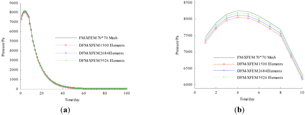
Figure 15. Excess pore pressure at right bottom point. (a) 100 days; (b) 10 days.

Table 3. Computational cost of models.

Models	Computational Time/s
FM-XFEM 50 × 50 Mesh	44.2
FM-XFEM 70 × 70 Mesh	101.3
DFM-XFEM 1500 Elements	11.4
DFM-XFEM 2684 Elements	22.1
DFM-XFEM 5926 Elements	50.1

Table 3. Computational cost of models.

Models	Computational Time/s
FM-XFEM 50 × 50 Mesh	44.2
FM-XFEM 70 × 70 Mesh	101.3
DFM-XFEM 1500 Elements	11.4
DFM-XFEM 2684 Elements	22.1
DFM-XFEM 5926 Elements	50.1

5. Conclusions

In this paper, the combination of discrete fracture model and extended finite element method is proposed to simulate fluid-solid coupling in fractured porous media. The discrete fracture model is able to capture fluid flow accurately without accessing cross flow between matrix and fracture. The extended finite element method is capable of solving solid deformation without mesh refinement around fractures tips. The model captures change of fracture aperture during the simulation. The results of numerical example show that the proposed method is well suited for simulating fluid-solid coupling in fractured porous media.

References

- Cottrell, M.; Hosseinpour, H.; Dershowitz, W. Rapid discrete fracture analysis of hydraulic fracture development in naturally fractured reservoirs. In Proceedings of the Unconventional Resources Technology Conference, Denver, CO, USA, 12–14 August 2013.
- Minkoff, S.E.; Stone, C.M.; Bryant, S.; Peszynska, M.; Wheeler, M.F. Coupled fluid flow and geomechanical deformation modeling. J. Petrol. Sci. Eng. 2003, 38, 37–56. [Google Scholar] [CrossRef]
- Boit, M.A. General Theory of Three-Dimensional Consolidation. J. Appl. Phys. 1941, 12, 155–164. [Google Scholar] [CrossRef]
- Terzaghi, V.K. Theoretical Soil Mechanics; John Wiley & Sons, Inc.: New York, NY, USA, 1943; pp. 2–30. [Google Scholar]
- Hou, G.; Wang, J.; Layton, A. Numerical methods for fluid-structure interaction—A review. Commun. Comput. Phys. 2012, 12, 337–377. [Google Scholar] [CrossRef]
- Moinfar, A.; Narr, W.; Hui, M.H.; Mallison, B.T.; Lee, S.H. Comparison of Discrete-Fracture and Dual-Permeability Models for Multiphase Flow in Naturally Fractured Reservoirs; SPE Reservoir Simulation Symposium: The Woodlands, TX, USA, 2011. [Google Scholar]
- Warren, J; Roor, P.J. The behavior of naturally fractured reservoirs. SPE J. 1963, 3, 245–255. [Google Scholar]
- Nie, R.S.; Meng, Y.F.; Jia, Y.L.; Zhang, F.X.; Yang, X.T.; Niu, X.N. Dual porosity and dual permeability modeling of horizontal well in naturally fractured reservoir. Transp. Porous Med. 2012, 92, 213–235. [Google Scholar] [CrossRef]
- Karimi-Fard, M.; Durlofsky, L.; Aziz, K. An efficient discrete-fracture model applicable for general-purpose reservoir simulators. SPE J. 2004, 9, 227–236. [Google Scholar] [CrossRef]
- Huang, Z.; Yao, J.; Wang, Y.; Tao, K. Numerical study on two-phase flow through fractured porous media. Sci. China Technol. Sci. 2011, 54, 2412–2420. [Google Scholar] [CrossRef]
- Lamb, A.R.; Gorman, G.J.; Elsworth, D. A fracture mapping and extended finite element scheme for coupled deformation and fluid flow in fractured porous media. Int. J. Numer. Meth. Eng. 2013, 37, 2916–2936. [Google Scholar] [CrossRef]
- Barenblatt, G.; Zheltov, I.P.; Kochina, I. Basic concepts in the theory of seepage of homogeneous liquids in fissured rocks [strata]. J. Appl. Math. 1960, 24, 1286–1303. [Google Scholar] [CrossRef]
- Belytschko, T.; Black, T. Elastic crack growth in finite elements with minimal remeshing. Int. J. Numer. Eng. 1999, 45, 601–620. [Google Scholar] [CrossRef]
- Stolarska, M.; Chopp, D.L.; Moës, N.; Belytschko, T. Modelling crack growth by level sets in the extended finite element method. Int. J. Numer. Eng. 2001, 51, 943–960. [Google Scholar] [CrossRef]
- Moes, N.; Gravouil, A.; Belytschko, T. Non-planar 3D crack growth by the extended finite element and level sets—Part I: Mechanical model. Int. J. Numer. Eng. 2002, 53, 2549–2568. [Google Scholar] [CrossRef]
- Gravouil, A.; Moes, N.; Belytschko, T. Non-planar 3D crack growth by the extended finite element and the level sets—Part II: Level set update. Int. J. Numer. Eng. 2002, 53, 2569–2586. [Google Scholar] [CrossRef]
- Gordeliy, E.; Peirce, A. Coupling schemes for modeling hydraulic fracture propagation using the XFEM. Comput. Method Appl. Mech. Eng. 2013, 253, 305–322. [Google Scholar] [CrossRef]
- Ghafouri, H.R.; Lewis, R.W. A finite element double porosity model for heterogeneous deformable porous media. Int. J. Numer. Meth. Eng. 1996, 20, 831–844. [Google Scholar] [CrossRef]
- Lewis, R.W.; Ghafouri, H.R. A novel finite element double porosity model for multiphase flow through deformable fractured porous media. Int. J. Numer. Meth. Eng. 1997, 21, 789–816. [Google Scholar] [CrossRef]
- Tran, N.H.; Ravoof, A. Coupled Fluid Flow through Discrete Fracture Network: A Novel Approach. Int. J. Math. Comput. Simul. 2007, 3, 295–299. [Google Scholar]
- Al-Khoury, R.; Sluys, L.J. A computational model for fracturing porous media. Int. J. Numer. Eng. 2006, 70, 423–444. [Google Scholar] [CrossRef]
- Viré, A.; Xiang, J.; Milthaler, F.; Farrell, P.E.; Piggott, M.D.; Latham, J.-P.; Pavlidis, D.; Pain, C.C. Modelling of fluid-solid interactions using an adaptive mesh fluid model coupled with a combined finite-discrete element model. Ocean Dyn. 2012, 62, 1487–1501. [Google Scholar] [CrossRef]
- Viré, A.; Xiang, J.; Pain, C.C. An immersed-shell method for modelling fluid-structure interactions. Phil. Trans. Royal Soc. A. 2015, 373, 20140085. [Google Scholar] [CrossRef] [PubMed]
© 2015 by the authors; licensee MDPI, Basel, Switzerland. This article is an open access article distributed under the terms and conditions of the Creative Commons Attribution license (http://creativecommons.org/licenses/by/4.0/).