Fast Computation of the Non-Central Chi Square PDF Outside the HDR Under a Requisite Precision Constraint

Abstract

Computation of the non-central chi square probability density function is encountered in diverse fields of applied statistics and engineering. The distribution is commonly computed as a Poisson mixture of central chi square densities, where the terms of the sum are computed starting with the integer nearest the non-centrality parameter. However, for computation of the values in either tail region these terms are not the most significant and starting with them results in an increased computational load without a corresponding increase in accuracy. The most significant terms are shown to be a function of both the non-centrality parameter, the degree of freedom and the point of evaluation. A computationally simple approximate solution to the location of the most significant terms as well as the exact solution based on a Newton–Raphson iteration is presented. A quadratic approximation of the interval of summation is also developed in order to meet a requisite number of significant digits of accuracy. Computationally efficient recursions are used over these improved intervals. The method provides a means of computing the non-central chi square probability density function to a requisite accuracy as a Poisson mixture over all domains of interest.

1. Introduction

Efficiently evaluating the non-central chi square probability density function (PDF) is of practical importance to a number of problems in applied statistics [1]. For instance, the ratio of two densities f(x)/p(x), where p(x) is a non-central chi square density, may be necessary in an importance sampling scheme or for hypothesis testing. The non-central chi square density [2], where λ is the non-centrality parameter and ν the degree of freedom, arises in the general case where x = e′Σ⁻¹e and $e~\mathrm{N}(\mu ,\sum )$, e ∈ R^ν, and Σ positive definite. It follows that $x~{\chi }_{\nu }^2(\mathrm{\lambda })$ where λ = µ′Σ⁻¹µ. The notation $e~\mathrm{N}(\mu ,\sum )$ implies that e has Gaussian distribution [3], $\mathrm{N}(\mu ,\sum )={(2\pi )}^{-\nu /2}{|\sum |}^{-1/2}\mathit{exp}(-\frac{1}{2}{(e-\mu )}^{\prime }{\sum }^{-1}(e-\mu ))$ and $x~{\chi }_{\nu }^2(\mathrm{\lambda })$ denotes that x is distributed as a non-central chi square with ν degrees of freedom and non-centrality parameter λ. For a non-central chi square variate E[x] = λ + ν, and Var[x] = 4λ + 2ν. The density at x can be represented [2] by

$$p(x;\nu ,\mathrm{\lambda })=1/2{(x/\mathrm{\lambda })}^{(\nu -2)/4}{I}_{\nu -2-1}(\sqrt{x\mathrm{\lambda }})\mathit{exp}(-(x+\mathrm{\lambda })/2)$$

where I_ν(x) is the modified Bessel function of order ν. However this representation is numerically problematic for large x or large λ. The asymptotic result $(x-(\mathrm{\lambda }+\nu ))/(\sqrt{2\nu +4\mathrm{\lambda }})~N(0,1)$ as λ or ν → ∞ can be useful, but is not a universal substitute for direct computation of p(x; ν, λ) even for relatively large λ. For this reason the discrete mixture representation

$$p(x;\nu ,\mathrm{\lambda })={\displaystyle \sum _{n=0}^{\infty }\frac{{(\mathrm{\lambda }/2)}^n}{n!}\mathit{exp}(-\mathrm{\lambda }/2)\cdot p(x;\nu +2n,0)=E_{n/\mathrm{\lambda }}[p(x;\nu +2n,0)]}$$

(1)

where it is recognized that the expectation is over the Poisson density [4] P(n|λ/2) = (λ/2)ⁿexp(−λ/2)/n! and

$$p(x;\nu ,0)=p_{\nu }(x)=\frac{x^{\nu /2-1}}{2^{\nu /2}\mathrm{\Gamma }(\nu /2)}\mathit{exp}(-x/2)$$

(2)

is the central chi square probability density function (PDF) [3] with ν degrees of freedom. The non-central chi square density at the point x is therefore the average of an infinite set of central chi square densities evaluated at x.

The goal of this article is to present a method to compute the value of the distribution function of a non-central chi square variate using the mixture representation and to do so with minimal computational effort to a specified accuracy in all domains of interest, including both the high density region (HDR) and the tail regions. In doing so, we will illuminate the often employed standard method and discuss the computational weaknesses that method has in the tails of the distribution. The cumulative density function (CDF) ${\displaystyle {\int }_0^{x}p(\alpha ;\nu ,\mathrm{\lambda })d\alpha }$ of the non central chi square has been addressed by [5] and the computational issues associated with the domains of evaluation have been addressed by a treatment dependent on the parameters, {x, ν, λ} [6].

2. Computation of p(x; ν, λ)

With the goal to compute p(x; ν, λ) to a specified accuracy for arbitrary x, λ and ν in a computationally efficient manner, start with the representation of the non-central chi-square density as a mixture of central chi-square densities:

$$p(x;\nu ,\mathrm{\lambda })={\displaystyle \sum _{n=0}^{\infty }f(x,n;\nu ,\mathrm{\lambda }),}$$

(3)

$$f(x,n;\nu ,\mathrm{\lambda })=\frac{{(\mathrm{\lambda }/2)}^n}{n!}\mathit{exp}(-\mathrm{\lambda }/2)\cdot \frac{x^{\nu /2+n-1}}{2^{\nu /2+n}\mathrm{\Gamma }(\nu /2+n)}\mathit{exp}(-x/2)$$

(4)

The sum is computed efficiently by ordering the terms to be summed according to their size, with the larger terms first and then for each of the terms to be summed exploiting the following recursions:

$$P(n+1|\mathrm{\lambda })=\frac{\mathrm{\lambda }}{2(n+1)}\cdot P(n|\mathrm{\lambda })p_{\nu +2n+2}(x)=\frac{x}{2n+\nu }\cdot p_{\nu +2n}(x),$$

thus ensuring that each term is computed in a computational efficient manner.

It is necessary to determine which terms maximally contribute to the sum and including these in the summation in order to meet the requisite accuracy. This domain of summation must provide for maximal computational efficiency for a given accuracy, or conversely minimal error for a pre-specified computational budget.

A popular approach, which is the basis of most algorithms in use, is to start the recursion at the mode of the Poisson density

$$n^P=\lfloor E[n|\mathrm{\lambda }]\rfloor =\lfloor \mathrm{\lambda }/2\rfloor$$

(5)

and proceed to sum in both directions until the relative accuracy is obtained. This approach is termed Algorithm 1.

Algorithm 1.

• n* = ⌊λ/2⌋, Equation (5), ϵ = 10−B

• Compute P (n*|λ), pν+2n*(x)

• Initialize: k = 1, ⌊p(x; ν, λ)⌋1 = P (n*|λ) · χ2ν+2n*

• 1. If n* − k ≥ 0 compute Rk = P (n* + k|λ) · pν+2n*+2k(x) + P (n* − k|λ) · pν+2n*−2k(x). Else if n* − k < 0 compute Rk = P (n* + k|λ) · pν+2n*+2k(x) via Equation (5).

2. Update ⌊p(x; ν, λ)⌋k = ⌊p(x; ν, λ)⌋k−1 + Rk−1

3. If Rk/⌊p(x; ν, λ)⌋k > ϵ then k = k + 1 and repeat.

4. Else ⌊p(x; ν, λ)⌋M1 = ⌊p(x; ν, λ)⌋k stop.

Algorithm 1.

• n* = ⌊λ/2⌋, Equation (5), ϵ = 10−B

• Compute P (n*|λ), pν+2n*(x)

• Initialize: k = 1, ⌊p(x; ν, λ)⌋1 = P (n*|λ) · χ2ν+2n*

• 1. If n* − k ≥ 0 compute Rk = P (n* + k|λ) · pν+2n*+2k(x) + P (n* − k|λ) · pν+2n*−2k(x). Else if n* − k < 0 compute Rk = P (n* + k|λ) · pν+2n*+2k(x) via Equation (5).

2. Update ⌊p(x; ν, λ)⌋k = ⌊p(x; ν, λ)⌋k−1 + Rk−1

3. If Rk/⌊p(x; ν, λ)⌋k > ϵ then k = k + 1 and repeat.

4. Else ⌊p(x; ν, λ)⌋M1 = ⌊p(x; ν, λ)⌋k stop.

This approach is nearly optimal for x in the high probability density region, however it is quite inefficient in the tail regions of the density. That is the mode, ⌊λ/2⌋ is quite distant from the maximally contributing terms of the summation in regions other than the high density region. For this reason, starting at ⌊λ/2⌋, as in Algorithm 1, wrongly focuses computation on terms that contribute little information to the numerical result. The optimal solution would start at the location of the peak of f(x, n; λ, ν). Determine this starting point by noting that as a function of n

$$f(x,n;\mathrm{\lambda },\nu )\propto \frac{{(x\mathrm{\lambda }/4)}^n}{\mathrm{\Gamma }(n+1)\mathrm{\Gamma }(v/2+n}.$$

(6)

Define

$$d_{n}lnf(n)=\frac{d}{dn}lnf(x,n;\mathrm{\lambda },\nu )=ln(x\mathrm{\lambda }/4)-\psi (n+1)-\psi (n+\nu /2)$$

and employ the series expansion for ψ(n + 1), the digamma function

$$\psi (n)=ln(n)+\frac{1}{2n}+{\displaystyle \sum _{k=1}^{\infty }\frac{B_{2k}}{2k\cdot n^{2k}}}$$

(7)

where B_k the k-th Bernoulli number, to yield

$$d_{n}lnf(n)=ln(x\mathrm{\lambda }/4)-ln((n+1)(n+\nu /2))+\frac{1/2}{n+\nu /2}+\frac{1/2}{n+1}+O(n^{-2}).$$

(8)

Define

$$n^{*}=argma{x}_{n}f(x,n/\nu ,\mathrm{\lambda })$$

(9)

and an approximate solution for the integer n ≥ 0 is

$$ln(x\mathrm{\lambda }/4)\approx ln((n+1)(n+\nu /2))$$

(10)

implying

$$n^{*}\approx max\left[0,\frac{1}{2}\left(\sqrt{x\mathrm{\lambda }+{\left(\frac{\nu }{2}+1\right)}^2-2\nu }-(\nu /2+1)\right)\right].$$

(11)

Notice that for x ≈ E[x|λ, ν] = λ + ν and λ > ν > 2 it follows that n^*(x = λ + ν) ≈ λ/2 = E[n|λ], the expected value of the Poisson mixture weights. The advantage of using Equation (11) is that it is both relatively simple, requiring only a square root operation on integers, and is accurate at locating the largest terms of the sum in both the high density region and the tail regions. As will be shown for domains outside of the high density region n^* is computationally efficiency relative to starting at ⌊λ/2⌋.

To determine argmax_nf(x, n|ν, λ) exactly, use a few Newton–Raphson iterations starting from Equation (11) as

$$n^{k+1}=n^k-Dg(n^k)I^{-1}(n^k),n^1=n^{*}\text{Equation}(11)$$

(12)

where

$$I(n)=\frac{d^2}{d{n}^2}lnf(x,n;\mathrm{\lambda },\nu )=-\psi (n+1)-\psi (n+\nu /2).$$

(13)

Since the solution is needed only to the nearest integer, a single iteration of Equation (12) is sufficient.

Algorithm 2.

• Compute n*(x, λ) by Equations (11) or (12), ϵ = 10−B.

• Compute P (n*|λ), pν+2n* (x).

• Initialize: k = 1, ⌊p(x; ν, λ)⌋1 = P (n*|λ) · pν+2n* (x)

• 1. If n* − k ≥ 0 compute Rk = P (n* + k|λ) · pν+2n*+2k(x) + P (n* − k|λ) · pν+2n*−2k(x). Else if n* − k < 0 compute Rk = P (n* + k|λ) · pν+2n*+2k(x) via Equation (5).

2. Update ⌊p(x; ν, λ)⌋k = ⌊p(x; ν, λ)⌋k−1 + Rk−1

3. If Rk/⌊p(x; ν, λ)⌋k > then k = k + 1 and repeat

4. Else ⌊p(x; ν, λ)⌋M2 = ⌊p(x; ν, λ)⌋k stop.

Algorithm 2.

• Compute n*(x, λ) by Equations (11) or (12), ϵ = 10−B.

• Compute P (n*|λ), pν+2n* (x).

• Initialize: k = 1, ⌊p(x; ν, λ)⌋1 = P (n*|λ) · pν+2n* (x)

• 1. If n* − k ≥ 0 compute Rk = P (n* + k|λ) · pν+2n*+2k(x) + P (n* − k|λ) · pν+2n*−2k(x). Else if n* − k < 0 compute Rk = P (n* + k|λ) · pν+2n*+2k(x) via Equation (5).

2. Update ⌊p(x; ν, λ)⌋k = ⌊p(x; ν, λ)⌋k−1 + Rk−1

3. If Rk/⌊p(x; ν, λ)⌋k > then k = k + 1 and repeat

4. Else ⌊p(x; ν, λ)⌋M2 = ⌊p(x; ν, λ)⌋k stop.

The result is computationally more efficient than Algorithm 1 for x outside the high probability region for a pre-specified accuracy. It does, however, require the initial computation of n^* via Equations (11) or (12) as well as retaining the need for computing the comparisons of Step 3 for each iteration. Employing the more accurate starting point of Equation (12) requires a Newton–Raphson iteration and thus the evaluation of the information scale, I(n). Since integer arithmetic is computationally insignificant relative to floating point arithmetic, the approach has merit for x outside the high probability region.

There is a further advantage to computing the information scale. The information scale I(n) gives an approximate measure of the number of terms required. This brings us to the last method presented: eliminate Step 3 from Algorithm 2 by simply approximating the domain of summation with a Laplace approximation [7] to f(x, n; λ, ν). The information scale is approximated with

$$I(n)=\frac{d^2}{d{n}^2}lnf(x,n;\mathrm{\lambda },\nu )=-\frac{1}{n+1}-\frac{1}{n+\nu /2}-\frac{1/2}{{(n+\nu /2)}^2}-\frac{1/2}{{(n+1)}^2}+O(n^{-3}).$$

These derivatives are approximations based on the truncated expansion of $ln(\mathrm{\Gamma }(n))=(n-1/2)ln(n)-n+ln(\sqrt{2\pi })+1/12n+O(n^{-3})$ [8], where O(n^p) is polynomial in n with maximal degree p.

The decimal place contribution of the term f(x, n; λ, ν) is

$$b_x(n)=lo{g}_{10}{\displaystyle \sum _{k=1}^{\infty }f(x,k;\mathrm{\lambda },\nu )-lo{g}_{10}f(x,n;\mathrm{\lambda },\nu )}$$

(14)

with a lower bound

$$b_x(n)>lo{g}_{10}\underset{k}{\max }\{f(x,k|\mathrm{\lambda },\nu )\}-lo{g}_{10}f(x,n;\mathrm{\lambda },\nu ).$$

(15)

We can attain accuracy to B decimal places by including in the sum terms for which

$$\{n:lnf(x,n;\mathrm{\lambda },\nu )>-B\cdot ln(10)+ma{x}_k\{lnf(x,k;\mathrm{\lambda },\nu )\left\}\right\}.$$

(16)

Therefore let

$$\begin{array}{c}{n}^{*}(x,\nu ,\mathrm{\lambda })=argma{x}_{n}lnf(x,n;\nu ,\mathrm{\lambda }),\text{Equation}(12)\\ D^{*}(B)=\{n:{|n-n^{*}|}^2<-B\cdot ln(10)I^{-1}(n^{*})/2\end{array}$$

(17)

and include in the summation only those terms within the set D^*(B). The advantage of computing the domain of summation a priori is that it obviates the need to compute the relative errors and the computation can be performed with a simple for loop. The terms can be summed from least to greatest, with terms near n = n^* + D^*(B) summed first in order to minimize accumulation errors. The disadvantage is that the set is larger than necessary, due to the approximation of Equation (15) as well as the Laplace approximation.

Algorithm 3.

• Compute : n*(x, λ) by Equation (12),

• $Lb=n^{*}-\sqrt{-2B\cdot ln(10)/I(n^{*})}$, $Ub=n^{*}+\sqrt{-2B\cdot ln(10)/I(n^{*})}$, Equation (17),

• Compute P (n|λ), pν+2n(x)

• Initialize: kl = ku = 1, ⌊p(x; ν, λ)⌋1 = P(n*|λ) · pν+2n(x)

• 1. Compute

– $R^{k_u}=P(n+k_u|\mathrm{\lambda })\cdot p_{\nu +2n+2k_u}(x)$,

– $R^{k_l}=P(n-k_l|\mathrm{\lambda })\cdot p_{\nu +2n-2k_l}(x)$ Equation (5).

2. Update ${\lfloor p(x;\nu ,\mathrm{\lambda })\rfloor }^k={\lfloor p(x;\nu ,\mathrm{\lambda })\rfloor }^{k-}{}^1+R^{k_l}+R^{k_u}$

3. – If ku < Ub then ku = ku + 1 repeat, else $R^{k_u}=0$.

– If kl > Lb then kl = kl − 1 repeat, else $R^{k_l}=0$,

– If ku = Ub & kl = Lb then ⌊p(x; ν, λ)⌋M3 = ⌊p(x; ν, λ)⌋k stop.

Algorithm 3.

• Compute : n*(x, λ) by Equation (12),

• $Lb=n^{*}-\sqrt{-2B\cdot ln(10)/I(n^{*})}$, $Ub=n^{*}+\sqrt{-2B\cdot ln(10)/I(n^{*})}$, Equation (17),

• Compute P (n|λ), pν+2n(x)

• Initialize: kl = ku = 1, ⌊p(x; ν, λ)⌋1 = P(n*|λ) · pν+2n(x)

• 1. Compute

– $R^{k_u}=P(n+k_u|\mathrm{\lambda })\cdot p_{\nu +2n+2k_u}(x)$,

– $R^{k_l}=P(n-k_l|\mathrm{\lambda })\cdot p_{\nu +2n-2k_l}(x)$ Equation (5).

2. Update ${\lfloor p(x;\nu ,\mathrm{\lambda })\rfloor }^k={\lfloor p(x;\nu ,\mathrm{\lambda })\rfloor }^{k-}{}^1+R^{k_l}+R^{k_u}$

3. – If ku < Ub then ku = ku + 1 repeat, else $R^{k_u}=0$.

– If kl > Lb then kl = kl − 1 repeat, else $R^{k_l}=0$,

– If ku = Ub & kl = Lb then ⌊p(x; ν, λ)⌋M3 = ⌊p(x; ν, λ)⌋k stop.

where it is understood that the comparison of step 3 need not be made, as a for loop can perform this function implicitly.

3. Results

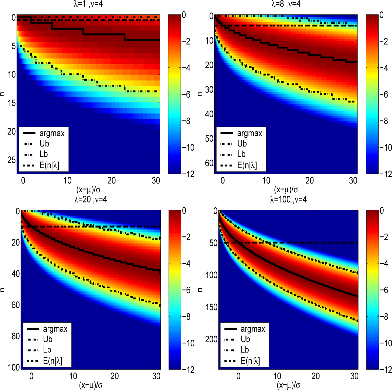
The three algorithms are compared to illustrate the importance of initialization of the algorithm by proper determination of n^*(x, ν, λ) in the computation of the non-central chi square PDF in the tail regions. First, Figure 1 depicts the normalized joint densities

$$r(x,n|\mathrm{\lambda },\nu )=lo{g}_{10}\frac{f(x,n;\mathrm{\lambda },\nu )}{ma{x}_n(x,n|\mathrm{\lambda },\nu )}$$

(18)

for ν = 4 and for diverse non-centrality parameters of λ =1, 8, 20 and 100. The initialization point, n^* for Algorithm 2 and Algorithm 3 are shown, as well as the conventional starting point ⌊λ/2⌋ of Algorithm 1. The difference between the actual maximum and ⌊λ/2⌋ is quite stark outside the HDR. Also shown are the Laplace approximate upper (Ub) and lower bounds (Lb) associated with B = 4 used for Algorithm 3.

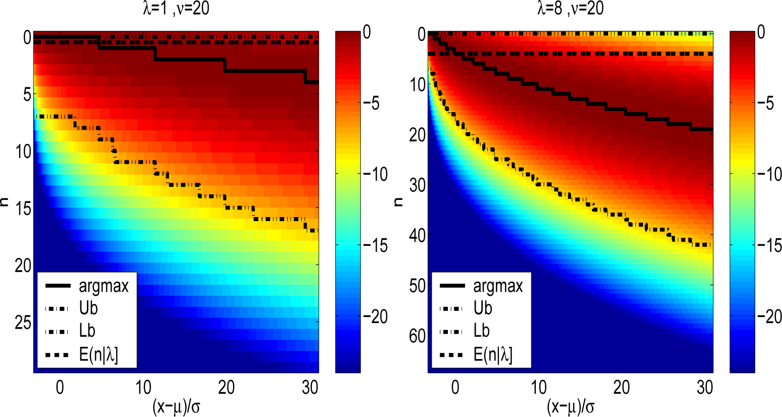
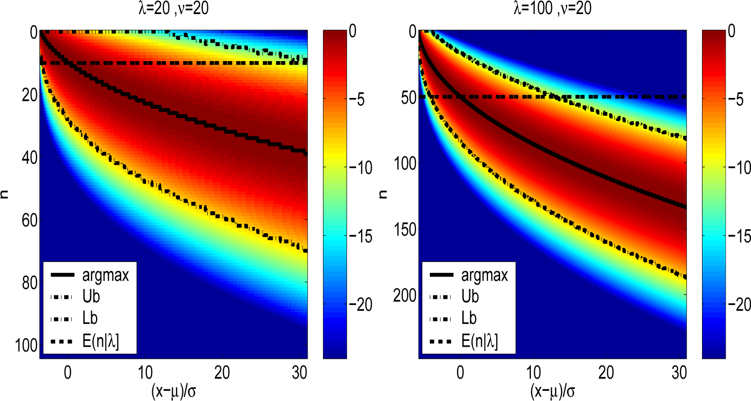
Figure 2 likewise depicts the normalized densities r(x, n|λ, ν) for a degree of freedom parameter value of ν = 20 and a range of non-centrality parameters λ =1, 8, 20 and 100. The increase in degree of freedom parameter relative to Figure 1 is shown to not significantly alter n^*(x, ν, λ). The upper and lower bounds of Algorithm 3 for B = 8 are shown. It is noted that for λ = 100 depicted in the lower right of Figures 1 and 2, the difference between n^* and ⌊λ/2⌋ in the lower tail of the distribution is also quite stark.

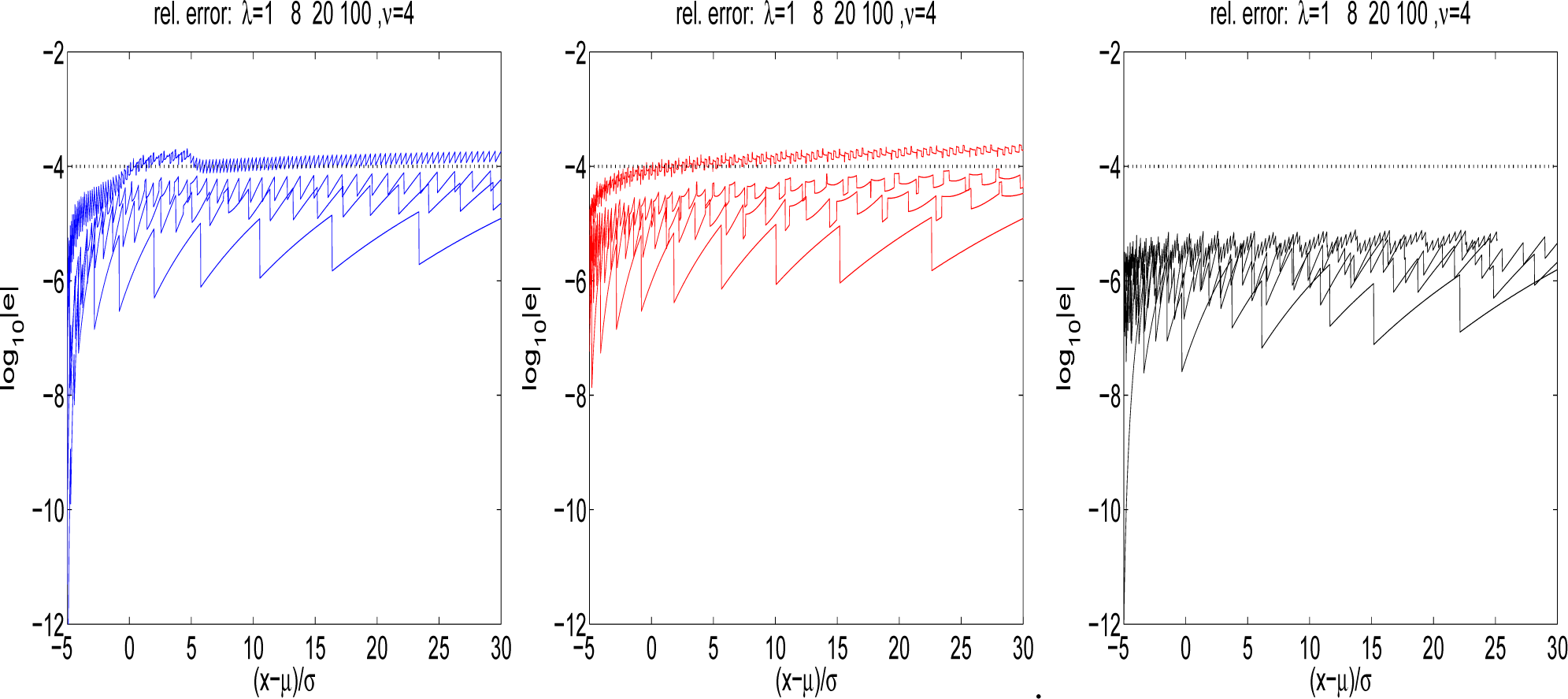
In order to demonstrate the performance of each of the three algorithms, they are each displayed relative to the value of the PDF computed from

$${\lfloor p(x;\nu ,\mathrm{\lambda })\rfloor }_{100}={\displaystyle \sum _{n\ge }^{|n-n^{*}|<100}\frac{{(\mathrm{\lambda }/2)}^n}{n!}\mathit{exp}(-\mathrm{\lambda }/2)}\cdot \frac{x^{\nu /2+n-1}}{2^{{}^{\nu /2+n}}\mathrm{\Gamma }(\nu /2+n)}\mathit{exp}(-x/2)$$

(19)

using the Algorithm 3 and summing least to greatest to obviate any accumulation errors. Define the relative errors of the 3 algorithms as follows

$$e_l(x)=\frac{{\lfloor p(x;\nu ,\mathrm{\lambda })\rfloor }_{M,l}}{{\lfloor p(x;\nu ,\mathrm{\lambda })\rfloor }_{100}},l=1,2,3$$

(20)

Figure 3 displays the relative errors for the three algorithms, with ϵ = 10⁻⁴. To the left and center are Algorithms 1 and 2 respectively, and the figure demonstrates the close proximity of each to a relative error of 10⁻⁴. To the right is Algorithm 3, and it can be seen that the use of the bounding approximation of Equation (15) implies that more terms are being included, such that an extra decimal place is attained across all non-centrality parameters shown.

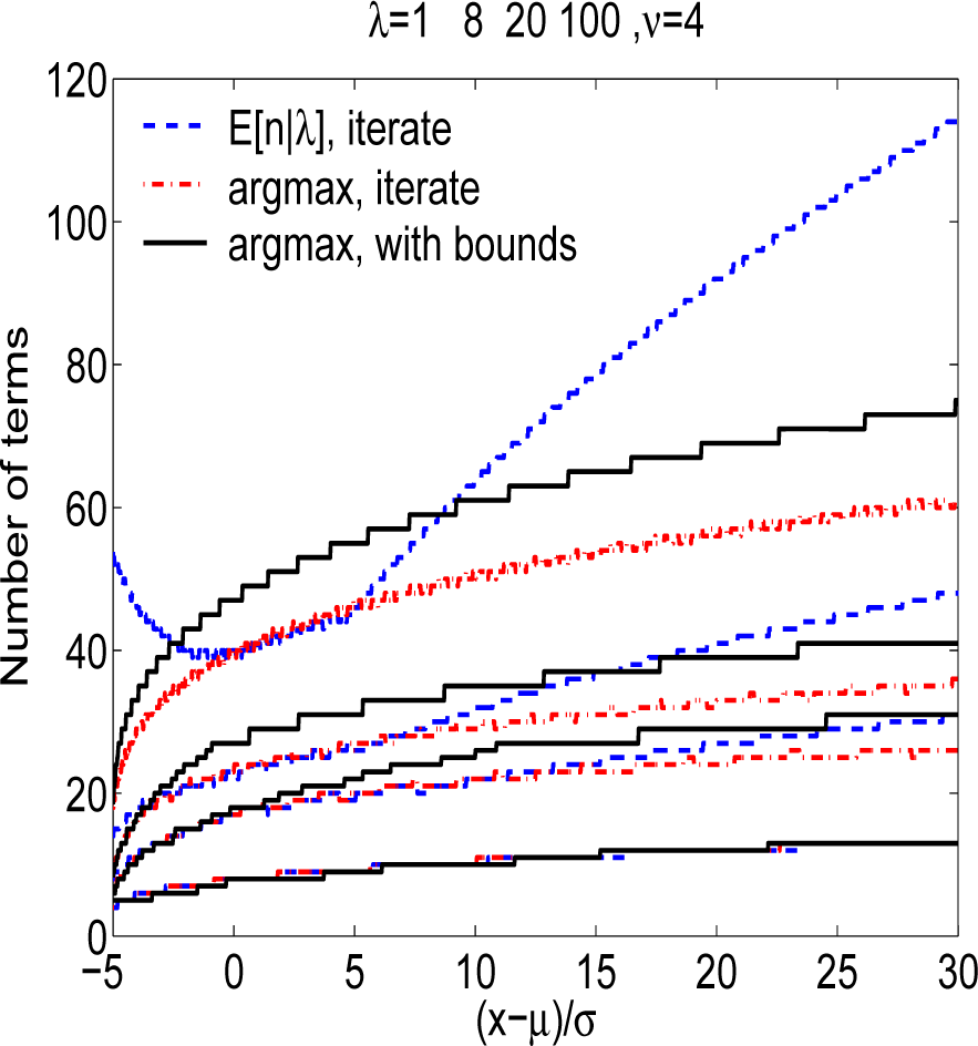
Figure 4 provides the number of terms necessary to attain the performance shown in Figure 3 for each of the algorithms. It is noted that only for λ = 100 in Algorithm 3 are the number of terms in excess of Algorithm 1 within the HDR. It is noteworthy that Algorithm 3 outperforms Algorithm 1 by over 2 × 40 floating point operations per evaluation in the tail region, since there are two additional floating point operation per iteration in Algorithm 1 that are not necessary in Algorithm 2.

4. Conclusions

The Poisson mixture representation of the non-central chi-square PDF is a useful and commonly employed means of computing the PDF at various domain values. The summation of terms is often initialized at the integer closest to half of the non-centrality parameter, the mode of the Poisson mixture weights ⌊λ/2⌋, and is efficient in the high probability density region (HDR). Outside of the HDR, the method is computationally inefficient, since the dominant terms in the sum are distant from the mode ⌊λ/2⌋. This shortcoming is addressed here by providing the maximally contributing terms in the sum regardless of the domain of evaluation. We do so in order to meet a requisite accuracy and computational load. The approach provides a simple means to retain the mixture representation for computation of the PDF outside of the HDR in a manner that is computationally reasonable. We present two methods to accomplish this task outside the HDR that provide a computation versus accuracy trade-off that is comparable within the HDR.