Engineering-Based Thermal CFD Simulations on Massive Parallel Systems

Abstract

The development of parallel Computational Fluid Dynamics (CFD) codes is a challenging task that entails efficient parallelization concepts and strategies in order to achieve good scalability values when running those codes on modern supercomputers with several thousands to millions of cores. In this paper, we present a hierarchical data structure for massive parallel computations that supports the coupling of a Navier–Stokes-based fluid flow code with the Boussinesq approximation in order to address complex thermal scenarios for energy-related assessments. The newly designed data structure is specifically designed with the idea of interactive data exploration and visualization during runtime of the simulation code; a major shortcoming of traditional high-performance computing (HPC) simulation codes. We further show and discuss speed-up values obtained on one of Germany’s top-ranked supercomputers with up to 140,000 processes and present simulation results for different engineering-based thermal problems.

1. Introduction

Due to ever-increasing advances in hardware, nowadays, high-performance computing (HPC) systems consist of several thousands to millions of cores, raising the necessity for sophisticated data structures and parallelization approaches in order to exploit the underlying computing power. The efficient ‘orchestration’ of hundreds of thousands of processes is one of the main challenges for high-fidelity applications to utilize massive parallel systems and, thus, leverage petaflop performance within multi-scale, multi-physics problems. In our approach, the focus was on coupling Computational Fluid Dynamics (CFD) simulations with thermal comfort assessment for complex engineering-based scenarios to be computed on modern HPC systems. Therefore, we have developed a hierarchical data structure that inherently supports distributed computing and combines state-of-the-art (numerical) solvers with efficient load-balancing techniques for fluid flow applications. This approach could be successfully tested on different HPC systems, including one of Germany’s three top-ranked supercomputers, up to a total of 140,000 processes solving a problem with close to one trillion (10¹²) unknowns.

Moreover, as the computed data have to be processed and analyzed in order to draw the necessary conclusions from the given problem statement, methods have to be devised to cope with the huge amount of data generated from a large run. Hence, the data structure is designed to handle interactive data exploration during runtime or to write a smaller, coarser data file for a subsequent offline post-processing. This issue is of major concern when it comes to analyzing HPC simulation data, as the problem sizes typically restrict data exploration and analysis. The work at hand provides a viable solution strategy.

There exist several state-of-the-art frameworks for problem solving environments (PSE), such as Chombo [1] or SCIRun [2], as well as open source CFD programs, such as OpenFOAM [3], which could have been used as foundations for algorithm development regarding an interactive data exploration. Furthermore, work has been done in the broad research area of in situ visualization (e.g., the state-of-the-art analysis by Rivi et al. [4]). The applications range from visualizing combustion problems (Yu et al. [5]) to general procedures and software solutions (Fabian et al. [6]) and extreme-scale scientific analysis (Bennett et al. [7]). From reviewing these platforms and concepts, the authors decided to develop a new data structure, allowing one to solve some of the mentioned shortcomings and to provide a flexible environment for further model implementations.

This paper, where parts are excerpts from Frisch [8] and rewritten in a condensed way in order to give a good overview over the strategies applied, describes ideas in order to create a computational fluid dynamics simulation program for indoor airflow purposes able to run on massive parallel systems, such as supercomputers and large clusters. In the following, the necessary mathematical concepts are introduced, based on the Navier–Stokes equations coupled to a temperature convection-diffusion equation by the Boussinesq approximation in order to model the thermal transport phenomena. The specifically tailored data structure, including the data exchange, is described, and efficient solving mechanisms based on a multi-grid-like solver for the pressure Poisson equation are introduced. A dedicated section treats the code validation and verification according to standard benchmarks, such as the Rayleigh–Bénard convection, before looking into engineering-based examples generated from everyday engineering needs using complex temperature boundary conditions, as well as a complex geometric setup.

2. Mathematical Modeling and Discretization

Starting from the conservation of mass, momentum and energy principles, the Navier–Stokes equations can be derived, which serve as a basis for the numerical modeling. A complete and extensive derivation, as well as the historical impact of the equations can be found in standard literature, such as [9–11]. The governing equations for an incompressible Newtonian fluid comprise three sets of equations. The first equation set, written in differential form, is called the continuity equation:

$$\nabla \cdot \overrightarrow{u}=0$$

(1)

where $\overrightarrow{u}$ describes the velocity of the fluid using u₁, u₂, u₃ as the three velocity components in the three spatial directions x₁, x₂, x₃, respectively This equation has to be satisfied at every time step all over the domain. The second set, called the momentum equations, can be written for every direction i ∈ {1,2,3} as:

$$\frac{\partial {\rho }_{\infty }{u}_i}{\partial t}+\nabla \cdot ({\rho }_{\infty }{u}_i\overrightarrow{u})=\nabla \cdot (\mu \nabla u_i)-\nabla \cdot (p{\overrightarrow{e}}_i)-{\rho }_{\infty }\cdot \beta \cdot (T-T_{\infty })g_i$$

(2)

where t represents the time, ρ_∞ the density of the fluid assumed constant over the complete domain and µ the dynamic viscosity p represents the pressure, β the thermal expansion coefficient of the fluid, T the temperature, T_∞ the temperature of the undisturbed fluid at rest and g_i the gravitational force in direction i. Here, ${\overrightarrow{e}}_i$ represents the unit vector in direction i.

The last term ρ_∞ · β · (T — T_∞)gi in the momentum conservation equation couples the effects of the temperature field to the momentum equations and is commonly known as the Boussinesq approximation. It is valid, if changes in the density occur only due to changes in the temperature, and can be described by a linear correlation between both variables. In other words, the density is everywhere assumed to be ρ_∞, and the last term ρ_∞ · β · (T − T_∞)g_i modifies the density due to buoyancy effects.

The last equation set describes the energy conservation equation in order to model the thermal heat transport. Using the generic convection-diffusion equation and adapting it to a heat transfer problem results in:

$$\frac{\partial T}{\partial t}+\nabla \cdot (T\overrightarrow{u})-\nabla \cdot (\alpha \nabla T)-\frac{q_{int}}{{\rho }_{\infty }\cdot c_p}=0$$

(3)

where α = k/(ρ_∞ · c_p) represents the heat diffusion coefficient, k the heat conduction coefficient, c_p describes the specific heat capacity at constant pressure and q_int the internal heat generation.

This equation is valid under the assumption that the variations of pressure are small enough in order to have no influence on the thermodynamic properties of the fluid. Following Lienhard and Lienhard [12], this assumption holds for most Newtonian fluids moving at moderate velocities slower than a third times the speed of sound, which is the case for indoor airflow scenarios. Furthermore, fluid properties, such as the thermal conductivity k or the dynamic viscosity µ, do not depend on changes in the temperature field. Moreover, the viscous dissipation of energy in the fluid must not heat up the fluid significantly.

Hence, under these conditions, Equation (3) models heat transport phenomena, such as convection and diffusion, along a given flow field $\overrightarrow{u}$. As the temperature field has again an influence on the flow field in Equation (2), a coupling strategy has to be applied.

Furthermore, by analyzing Equations (1)–(3), it can be seen that there is no independent equation for the pressure p. The momentum equations include the pressure gradient ∇p, whereas the incompressible continuity equation and the energy conservation equation do not contain p at all. Nevertheless, a solution for incompressible flows can be found by applying so-called pressure correction methods, proposed by Harlow and Welch [13] in their marker and cell method (MAC) for the solution of free surface flows or in the fractional step method (or projection method) introduced by Chorin [14]. The basic idea is to iterate between velocity and pressure fields, where the pressure field acts as a correction in order to fulfil the continuity equation for the velocity field. As Equation (2) only contains the pressure gradient, the absolute value of the pressure is not relevant, and thus, the pressure term p in the incompressible equations is often referred to as ‘working pressure’.

By applying the fractional step method and choosing an explicit Euler time discretization for the temporal derivative ∂/∂t, the momentum conservation equations in the direction i for an intermediate time step^⋆ can be written:

$${\rho }_{\infty }\cdot \frac{u_i^{\star }-u_i^n}{\mathrm{\Delta }t}=-\nabla \cdot ({\rho }_{\infty }{u}_i^n{\overrightarrow{u}}^n)+\nabla \cdot (\mu \nabla u_i^n)-{\rho }_{\infty }\cdot \beta \cdot (T-T_{\infty })g_i$$

(4)

by omitting the pressure gradient. Δt denotes the time step size, and the superscriptⁿ denotes the current time step n and the superscript^⋆ an intermediate time step between n and n + 1. The pressure term is now taken into account during a second step:

$${\rho }_{\infty }\cdot \frac{u_i^{n+1}-u_i^{\star }}{\mathrm{\Delta }t}=-\nabla \cdot (p^{n+1}{\overrightarrow{e}}_i)$$

(5)

While summing up the two Equations (4) and (5), it can be seen that Equation (2) results, where the velocity is treated explicitly (i.e., at time step n) and the pressure implicitly (i.e., at time step n + 1).

Using the divergence operator on Equation (5) leads to:

$${\rho }_{\infty }\cdot \frac{\nabla \cdot {\overrightarrow{u}}^{n+1}-\nabla \cdot {\overrightarrow{u}}^{\star }}{\mathrm{\Delta }t}=-\mathrm{\Delta }{p}^{n+1}$$

(6)

As the pressure term has to lead to a divergence-free velocity field at time step n + 1 with respect to the continuity Equation (1), the equation for determining the pressure at time step n+1 can be written as:

$$\mathrm{\Delta }{p}^{n+1}=\frac{{\rho }_{\infty }}{\mathrm{\Delta }t}\nabla \cdot {\overrightarrow{u}}^{\star }$$

(7)

representing a Poisson equation for the pressure, which has to be solved in every time step.

The temporal discretization can be enhanced using a second order explicit multi-level Adams–Bashforth method, introduced in detail by Schwarz [15], for example. A very detailed analysis of other time derivative approaches can be found in Ferziger [16]. Kim and Moin [17], for example, use a mixture of semi-implicit and explicit methods, where the convective terms in Equation (4) are discretized using a second order explicit Adams–Bashforth method. The viscous terms, however, are discretized using a semi-implicit Crank–Nicolson method, which eliminates some numerical stability problems. Choi and Moin [18] use a similar approach, but incorporate a predictor-corrector method.

Similar to a temporal discretization, a spatial discretization has to be introduced in order to describe and prepare the domain for a numerical simulation. Popular, well-established methods, such as the finite difference method (FDM), the finite volume method (FVM) or the finite element method (FEM), could be used. This work focuses on the finite volume and finite difference approach for discretizing the spatial domain. A good description of FDM and FVM methods in fluid mechanics can be found in Ferziger and Peric´ [10] or Hirsch [11], for example. In FDM, spatial derivatives are approximated using discretized notations of a certain order on a given grid. These derivatives can be used in equations expressed in differential form. In FVM, volume and surface integrals are computed by approximations of a certain order and used in equations expressed in an integral form. If finite volume methods are used on a regular Cartesian grid, it can be shown that the finite volumes degenerate into finite differences, which can be handled by a fast computational stencil, for example.

As an explicit time discretization method was chosen here, numerical stability issues have to be taken into account. Courant and Friedrichs [19] analyzed this problem in the 1920s and proposed using an upwind-difference for the convection term and central differences for the diffusive term. Peyret and Taylor [20] give a good overview on a detailed stability analysis for explicit finite difference methods.

3. Data Structure and Data Exchange

In order to store the relevant information required to simulate an airflow scenario, for example, a lean and efficient data structure has to be used. Furthermore, as the targeted hardware comprises supercomputers of all kinds, it is mandatory to design the data structure with a parallel implementation in mind, including consistent data synchronization mechanisms.

Hence, an efficient, parallel data structure is of utmost importance if computations on massive parallel systems shall be performed. The following sections will introduce the data structure and the necessary data synchronization and distribution mechanisms. Moreover, the basic idea of interactive data exploration enabled by the implemented data structure is introduced, highlighting the basic idea behind the chosen data structure concept. Furthermore, an efficient solving technique based on a multi-grid-like method is described, and scaling results from supercomputers will be discussed.

3.1. Data Structure

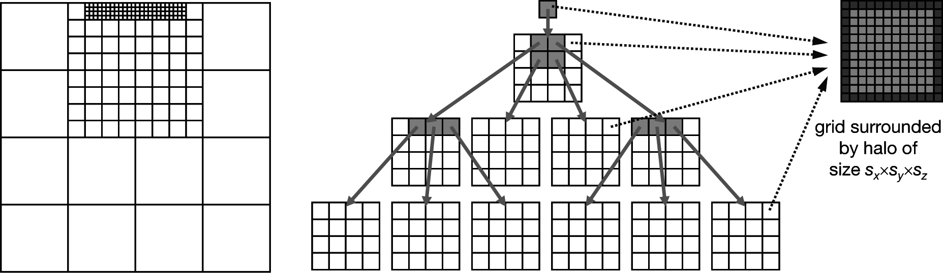
The data structure is based on non-overlapping, block-structured, hierarchical, orthogonal, regular grids. A logical, purely topological grid management (called ‘l-grids’) is responsible for all hierarchic information, such as parents and children relations, while data grids (called ‘d-grids’) contain the actual data arrays.

Figure 1 gives an overview of both data structure parts. In the middle part, the nested construction of the non-overlapping grids can be seen. A root l-grid, located per definition at depth zero, is refined by $r_x^t,r_y^t,r_z^t$ in the respective directions. The new resulting child l-grids can be refined again by $r_x^s,r_y^s,r_z^s$ until the desired depth d is reached. Currently, $r_i^t$ and $r_i^s$ can be chosen independently out of the interval [1, 7]. Furthermore, while creating the newly refined child l-grids, the coarse l-grid will be defined as their parent l-grid. Hence, each l-grid can only have one parent l-grid.

The second major part of the data structure is the d-grids (i.e., the data grids). Every d-grid stores the necessary variables, such as velocities, pressure or temperature values, in a matrix of cells. Thus, a cell is comparable to one finite volume or the control volume. It is surrounded by a halo of ghost cells necessary for the proper functioning of the structure. One of these d-grids can be seen on the right-hand side of Figure 1. It has a size of s_x, s_y, s_z (not counting the halo), which can be chosen arbitrarily with one constraint: in order to avoid non-conforming setups, s_i has to be divisible without any remainder by $r_i^s$ and by $r_i^t$. This restriction guarantees that coarse d-grid boundaries will always coincide with refined d-grid boundaries. Furthermore, each l-grid contains exactly one link to one d-grid.

Hence, due to the flexible structure of the logical grid management, complex, adaptive domain setups can be generated by combining regular blocks. By applying this type of data structure together with a finite volume approach for the spatial discretization, a few special points can be noted here.

One d-grid is constructed in such a way that it has an equidistant orthogonal spacing. In this case, it can be shown that the finite volume approach using the mid-point rule and linear interpolation degenerates into a finite difference approach. Thus, on one d-grid, a simple finite difference scheme, such as a six-point stencil in 3D, can be used. This allows a separation into two phases: a computation phase and a communication phase. In the computation phase, the finite difference approach in the form of a stencil, for example, is evaluated on every d-grid. In the communication phase, a halo update is performed filling the ghost cells with neighboring values in order to apply a Schwarz method [21]. Usually, a communication phase is only necessary for a computation running on a distributed system, but for this structure, it is required even in serial cases.

One difference between this data structure and data structures used by other codes is the retaining of the parent l-grids after a refinement into sub-grids. This generates an additional amount of data, which has to be stored, but this strategy poses great advantages in working with adaptive grids and during visualization post-processing, which will be presented in Section 3.4 after the data exchange and solving techniques are properly introduced.

3.2. Data Exchange

As the d-grids do not know anything about their neighbors and can purely compute on their local values, all other information, such as neighboring and parental relations, have to be provided by the logical grid management structure. Hence, the logical grid management has to take care of flux conservation across boundaries of d-grids, especially in the case of adaptive refinements, such as depicted in Figure 1. Therefore, complex data exchange mechanisms have to be provided by the logical grid management framework in order to guarantee data consistency and integrity.

In order to uniquely identify grids distributed over different processes, a UID (unique grid identifier) was introduced, composed out of a 64-bit integer. The first 32 bits contain the rank of the process on which the grid resides. The last 32 bits are used as a tag and encode in 22 bits the grid ID (GID), as well as in nine bits the location of this grid in the corresponding parent grid. Details of the tag encoding can be found in [8]. This coding proves quite convenient while using the message passing interface (MPI) libraries for communication, as the rank and tag can be immediately used for communication purposes.

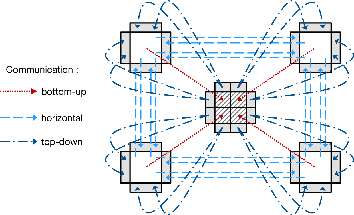
In [22], the basic communication routines were introduced, and they are displayed in Figure 2. The parallelization, of logical grids to different processes, where the data grids can use their internal finite difference stencil and the ghost halos are exchanged at specific times.

The distribution to different processes is managed by a special dedicated process called the neighborhood server. It is described in detail in [8]. The basic idea is to have one dedicated server keeping track of the logical structure for all grids (without having knowledge of the data content) and to organize the distribution to different processes by a space-filling curve in order to keep neighboring grids as close together as possible. Performance measurements showed very good results in terms of grid-to-grid communication for the distribution.

In order to ensure a consistent data exchange, a certain order has to be maintained during the exchange phase. In a serial computation, a synchronization is implicitly given by the ordering of the lines of code, and, obviously, it is necessary that data have to be available in the ghost halo before the stencil can use them for computing updated values or further exchanging them with neighboring grids.

In the case of a parallel computation, the same prerequisites have to be fulfilled: data must have been exchanged completely in all ghost halos of one d-grid, before a computation can start. Thus, synchronization mechanisms have to be implemented, preventing a computation before all necessary data have been exchanged. In a distributed parallel computation, synchronization is performed due to the existence of messages, i.e., by explicit message exchanges between different processes.

Generally, the communication is distributed into three phases: in the first stage, a bottom-up phase aggregates data from child grids and stores them in their corresponding parent grid. As soon as a parent receives data from all of its child grids, it aggregates its own data and sends them to its parent, and so on, until the root grid is updated. As the data are moving from the bottom to the top, the phase is dubbed bottom-up. In the next phase, direct neighbors exchange their values and store them in the corresponding ghost halos of their neighbors. In the case of an adaptive grid setup, it is important to do this data exchange only after the first phase finishes, as otherwise, inconsistent data storage could arise. In the last step, all ghost halos that did not receive any data from neighboring grids (thus, there was no neighboring grid at the same level) are filled with data from their corresponding parent grid. Once this step is finished, a complete and correct data exchange is done, and the computation step can work on the exchanged data.

From a technical point of view, all communications are managed by the MPI library, and data synchronization is achieved by combining blocking and non-blocking communication calls at the right places in the code.

In order to evaluate the behavior of the exchange mechanisms using large setups, tests were performed on different machines for different depths of the hierarchical data structure. Figure 3 shows the times for one ghost halo exchange of the complete grid structure. The measurements were performed on three testing systems: Shaheen ( http://www.hpc.kaust.edu.sa), a 16-rack IBM Blue Gene/P supercomputer installed at King Abdullah University of Science and Technology (KAUST) in the Kingdom of Saudi Arabia, the MAC Cluster ( http://www.mac.tum.de), a heterogeneous research cluster installed by the Munich Centre of Advanced Computing at Technische Universität München in Germany, and SuperMUC ( http://www.lrz.de/services/compute/supermuc/systemdescription), a 155,656 processor core large IBM System iDataPlex supercomputer installed at the Leibniz Supercomputing Centre (LRZ) in Garching, Germany.

All curves show a tendency of decreased exchange time with increased amount of processes. The curves for depth eight describe a uniformly-refined domain using approximately 78.5 billion cells, and more than 707 billion variables are exchanged across more than 140,000 processes on SuperMUC. Hence, the data structure in its current form is extremely flexible and is well suited for massive parallel machines.

3.3. Multi-Grid-Like Solver for the Pressure Poisson Equation

Geometric multi-grid solvers were introduced in the 1970s by Brandt [23] as multi-level methods. The general idea is based on the fact that many iterative methods, such as Jacobi or Gauss–Seidel, have a smoothing effect on the error if they are applied to elliptic problems (cf. Trottenberg et al. [24]), where high-frequency components of the error will be damped much more than low-frequency components. Hence, using only a smoothing method requires a long time to reduce the overall error below a certain tolerance. Fortunately, it can be shown that by approximating a quantity to a coarser grid, the smooth behavior will become oscillatory again, and the smoothing strategy can be reapplied. As soon as the coarsest grid is small enough, it can be solved by a direct solver, for example. Once a solution is available, the error correction can be forwarded from coarse grid to a fine grid, until the finest grid is updated.

The passing from a fine to a coarse grid is called restriction and from a coarse to a fine grid prolongation. Different restriction and prolongation operators can be found in Briggs et al. [25], for example.

By comparing the data flows of restriction and prolongation operators to the previously described phases of the communication, many similarities can be seen. Hence, a cell-centered, multi-grid like solver was implemented using the already existing communication routines. Different smoothing strategies were analyzed and compared, in order to find suitable settings, working for the intended types of problems. Details can be found in [26], for example.

As the first testing example, a Laplacian equation was used, as this equation is similar to the pressure Poisson equation, which has to be solved at every time step in order to account for the pressure correction and guarantees the validity of the continuity equation. The Laplacian problem:

$$\mathrm{\Delta }p(x,y,z)=\frac{{\partial }^{2}p(x,y,z)}{\partial x^2}+\frac{{\partial }^{2}p(x,y,z)}{\partial y^2}+\frac{{\partial }^{2}p(x,y,z)}{\partial z^2}=0$$

(8)

is defined on a 1 × 1 × 1 m cubic domain, where fixed Dirichlet boundary conditions were applied on the east and west side according to:

$$p(0,y,z)=p(1,y,z)=1\forall y,z$$

(9)

whereas all other sides were set to p = 0. This equation describes a pure diffusion process and could be used as well for modeling a stationary temperature diffusion problem without any convective influences or internal loads.

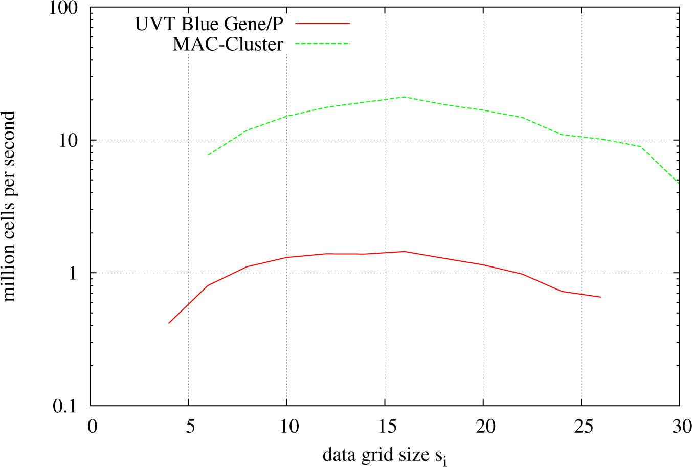
Before doing a large-scale analysis of the code’s performance for the Laplacian problem on a supercomputer, such as SuperMUC, small-scale analyses were performed in order to determine an optimal data grid size for this type of problem and the given hardware. As mentioned in the section describing the data structure, the overall domain discretization is dependent on the chosen grid refinement $r_i^t$ and $r_i^s$, but also on the chosen data grid size s_i. In order to assess the influence of the data grid size on the performance, the Laplacian problem was solved for different data grid sizes on a Blue Gene/P system of Universitatea de Vest din Timişoara (UVT) in Romania and on the TUM MAC Cluster using 256 processes.

Figure 4 plots the number of solved cells per second (in millions) over the data grid size. Two facts can be observed from the resulting plot: there exists somewhere an optimal setting for the data grid size, lying around 16³ cells per data grid. Moreover, it can be seen that the Blue Gene/P is around an order of magnitude slower than the MAC Cluster. This can be well explained by the hardware differences of the systems. While the Blue Gene/P uses PowerPC processors with a clock speed of 850 MHz, the MAC Cluster and SuperMUC use Sandy-Bridge processors with 2.7 GHz. Furthermore, measurements of the network interconnect showed a speed difference of a factor six in favor of the MAC Cluster. Additionally, other effects, such as different cache sizes or memory bandwidths, have to be taken into consideration. Hence, a factor of 10 can be justified from a hardware-based point of view.

Table 1. Domain sizes for measurements using a recursive bisection and a data grid size of 16³.

Depth	Number of l-Grids	Number of Cells	Total Required Memory (GB)
5	37,449	0.15×109	54.7
6	299,593	1.23×109	437.6
7	2,396,745	9.82×109	3500.9
8	19,173,961	78.54×109	28,007.2

shows the number of l-grids and the total number of cells in the domain, if a uniform grid refinement up to a certain depth and a data grid size of 16³ is applied. Furthermore, the total amount of required memory is listed in the last column of the table. Thus, a uniform refinement up to depth eight will generate a total of around 20 million l-grids and more than 78.5 billion cells, requiring 28 TB of main memory for storing all relevant data. Thus, on SuperMUC with around 1.5 GB of memory per core available to applications, a problem using Level 8 requires at least 20,000 processes to run.

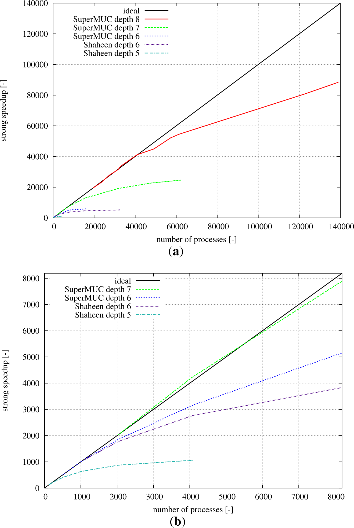
Figure 5 shows the strong speed-up results measured on SuperMUC and on Shaheen. While Figure 5a gives a complete overview of the complete range of scaling up to 140,000 processes on SuperMUC, Figure 5b zooms into the area of up to 8192 cores. On SuperMUC, depth eight with 78.5 billion cells can still show a parallel efficiency of 64% at 140,000 computing cores. Similar results can be seen for depth seven at 32,000 processes. At some point, the curves start to level off, and the parallel efficiency decreases. In a strong speed-up case, this is well known, as the communication overhead increases with a constant amount of computations. Hence, knowing the performance curves for a given hardware architecture, the amount of processes and refinement levels can be chosen in a way to maximize the throughput for a specific problem size.

Further measurements on adaptive grid setups (i.e., where not all of the levels are refined uniformly) were performed and showed very similar behavior and results regarding time to solution and ghost cell exchange times. The interested reader is referred to [8] for further details.

3.4. Visualization Strategies

In order to cope with the tremendous data advent generated by CFD simulations, special consideration has to be given to data visualization and interpretation.

Standard methods dump the generated data to hard disks to perform an offline post-processing. In the case of the above-mentioned large example for depth eight computed on SuperMUC having a memory footprint of over 28 terabytes, such a ‘standard’ solution is unfeasible.

Hence, new solutions have to be used in order to tackle this ‘Big Data’ problem. One goal during the design phase of the given data structure was to provide interactive data exploration capabilities. The general and technical context is explained in detail in Mundani et al. [27] and will be briefly introduced here.

The main idea of the interactive data exploration is based on a constant bandwidth approach, where the data density is kept constant. Hence, if only a small region in the computational domain is currently of interest, only this part is visualized at full resolution. If a larger domain should be regarded, the bounding box around the window of interest is increased, while taking only every second data point into consideration and, thus, keeping the data density constant. This window of interest can be moved around in order to visualize different regions of the domain and, hence, yields to the name ‘sliding window approach’. If the complete domain should be visualized, only a coarse representation is returned, giving a general idea of the flow patterns, but omitting details from the finer grids.

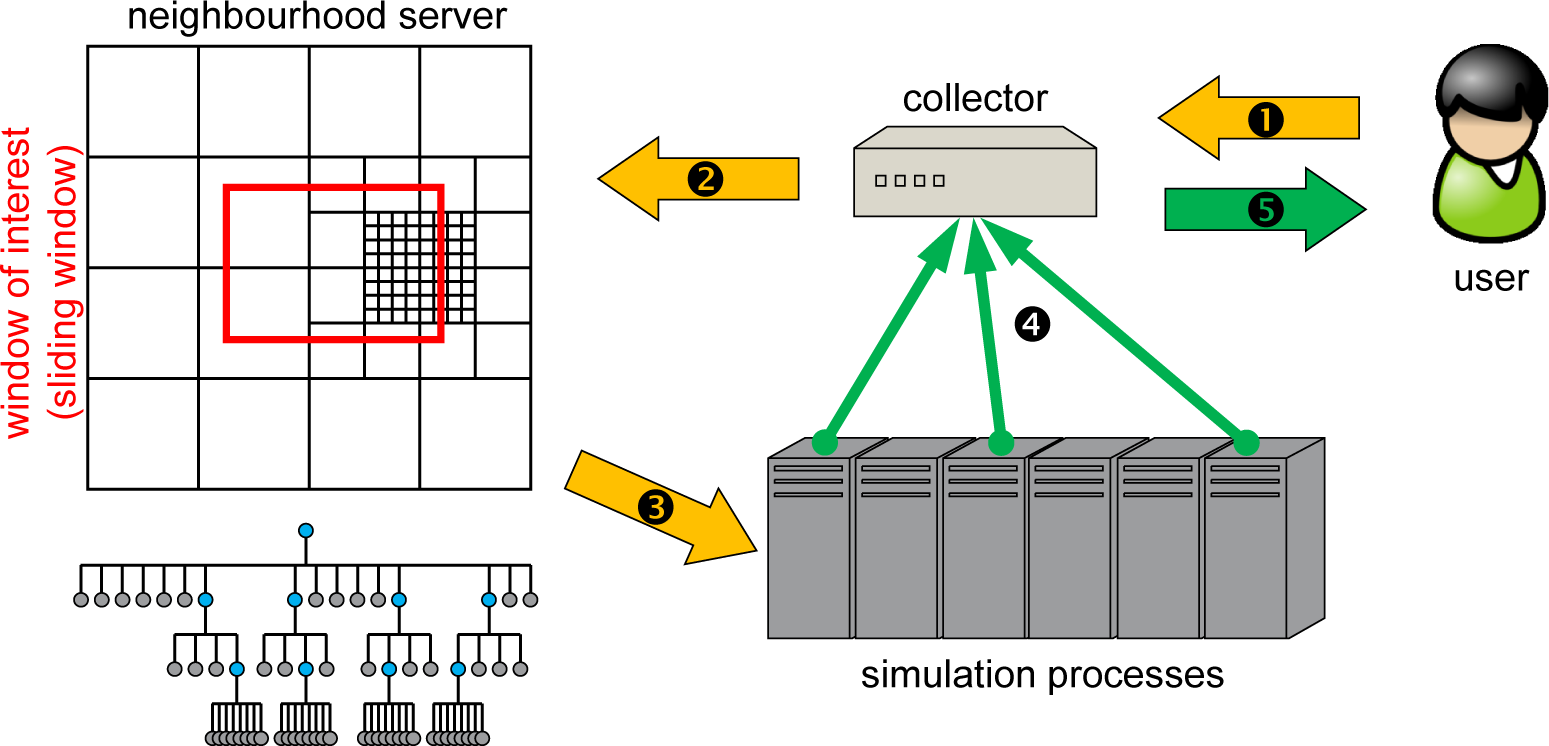
Technically, the process is fully integrated into the data structure itself and requires fully populated data grids on all levels, which are generated automatically during the synchronization process. Figure 6 depicts the schematic process. The user contacts a collector server, requests visualization information and sets a sliding window bounding box. The collector contacts the neighborhood server(s) and orders a visualization of certain areas. As the neighborhood server knows the topological allocation of grids, it orders (only) the involved computing processes to send visualization data directly to the collector process, which receives the single parts, compresses them in a data stream and passes them on to the user. The communication between collector and user is based on pure TCP/IP socket communication and does not require any MPI involvement. Hence, a user can connect to the collector from any computer at any time, visualize data and disconnect. The introduced data structure poses multiple advantages. Due to the neighborhood server design, only processes where data grids are touched by the sliding window will be contacted for delivering results to the collector process. Hence, it is not necessary to engage in an all-to-all communication. Furthermore, as the communication structures provide already aggregated data at different levels in the data structure, the data can be used immediately at every level for visualization and do not require any post-processing in order to generate coarsened data.

In case a supercomputing center does not allow interactive connections to the machines running the code, the same procedures can be used to dump data only partially to disk for a subsequent post-processing analysis, exactly as in the case of the interactive visualization.

In the next stage, the same data structure could be used to enable computational steering capabilities, where boundary conditions, fluid properties or geometry definitions could be changed during runtime, and an effect could be instantaneously observed in the simulation results (see Mulder et al. [28]).

4. Verification and Validation

Validations and verifications were performed for different standard benchmarks and test examples, such as the lid-driven cavity example in 2D and 3D, a pure channel flow in 2D and 3D and a von Kármán vortex street according to the Schäfer–Turek benchmark described in the DFG (Deutsche Forschungsgemeinschaft) priority research program ‘Flow Simulation on High-Performance Computers’ [29]. These benchmarks were used to test the behavior for isothermal settings, i.e., without a thermal coupling using the Boussinesq approximation, and will not be described here. The interested reader is referred to [8] for further details and results.

In order to test the thermal coupling, natural convection scenarios due to heated side-walls and due to heated floors and ceilings were analyzed. Although these two configurations seem quite similar, the flow patterns are completely different.

4.1. Test Case: Heated Side-Walls

As the first case, heated side-walls are analyzed, where the fluid flow is purely driven by natural convection phenomena. The fluid properties are described by the Prandtl number Pr, indicating the ratio of momentum diffusivity to thermal diffusivity, and the Rayleigh number Ra, describing if the heat transfer process is dominated by conduction or convection effects. All benchmark examples use a Prandtl number of Pr = 0.71 (properties of air), whereas the Rayleigh number is varied in order to model different fluid viscosities. The left-hand wall of the square cavity is heated, whereas the right-hand wall of the cavity is cooled and modeled by fixed Dirichlet boundary conditions. The top and bottom walls are perfectly isolated and regarded as adiabatic (i.e., using homogeneous Neumann boundary conditions). The gravitation vector is pointing downwards and, thus, is parallel to the heated and cooled walls.

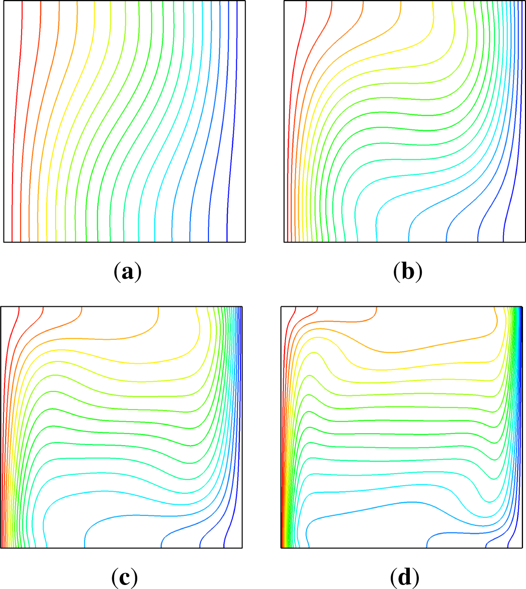
Figure 7 shows the isothermal profiles indicating the temperature distribution in the cavity for different Rayleigh numbers on a 256² domain resolution. Comparisons to results published by De Vahl Davis [30], Phillips [31], Eggels et al. [32] or van Treeck [33] are in excellent agreement with the simulated results.

In order to obtain a better quantification, the Nusselt number Nu for the hot wall at x = 0 can be calculated for this benchmark according to Eggels et al. [32] by:

$${Nu:=-\frac{1}{\mathrm{\Delta }T}{\displaystyle {\int }_0^{l_y}\frac{\partial T(x,y)}{\partial x}}|}_{0,y}\mathrm{d}y$$

(10)

where a higher order approximation following Phillips [31] is used for the temperature gradient discretization:

$$\frac{\partial T(x,y)}{\partial x}{|}_{0,y}\frac{-3T(0,y)+4T(\mathrm{\Delta }x,y)-T(2\mathrm{\Delta }x,y)}{2\mathrm{\Delta }x}$$

(11)

where Δx is the cell width used for the current discretization. The Nusselt number characterizes the ratio of convective heat transfer to conductive heat transfer.

Table 2. Comparison of simulated Nusselt numbers at the hot wall (x = 0) to results published in the literature.

Ra	Nusim (N=256)	[30]	[34]	[35]
103	1.11772	1.117	—	1.1170
104	2.24466	2.238	—	2.2435
105	4.51976	4.509	—	4.5168
106	8.78860	8.817	8.8250	8.8239
107	15.9137	—	16.5230	16.5571

shows the results of the simulation and reference values from the literature. When comparing the simulated results to the values published by De Vahl Davis [30] up to Ra = 10⁶, the errors for the domain discretization of 256² range between 0.06% and 0.32%, which shows great agreement with the given reference solutions.

For higher Rayleigh numbers of 10⁷, however, an error of around 3.7% for a discretization of 256² is relatively high. This is probably due to the fact that the current simulation kernel uses only a standard central difference approximation for the convective terms in the momentum equations. Here, a donor-cell scheme, as described by Hirt et al. [36], can remedy the situation by mixing central differences with upwind differences for the convective terms.

By normalizing the velocity $u_y^{*}$ in the y-direction, as defined according to Eggels et al. [32]:

$$u_y^{*}=u_y\cdot {\left(\Vert \overrightarrow{g}\Vert \cdot \beta \cdot \mathrm{\Delta }T\cdot l_y\right)}^{-1/2}$$

(12)

the analysis can be compared to the literature results. l_y represents here the height of the cavity.

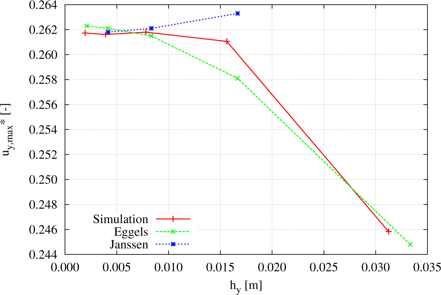
Figure 8 shows the influence of refining the grid discretization. The x-axis displays the width of one simulation cell, while keeping the total length constant. Hence, there exists a quadratic convergence characteristic towards finer mesh widths. Furthermore, it can be seen that different simulation models indicated in the literature have different characteristics, but converge towards a similar value.

While measuring and comparing the normalized maximum velocity $u_{y,sim}^{*}=0.2616$ for Ra = 10⁶ and a discretization of 256² to the references $u_{y,ref}^{*}=0.2618$ given by Janssen [37] for a discretization of 240², the error lies in the area of 0.07% and indicates good agreement of the simulated values using the above-described code and data structure.

4.2. Test Case: Rayleigh–Bénard Convection

In the second example, the heated and cooled surfaces are not side-walls, but the floor and the ceiling. As an infinitely long example should be regarded, the side-walls are modeled as periodic boundary conditions, connecting the left-hand side and right-hand side walls. The gravitational force is pointing downwards; thus, the temperature gradient is acting now against the gravitational force, and the resulting flow pattern is called Rayleigh–Bénard convection, analyzed by Bénard in [38] and by Lord John William Strutt, Third Baron Rayleigh.

The fundamental difference between the previous benchmark using heated side-walls and the Rayleigh–Bénard convection is that a critical threshold of the Rayleigh number has to be reached before the fluid is set in motion by convection phenomena. If the domain is sufficiently long and wide, the critical Rayleigh number is according to Pellew and Southwell [39]:

$$R{a}_{crit}\approx 1707.8$$

(13)

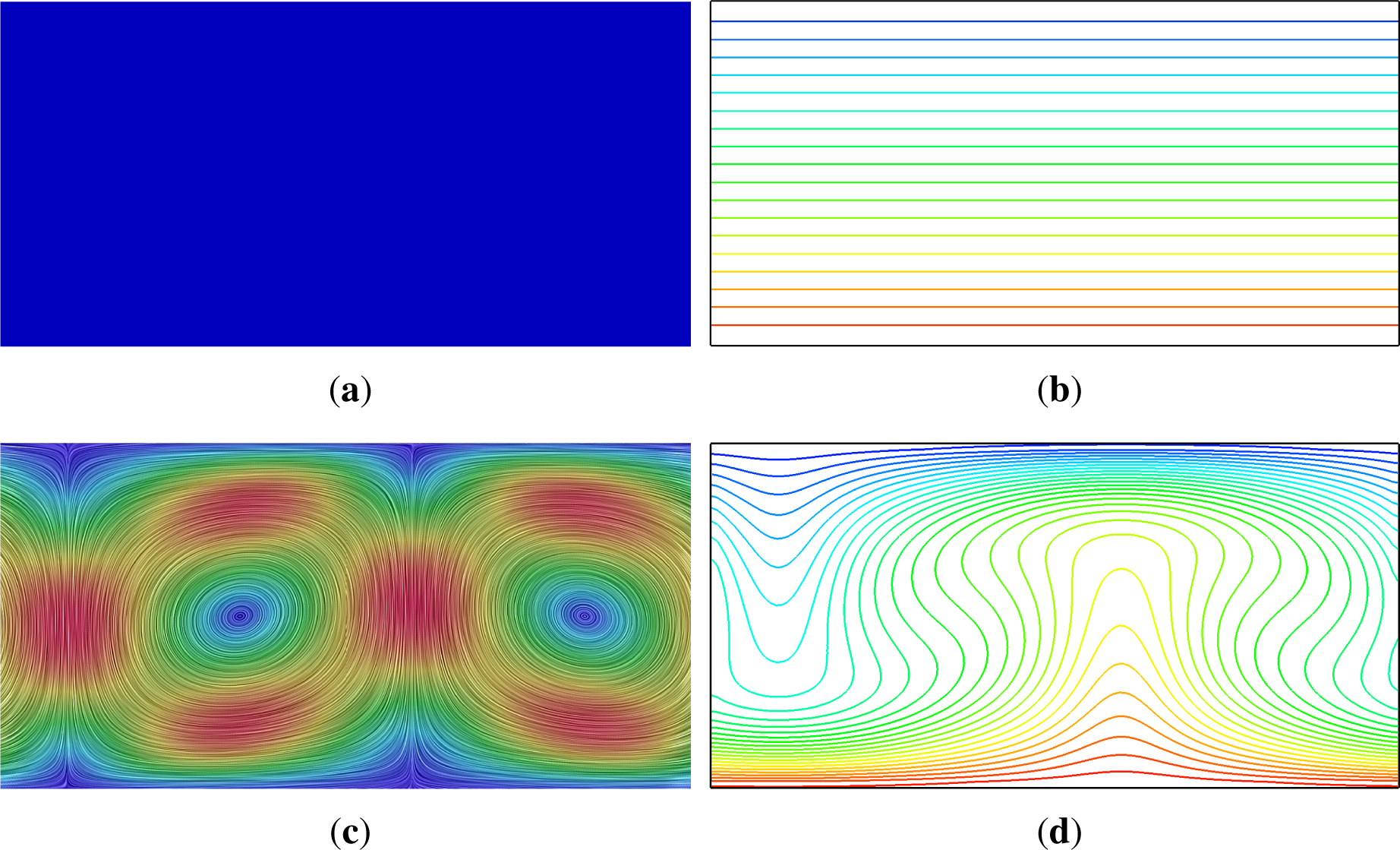
In Figure 9, two typical flow profiles can be seen. In the case of Ra = 1100, a sub-critical case, a thermal stratification can be observed. Hence, the fluid is at rest, and the heat is transported by conduction through the medium from the warm to the cold side. In case of Ra = 8000, a super-critical case, Rayleigh–Bénard convection cells are formed, and the isotherms show hot plumes rising up, getting cooled and descending to the bottom again.

In order to determine the critical Rayleigh number using the simulation results, the kinetic energy in the system is evaluated for several simulations using different Rayleigh numbers. The kinetic energy is computed by E_kin = 1/2 · m · v², where m represents the mass and v the velocity of the system. By expressing the mass m by the density ρ and the volume V, the kinetic energy can be rewritten as E_kin = 1/2 · ρ · V · v². By evaluating the kinetic energy of every cell and summing up all of the contributions, the total kinetic energy E_kin of the system at the time step t can be computed by:

$$E_{kin}(t)=\frac{1}{2}\cdot {\displaystyle \sum _{i,j,k}\left[\rho (i,j,k,t)\cdot V(i,j,k,t)\cdot \left(u_x^2(i,j,k,t)+u_y^2(i,j,k,t)+u_z^2(i,j,k,t)\right)\right]}$$

(14)

In order to achieve fast convergence towards the quasi-stationary solutions, all simulations used as their starting point the quasi-stationary solution of a simulation performed for Ra = 8000, which lies above the critical Rayleigh number Ra_crit.

Figure 10 shows exemplarily for a few selected Rayleigh numbers the evolution of the total kinetic energy in (J/m) (as this is a 2D computation, the kinetic energy is in Joules per meters of depth) in the system during a simulation run when starting with the end state of Ra = 8000. When Ra ≪ Ra_crit, the system converges quickly to a low level of kinetic energy, and for Ra ≫ Ra_crit to a higher final level of kinetic energy. For Ra ≈ Ra_crit, i.e., the Rayleigh number is close to the critical value, the system needs much more time to converge to a certain level of kinetic energy.

Figure 11 shows the evolution of the total kinetic energy in the system for different Rayleigh numbers derived at a quasi-static end of the simulation (t > 5000 s) of Figure 10, plotted over the Rayleigh number itself. The sudden increase of kinetic energy indicates the starting of the fluid motion in the system between Ra = 1704 and Ra = 1710. By interpolation, the critical Rayleigh number would be at approximately 1707, which fits well with the theoretical prediction of [39].

5. Examples

In the following section, two examples will be presented, offering a high complexity in terms of geometry, as well as boundary conditions. In order to represent the geometry in the block-structured data structure, a ‘voxelization’ is performed, transforming a surface mesh, described by a b-rep (boundary representation) triangular surface model, into a volume model, where the cells in the data blocks are marked as either solid or fluid.

5.1. Scenario: Human in Climate Chamber

As the first complex example, a human manikin is analyzed standing in the middle of a test room with a geometric setup defined by the room from VDI 6020 [40], measuring 5 m in length, 3.5 m in width and 3 m in height. The front surface (at x = 0) has a window spanning the complete width of the room with a surface of 7 m² and is exposed to outside weather conditions specified in the test reference year (TRY) data for Region 5 (Franconia and northern Baden-Württemberg, Station Number 10655). All other walls are connected adiabatically at the outer wall construction hull, whose material composition is specified in detail in Appendix A of VDI 6020 [40]. The numerical manikin represents a standard male test subject with a height of 1.70 m.

As temperature boundary conditions for the room, the results of a whole-year zonal computation are used. Thermal single- or multi-zone models are usually based on anisotropic finite volume models according to Clarke [41]. They have a coarse spatial refinement, but the building mass is modeled correctly with specific wall, floor and ceiling construction parameters, for example. The thermodynamic conservation equations are solved in every time step, while taking the influence of boundary conditions, such as weather parameters, solar irradiation, internal heat sources, and the interaction with the building energy system into account. If multiple connected zones are present, the mass flow rates in between the zones have to be evaluated, as well, using the Bernoulli equations, for example. Usually, if the zones have a considerable size, results for whole-year simulations can be delivered in the order of one hour or less computation time depending on the degree of spatial and temporal refinement.

The human manikin in the room is coupled to a thermoregulation model, able to predict sector-wise resulting surface temperatures of the human body. The model proposed by Fiala (cf. [42,43]) takes reactions of the central nervous system into account, which are triggered by multiple signals from core and peripheral sensors. Significant indicators are the mean skin temperature T_sk,m, the mean skin temperature variation over time ∂T_sk,m/∂t and the hypothalamus core temperature T_hy. The central nervous system can actively react to the surrounding thermal conditions with active measures in order to compensate a heat surplus or deficit. Therefore, the skin blood flow can be changed by vasoconstriction and vasodilatation. Evaporative heat loss can be achieved by activating the sweating mechanism, and shivering can produce heat by increasing the metabolism in the muscles.

A geometry model, containing the surrounding room and the human manikin, is set up, with wall temperatures fixed to surface values delivered from a zonal computation at the interface of wall to air, ranging from 17.10 to 18.44 °C, depending on the wall selected. The surface temperatures for the human manikin, ‘insulated’ with winter clothing, are fixed in every sector of the model by applying results from the thermoregulation model. The head has an elevated surface temperature, as no insulation is present, and much metabolic heat is produced at this specific place according to physiological measurements represented in Fiala’s modeling.

There are no forced in- or out-flows out of the room, and the fluid motion is purely based on natural convection processes. The computation is performed for a Rayleigh number of 10⁷ and a Prandtl number of 0.71. The numerical discretization on the CFD side uses a bisection in every direction up to depth four and a block size of (12,16,12), leading to a domain having 4681 logical management grids and a total of 10.8 million cells.

Figure 12 shows the velocity and temperature profiles resulting from the simulation. The manikin is heating up the immediate surroundings, and a plume of hot air is rising above the manikin due to the hot head. Furthermore, air is descending close to cold walls, similar to the standard benchmark cases. In order to quantify the results, a detailed analysis of the plume of hot air was performed.

Figure 13 shows the numerically-determined values for a cut-line starting from the head of the manikin (at z = 0) and going to the ceiling of the test room (at z = 1.3 m over the head of the manikin). Furthermore, it shows an interpolated polynomial function of fourth order valid in the region z ∈ [0, 0.15] meters, which corresponds to the area of interest for the convective heat exchange with the manikin’s head. The interpolated function can be determined as:

$$T(x,y,z){|}_{x=2.5,y=1.75}=-52852z^4+13760z^3-921.31z^2-39.498z+32.683[°\mathrm{C}]$$

(15)

and has a correlation coefficient R² = 0.9952 in its region of definition.

The derivative of the interpolated function T(x, y, z) can be determined analytically and evaluated at the position z = 0 in order to compute the convective heat transfer coefficient h_c according to Bejan [44] as:

$$h_c=\frac{{-k\frac{\partial T(x,y,z)}{\partial z}|}_{z=0}}{T_0-T_{\infty }}$$

(16)

where k is the heat conduction coefficient in (W/(m·K)), T₀ the temperature of the surface in (K) (in this case, the temperature of the manikin’s head) and T_∞ the temperature of the fluid at rest in (K). Thus, for this specific problem setup and simulation results, the heat transfer coefficient for the manikin’s head can be computed as:

$$h_{c,sim}=\frac{-0.7927786\cdot (-39.498)}{32.683-21.66}=2.841\frac{\mathrm{W}}{{\mathrm{m}}^2\cdot \mathrm{K}}$$

(17)

Experimental investigations made by [45] using a regression analysis for a standing person in a room yielded a convective heat transfer coefficient of:

$$h_{c,exp}=1.007\cdot {(T_0-T_{\infty })}^{0.408}$$

(18)

which results in an experimentally-determined convective heat transfer coefficient of:

$$h_{c,exp}=1.007\cdot {(32.683-21.66)}^{0.408}=2.681\frac{\mathrm{W}}{{\mathrm{m}}^2\cdot \mathrm{K}}$$

(19)

and corresponds very well to the results obtained, keeping in mind that the simulation was performed for ν = 4.6433 · 10⁻⁴ (m²/s) (Ra = 10⁷) instead of real air, which would have ν = 0.150 · 10⁻⁴ (m²/s). Furthermore, no turbulence model is applied in the simulation at the moment, and thus, the simulated h_c value is comparable to an averaged value over several time steps, where turbulent fluctuations were eliminated.

5.2. Scenario: Classroom

A second example is more realistic than a single manikin in a confined room and consists of a classroom containing 30 students and a teacher. The room itself has the dimensions of 10.3 × 6.4 × 3.4 meters and is discretized using 37,449 logical grids on depth five with a recursive bisection and a data grid size of (24,16,8), resulting in 115 million cells (of which 92 million are fluid cells). Hence, the cell resolution in the room is in the order of 1.3 cm.

As fluid properties, Ra = 10⁷ and Pr = 0.71 were used. The boundary conditions were again modeled by fixed wall temperatures of 17.0 °C, and the humans are defined with surface temperatures of 28.0 °C for the body and 34.0 °C for the head, as much of metabolic heat is produced at this place.

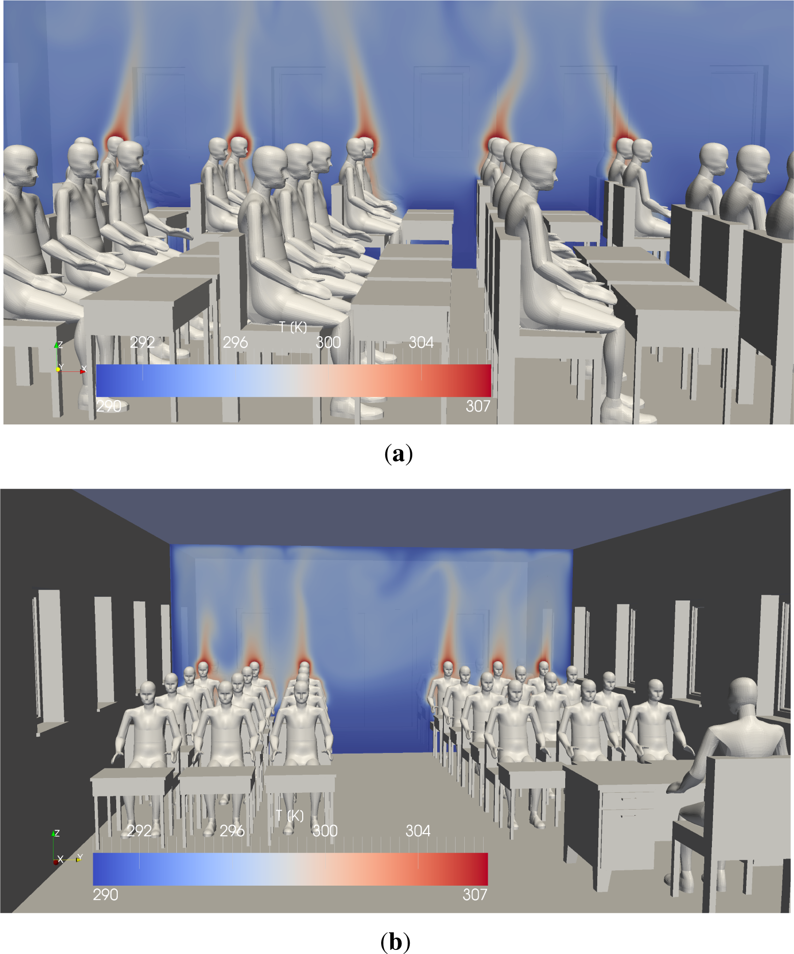
Figure 14 shows an overview of the classroom and two characteristic temperature slices through the domain, while Figure 15 shows two details from different viewing angles. The rising heat plumes over the heads of the students can be observed exceptionally well. Furthermore, it can be seen that the different plumes of the students interact with each other and have quite a significant influence on each other. The thermal plume over the teacher, however, is nearly not affected by such interactions.

Figure 16 shows cut-lines over every student, starting immediately above the head and going 1 m straight up into the air. The plot does not currently display which line belongs to which student in order to keep it readable and to avoid overloading it with textual information. The most important information that can be gathered from this plot is the fact that the classroom scenario has highly complex 3D flow properties. Thirty centimeters above the head of a student, temperature differences in the order of 8 °C could be observed. It should be mentioned at this place that in order to visualize the temperature values displayed in Figure 16, the data were extracted at a higher level in the data structure in order to cope with the large amount of data available at the deepest level. However, this procedure automatically introduces an averaging process due to the nature of the data structure itself, and thus, local fluctuations are smoothed in the process for the scope of visualization, which does not affect the overall solution.

Furthermore, asymmetries can be clearly seen in Figure 15b. While the student sitting in the middle between two colleagues is much better ‘isolated’, the student sitting next to the corridor is exposed to cooler air on the isle side.

As shown in the paper of Urlaub et al. [46], the indoor climate can have a significant impact on the occupants’ working performance, as well as their health. As the simulations indicate, the usage of one global indoor temperature might be very inaccurate in order to assess the possible human performance effects in a classroom.

Further possible assessments regarding indoor thermal comfort can be made by evaluating the local mean votes (LMV), as described by van Treeck et al. [47]. The LMVs can be generated for different body sectors of different students at different locations in the classroom. Hence, efficient hybrid ventilation scenarios, specifically designed to account for a complete classroom, could be devised in order to counteract negative impacts from a pure natural airflow in the room. Furthermore, additional transport equations could be coupled to the thermal simulations, enabling the monitoring of CO₂ concentrations or ‘air age’ in buildings of this type.

Hence, a broad variety of different evaluation routines or post-processing tools could be used, building on the generated results from different high-performance simulation runs.

6. Conclusions

This paper presented a data structure capable of running efficiently on modern supercomputers, such as SuperMUC in Germany or Shaheen in the Kingdom of Saudi Arabia, and which is able to compute complex indoor airflow scenarios. The mathematical formulations based on the Navier–Stokes equations for the simulation of indoor airflows were introduced, and the basic ideas of the data structure, as well as the solving mechanisms were sketched. Scaling plots showed the efficient usage of the introduced strategies on SuperMUC and Shaheen. Furthermore, validation examples and complex indoor airflow scenarios were presented in order to highlight the possibilities that the code currently provides.

Moreover, it is planned to enhance the existing code structure with further features, such as turbulence modeling and immersed boundary methods for a more accurate geometric description. The porting of parts of the code to hardware accelerators could also enhance the performance greatly and enable a more efficient execution on supercomputers drawing most of their computing resources from accelerator hardware, such as graphic cards or the Intel Xeon Phi architecture. Larger examples can be targeted or an increase in resolution of the already available ones could be performed using the same amount of time.