Two-Dimensional Anomalous Solute Transport in a Two-Zone Fractal Porous Medium

Abstract

This study addresses a two-dimensional anomalous solute transport process within a two-zone fractal porous medium. A mathematical formulation is developed to characterise transport phenomena in a non-homogeneous porous domain. The medium consists of two interacting regions: one containing mobile fluid and the other containing immobile fluid, between which mass transfer occurs. In the mobile-fluid region, solute transport is governed by the convection–diffusion equation. In contrast, the immobile-fluid region is described using a first-order kinetic model. The problem of solute injection through a designated boundary point is formulated and numerically implemented. The effects of anomalous transport behaviour on solute migration and filtration characteristics are examined. The study further evaluates the pressure field, filtration velocity distribution, and solute concentration in both zones.

1. Introduction

In recent decades, fractional differential equations have emerged as powerful tools for modelling complex processes across many scientific and engineering disciplines. Their growing application is largely due to their flexibility and ability to represent nonlinear behaviour, time-dependent parameter variations, and memory effects features that are often inadequately described by classical differential equations. Porous media are frequently conceptualised as systems composed of two interacting regions: one containing mobile fluid and the other containing immobile fluid [1]. It is commonly assumed that diffusive mass exchange between these regions is proportional to the concentration difference between them. Sorption in both regions is considered instantaneous, and adsorption is represented using a linear isotherm. The corresponding analytical formulation captures the tailing behaviour observed in breakthrough curves for flows through unsaturated aggregated sorbing media and explains the frequently reported early solute breakthrough. The problem of anomalous filtration and solute transport in a dual-zone porous medium with a strip source was formulated and numerically investigated in [2]. In that study, anomalous convective diffusive transport was assumed in one region, while purely diffusive transport occurred in the other. A filtration model treating the porous structure as a fractal body was introduced in [3]. The medium geometry was described through gaps between contacting rough and wavy surfaces, consisting of pore spaces and contact zones. Approaches for determining fractal dimensions related to tortuosity and porosity were developed, and relationships linking leakage characteristics and fractal dimension with tortuosity and porosity of a compacted medium were established.

Fractal-based porous media models constructed using fractional-dimension sets were presented in [4], including examples involving geomaterials. Scaling relationships governing porosity, permeability, and pore and grain size distributions were derived. The influence of external factors, such as pressure, on the properties of fractal porous structures was also examined. A numerical technique for solving the two-dimensional subdiffusion equation with a Caputo fractional derivative was proposed in [5]. By assuming symmetry in both the solution domain and boundary conditions, the two-dimensional problem was reduced to a one-dimensional form. The method extends the fractional Crank–Nicolson approach through discretisation of an equivalent integro-differential formulation. In ref. [6], a hybrid computational scheme combining a weighted finite difference method with a fifth-order Hermite collocation technique was introduced. This approach was applied to a time-variable fractional advection–dispersion model, employing Hermite splines for spatial discretization and weighted finite differences in time. The study in [7] assumed that convective–dispersive transport occurs exclusively in the mobile-fluid region, while solute exchange between mobile and immobile zones follows first-order kinetics. The solid matrix was divided into two types of adsorption sites corresponding to mobile and immobile liquid regions, both assumed to be in instantaneous equilibrium. Adsorption was modelled using a linear isotherm, and first-order degradation was considered in both liquid and solid phases. Distinct degradation coefficients were introduced for mobile and immobile regions and their associated adsorbed phases to preserve generality.

The application of fractional differential equations to describe anomalous solute transport in two-zone porous media containing macro- and micropores was discussed in [8,9]. That work included numerical simulations and analysis of how the fractal structure of the medium affects transport behaviour. Multi-term time-fractional diffusion equations were numerically solved in a bounded domain in [10], where solute concentration distributions were determined. The influence of both spatial and temporal fractional orders representing fractal characteristics of the medium on transport dynamics was examined, including cases involving multiple time-derivative terms. Anomalous solute transport in a cylindrical two-zone fractal porous medium was analysed in [11], demonstrating how fractal geometry modifies transport characteristics through advanced mathematical modelling. In ref. [12], anomalous transport in a two-dimensional fractal porous medium was studied with dispersion coefficients and filtration velocity varying in both space and time. Transport anomalies were incorporated via fractional spatial derivatives in the diffusion terms, linking anomalous behaviour to the medium’s fractal structure. Two-dimensional anomalous filtration and transport problems were numerically investigated in [13], where the porous medium was assumed to exhibit fractal properties. A fractional-order piezo conductivity equation derived from anomalous Darcy’s law, combined with porosity, density, and continuity relations, was formulated. An analytical solution for one-dimensional solute transport in an idealised homogeneous medium was obtained in [14]. However, realistic transport processes often depend on spatial variability, requiring the consideration of position-dependent dispersion and velocity. Certain one-dimensional inhomogeneous cases were solved in [15], while more complex and two-dimensional configurations necessitated numerical approaches [16,17]. An explicit finite-difference solution for a one-dimensional advection–dispersion equation with variable coefficients was developed, and later extended, to two-dimensional semi-infinite domains [18,19].

A two-dimensional transport model for a semi-infinite inhomogeneous porous medium was formulated in [20]. The formation was assumed to initially contain solute, with contamination introduced from a pulsed point source varying in space and time. The dispersion coefficient was modelled as proportional to both a spatial function and seepage velocity, with the latter expressed as a power of the spatial variable. Exponentially decaying and sinusoidal velocity profiles were examined. The effects of retardation, spatial variability, and temporal dependence on solute concentration were analysed. By introducing transformed independent variables, the governing equation was reduced to constant coefficients and solved using Laplace transforms. Parameter influences were illustrated graphically.

In the present study, anomalous solute transport in a heterogeneous two-zone porous medium is investigated. Mass exchange occurs between the mobile and immobile regions. The immobile-fluid zone is described by a kinetic equation incorporating anomalous effects, while the mobile-fluid region is governed by a convection–diffusion equation that accounts for anomalous diffusion behaviour. A two-dimensional semi-infinite domain is considered, and the transport problem is solved numerically. The effects of anomalous diffusion and interzonal mass-transfer kinetics on overall transport characteristics are evaluated. Here, anomalous transport refers to deviations from classical diffusion and convection laws, necessitating fractional or non-classical formulations to adequately describe filtration and solute migration processes.

2. Problem Statement and the Method of Solution

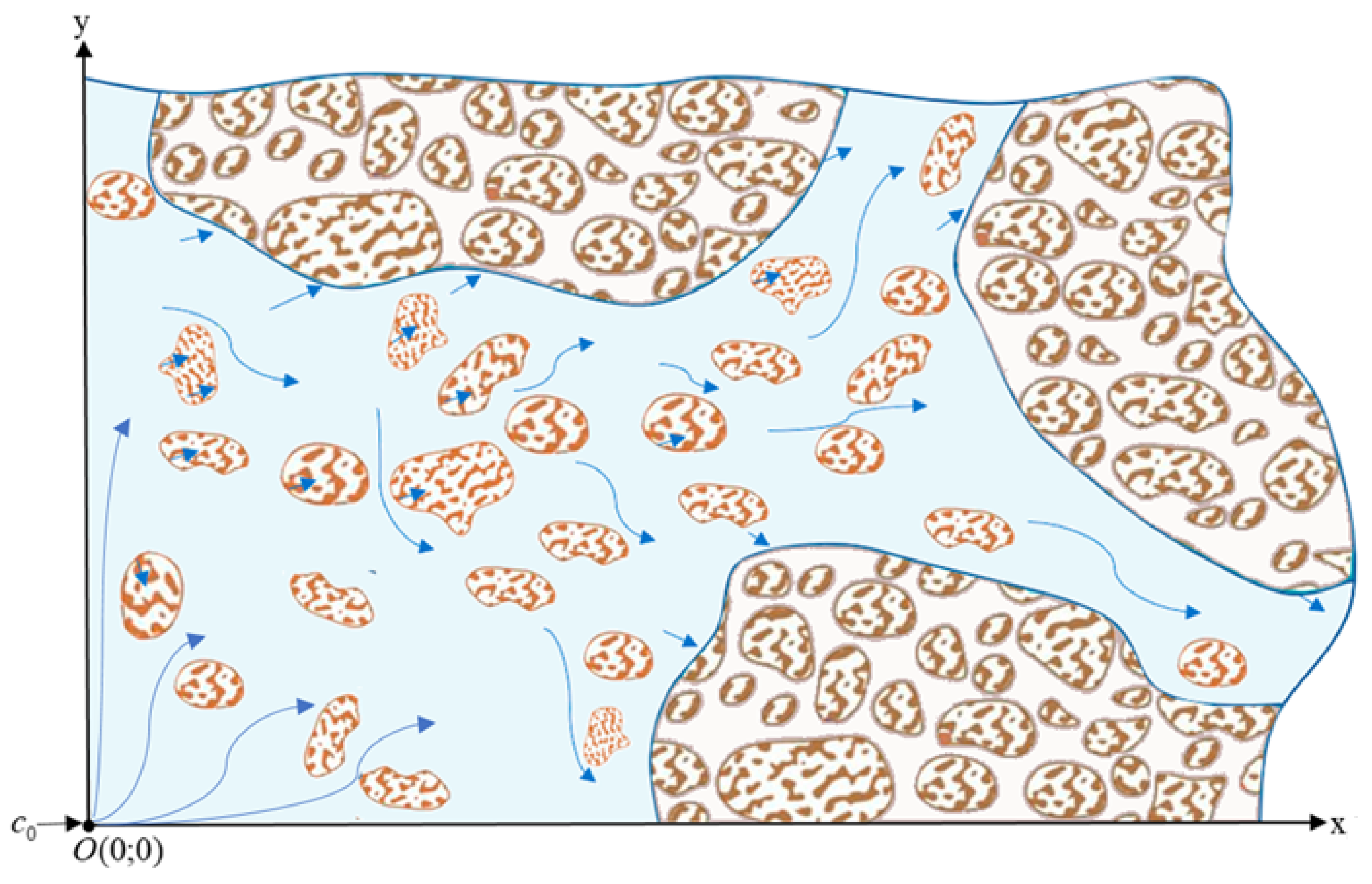
The considered porous medium comprises two interacting regions: a mobile-fluid zone and an immobile-fluid zone. Fluid flow occurs in the mobile region, while in the immobile region the fluid is at rest; however, molecular diffusion between the zones is allowed. The analysis is carried out in a rectangular semi-infinite domain (Figure 1). Initially, the domain is assumed to be completely saturated with clean fluid, free of solute. In this case, the equilibrium equation is written in the two-dimensional form [1,21,22,23] as

$${\mathrm{\theta }}_m{\displaystyle \frac{\mathsf{\partial }{c}_m}{\mathsf{\partial }t}}+\mathrm{\gamma }{\mathrm{\theta }}_{im}{\displaystyle \frac{{\mathsf{\partial }}^{\mathrm{\alpha }}{c}_{im}}{\mathsf{\partial }{t}^{\mathrm{\alpha }}}}={\mathrm{\theta }}_m\left(D_{mx}{\displaystyle \frac{{\mathsf{\partial }}^{\mathrm{\beta }}{c}_m}{\mathsf{\partial }{x}^{\mathrm{\beta }}}}+D_{my}{\displaystyle \frac{{\mathsf{\partial }}^{\mathrm{\beta }}{c}_m}{\mathsf{\partial }{y}^{\mathrm{\beta }}}}\right)-v_{mx}{\mathrm{\theta }}_m{\displaystyle \frac{\mathsf{\partial }{c}_m}{\mathsf{\partial }x}}-v_{my}{\mathrm{\theta }}_m{\displaystyle \frac{\mathsf{\partial }{c}_m}{\mathsf{\partial }y}}$$

(1)

where ${\mathrm{\theta }}_m,{\mathrm{\theta }}_{im}$ are porosity, $c_m,c_{im}$ are volumetric concentrations of the substance, $D_{mx},D_{my}$ are the coefficients of hydrodynamic dispersion in the moving zone, $v_{mx},v_{my}$ are the average velocities, the index $m$ corresponds to the mobile zone, and the index $im$ corresponds to the immobile zone.

The presence of a stagnant (immobile) zone is considered based on the kinetic equation

$$\mathrm{\gamma }{\mathrm{\theta }}_{im}{\displaystyle \frac{{\mathsf{\partial }}^{\mathrm{\alpha }}{c}_{im}}{\mathsf{\partial }{t}^{\mathrm{\alpha }}}}=\mathrm{\omega }\left(c_m-c_{im}\right)$$

(2)

where $\mathrm{\gamma }$ is the mass transfer coefficient, $\left[\mathrm{\gamma }\right]=T^{\mathrm{\alpha }-1},$$\left[\mathrm{\omega }\right]=T^{-1}.$

The orders of fractional derivatives $\mathrm{\alpha }$ and $\mathrm{\beta }$ are taken in the following range: $0<\mathrm{\alpha }\le 1,$ $1<\mathrm{\beta }\le 2.$

Here, the initial and boundary conditions are considered as follows:

$$c_m(0,x,y)=0,$$

(3)

$$c_{im}(0,x,y)=0.$$

(4)

$$c_m(t,0,0)=c_0,c_0=const$$

(5)

$${\displaystyle \frac{\mathsf{\partial }{c}_m(t,\infty ,y)}{\mathsf{\partial }x}}=0,$$

(6)

$${\displaystyle \frac{\mathsf{\partial }{c}_m(t,0,y)}{\mathsf{\partial }x}}=0,y>0,$$

(7)

$${\displaystyle \frac{\mathsf{\partial }{c}_m(t,x,0)}{\mathsf{\partial }y}}=0,$$

(8)

$${\displaystyle \frac{\mathsf{\partial }{c}_m(t,x,\infty )}{\mathsf{\partial }y}}=0.$$

(9)

The pressure and filtration velocity fields are obtained by applying an anomalous filtration equation developed from anomalous Darcy’s law.

$${\displaystyle \frac{\mathsf{\partial }p}{\mathsf{\partial }t}}={\mathrm{\chi }}_x{\displaystyle \frac{{\mathsf{\partial }}^{1+{\mathrm{\delta }}_1}p}{\mathsf{\partial }{x}^{1+{\mathrm{\delta }}_1}}}+{\mathrm{\chi }}_y{\displaystyle \frac{{\mathsf{\partial }}^{1+{\mathrm{\delta }}_2}p}{\mathsf{\partial }{y}^{1+{\mathrm{\delta }}_2}}},{\mathrm{\chi }}_x={\displaystyle \frac{k_x}{\mathrm{\mu }{\mathrm{\beta }}^{\ast }}},{\mathrm{\chi }}_y={\displaystyle \frac{k_y}{\mathrm{\mu }{\mathrm{\beta }}^{\ast }}}$$

(10)

where ${\mathrm{\chi }}_x$, ${\mathrm{\chi }}_y$ are piezo conductivity coefficients in the $x$ and $y$ directions respectively; ${\mathrm{\beta }}^{\ast }$ is the coefficient of elastic capacity of the medium; and ${\mathrm{\delta }}_1,$${\mathrm{\delta }}_2$ are the orders of the derivative.

Equation (1) is derived from Darcy’s anomalous laws

$$v_{mx}=-{\displaystyle \frac{k_x}{\mathrm{\mu }}}{\displaystyle \frac{{\mathsf{\partial }}^{{\mathrm{\delta }}_1}p}{\mathsf{\partial }{x}^{{\mathrm{\delta }}_1}}},$$

(11)

$$v_{my}=-{\displaystyle \frac{k_y}{\mathrm{\mu }}}{\displaystyle \frac{{\mathsf{\partial }}^{{\mathrm{\delta }}_2}p}{\mathsf{\partial }{y}^{{\mathrm{\delta }}_2}}},$$

(12)

Here, $k_x,$ $k_y$ are the permeability coefficients in the $x$ and $y$ directions respectively.

In (10), (11): $0\le {\mathrm{\delta }}_1,$ ${\mathrm{\delta }}_2\le 1.$

For Equation (10), the following initial and boundary conditions are fixed as [13]:

$$p(0,x,y)=0,$$

(13)

$$p(t,0,0)=p_0=const,$$

(14)

$${\displaystyle \frac{{\mathsf{\partial }}^{{\mathrm{\delta }}_1}p(t,0,y)}{\mathsf{\partial }{x}^{{\mathrm{\delta }}_1}}}=0,y>0,$$

(15)

$${\displaystyle \frac{{\mathsf{\partial }}^{{\mathrm{\delta }}_1}p(t,\infty ,y)}{\mathsf{\partial }{x}^{{\mathrm{\delta }}_1}}}=0,(orp(t,\infty ,y)=0),$$

(16)

$${\displaystyle \frac{{\mathsf{\partial }}^{{\mathrm{\delta }}_2}p(t,x,0)}{\mathsf{\partial }{y}^{{\mathrm{\delta }}_2}}}=0,x>0,{\displaystyle \frac{{\mathsf{\partial }}^{{\mathrm{\delta }}_2}p(t,x,\infty )}{\mathsf{\partial }{y}^{{\mathrm{\delta }}_2}}}=0(orp(t,x,\infty )=0),x>0.$$

(17)

We have adopted a numerical method to solve Equations (1)–(17) and applied the finite difference method [24] to analyse the study.

In the domain $\mathrm{\Omega }=\left\{0\le x\le \infty ,0\le y\le \infty ,0\le t\le t_{\max }\right\}$, we introduce a uniform grid ${\mathrm{\omega }}_{h_1{h}_2\mathrm{\tau }}=\left\{\left(t_k,x_i,y_j\right),x_i=i{h}_1,y_j=j{h}_2,t_k=k\mathrm{\tau },\mathrm{\tau }=t_{\max }/K,i=0,1,2\dots ,j=0,1,2\dots ,k=\overline{0,K}\right\}$, where $h_1$ is the grid step in the direction $x$, $h_2$ is the grid step in the direction $y$, $\mathrm{\tau }$ is the grid step by time $t$, $t_{\max }$ is the maximum time during which the process is studied, $K$ is the number of grid intervals by $t$.

Instead of the functions $c(t,x,y)$, $v(t,x,y)$, and $p(t,x,y)$, we consider the grid functions $v_{ij}^k$, $p_{ij}^k$, and $c_{ij}^k$ at the nodes $(t_k,x_i,y_j)$.

On the grid ${\mathrm{\omega }}_{h_1{h}_2\mathrm{\tau }}$, we approximate Equations (1) and (2) as follows:

$$\begin{array}{l}{\displaystyle \frac{{\mathrm{\theta }}_m\left({(c_m)}_{i,j}^{k+1}-{(c_m)}_{i,j}^k\right)}{\mathrm{\tau }}}\\ +{\displaystyle \frac{{\mathrm{\theta }}_{im}\mathrm{\gamma }}{\Gamma (2-\mathrm{\alpha }){\mathrm{\tau }}^{\mathrm{\alpha }}}}\left[{\displaystyle \sum _{l=0}^{k-1}\left({(c_{im})}_{i,j}^{l+1}-{(c_{im})}_{i,j}^l\right)·\left({\left(k-l+1\right)}^{1-\mathrm{\alpha }}-{\left(k-l\right)}^{1-\mathrm{\alpha }}\right)+\left({(c_{im})}_{i,j}^{k+1}-{(c_{im})}_{i,j}^k\right)}\right]=\\ ={\displaystyle \frac{{\mathrm{\theta }}_m{D}_{mx}}{\mathrm{\Gamma }\left(3-\mathrm{\beta }\right)h_1^{\mathrm{\beta }}}}{\displaystyle \sum _{l=0}^{i-1}\left({\left(c_m\right)}_{i-(l-1),j}^k-2{\left(c_m\right)}_{i-l,j}^k+{\left(c_m\right)}_{i-\left(l+1\right),j}^k\right)}\left({\left(l+1\right)}^{2-\mathrm{\beta }}-l^{2-\mathrm{\beta }}\right)\\ +{\displaystyle \frac{{\mathrm{\theta }}_m{D}_{my}}{\mathrm{\Gamma }\left(3-\mathrm{\beta }\right)h_2^{\mathrm{\beta }}}}{\displaystyle \sum _{l=0}^{j-1}\left({\left(c_m\right)}_{i,j-(l-1)}^k-2{\left(c_m\right)}_{i,j-l}^k+{\left(c_m\right)}_{i,j-\left(l+1\right)}^k\right)}\left({\left(l+1\right)}^{2-\mathrm{\beta }}-l^{2-\mathrm{\beta }}\right)\\ -v_{mx}{\mathrm{\theta }}_m{\displaystyle \frac{{\left(c_m\right)}_{i,j}^k-{\left(c_m\right)}_{i-1,j}^k}{h_1}}-v_{my}{\mathrm{\theta }}_m{\displaystyle \frac{{\left(c_m\right)}_{i,j}^k-{\left(c_m\right)}_{i,j-1}^k}{h_2}},\end{array}$$

(18)

$$\begin{array}{l}{(c_m)}_{ij}^{k+1}={\displaystyle \frac{\mathrm{\tau }{D}_{mx}}{\mathrm{\Gamma }\left(3-\mathrm{\beta }\right)h_1^{\mathrm{\beta }}}}{\displaystyle \sum _{l=0}^{i-1}\left({\left(c_m\right)}_{i-(l-1),j}^k-2{\left(c_m\right)}_{i-l,j}^k+{\left(c_m\right)}_{i-\left(l+1\right),j}^k\right)}\left({\left(l+1\right)}^{2-\mathrm{\beta }}-l^{2-\mathrm{\beta }}\right)\\ +{\displaystyle \frac{\mathrm{\tau }{D}_{my}}{\mathrm{\Gamma }\left(3-\mathrm{\beta }\right)h_2^{\mathrm{\beta }}}}{\displaystyle \sum _{l=0}^{j-1}\left({\left(c_m\right)}_{i,j-(l-1)}^k-2{\left(c_m\right)}_{i,j-l}^k+{\left(c_m\right)}_{i,j-\left(l+1\right)}^k\right)}\left({\left(l+1\right)}^{2-\mathrm{\beta }}-l^{2-\mathrm{\beta }}\right)\\ -{\displaystyle \frac{\mathrm{\tau }{v}_{mx}\left({\left(c_m\right)}_{i,j}^k-{\left(c_m\right)}_{i-1,j}^k\right)}{h_1}}-{\displaystyle \frac{\mathrm{\tau }{v}_{my}\left({\left(c_m\right)}_{i,j}^k-{\left(c_m\right)}_{i,j-1}^k\right)}{h_2}}+{(c_m)}_{ij}^k\\ -{\displaystyle \frac{\mathrm{\tau }{\mathrm{\theta }}_{im}\mathrm{\gamma }}{{\mathrm{\theta }}_m\Gamma (2-\mathrm{\alpha }){\mathrm{\tau }}^{\mathrm{\alpha }}}}\left[{\displaystyle \sum _{l=0}^{k-1}\left({(c_{im})}_{i,j}^{l+1}-{(c_{im})}_{i,j}^l\right)·\left({\left(k-l+1\right)}^{1-\mathrm{\alpha }}-{\left(k-l\right)}^{1-\mathrm{\alpha }}\right)+\left({(c_{im})}_{i,j}^{k+1}-{(c_{im})}_{i,j}^k\right)}\right].\end{array}$$

(19)

$$\begin{array}{l}\mathrm{\gamma }{\mathrm{\theta }}_{im}{\displaystyle \frac{{\mathrm{\tau }}^{1-\mathrm{\alpha }}}{\Gamma (2-\mathrm{\alpha })}}\left[{\displaystyle \sum _{l=0}^{k-1}\frac{{(c_{im})}_{i,j}^{l+1}-{(c_{im})}_{i,j}^l}{\mathrm{\tau }}·\left({\left(k-l+1\right)}^{1-\mathrm{\alpha }}-{\left(k-l\right)}^{1-\mathrm{\alpha }}\right)+\frac{{(c_{im})}_{i,j}^{k+1}-{(c_{im})}_{i,j}^k}{\mathrm{\tau }}}\right]=\\ =\mathrm{\omega }\left({\left(c_m\right)}_{i,j}^k-{\left(c_{im}\right)}_{i,j}^k\right),\end{array}$$

(20)

$$\begin{array}{l}{(c_{im})}_{i,j}^{k+1}={\displaystyle \frac{\Gamma (2-\mathrm{\alpha }){\mathrm{\tau }}^{\mathrm{\alpha }}\mathrm{\omega }}{{\mathrm{\theta }}_{im}\mathrm{\gamma }}}·\left({\left(c_m\right)}_{i,j}^k-{\left(c_{im}\right)}_{i,j}^k\right)\\ -{\displaystyle \sum _{l=0}^{k-1}\left({(c_{im})}_{i,j}^{l+1}-{(c_{im})}_{i,j}^l\right)·\left({\left(k-l+1\right)}^{1-\mathrm{\alpha }}-{\left(k-l\right)}^{1-\mathrm{\alpha }}\right)}+{(c_{im})}_{i,j}^k.\end{array}$$

(21)

Equation (10) is approximated as

$$\begin{array}{l}{\displaystyle \frac{p_{ij}^{k+1}-p_{ij}^k}{\mathrm{\tau }}}={\displaystyle \frac{{\mathrm{\chi }}_x}{\mathrm{\Gamma }\left(3-{\mathrm{\delta }}_1\right)h_1^{{\mathrm{\delta }}_1}}}{\displaystyle \sum _{l=0}^{i-1}\left(p_{i-(l-1),j}^k-2p_{i-l,j}^k+p_{i-\left(l+1\right),j}^k\right)}\left({\left(l+1\right)}^{2-{\mathrm{\delta }}_1}-l^{2-{\mathrm{\delta }}_1}\right)\\ +{\displaystyle \frac{{\mathrm{\chi }}_y}{\mathrm{\Gamma }\left(3-{\mathrm{\delta }}_2\right)h_2^{{\mathrm{\delta }}_2}}}{\displaystyle \sum _{l=0}^{j-1}\left(p_{i,j-(l-1)}^k-2p_{i,j-l}^k+p_{i,j-\left(l+1\right)}^k\right)}\left({\left(l+1\right)}^{2-{\mathrm{\delta }}_2}-l^{2-{\mathrm{\delta }}_2}\right),\end{array}$$

(22)

$$\begin{array}{l}{p}_{i,j}^{k+1}={\displaystyle \frac{\mathrm{\tau }·{\mathrm{\chi }}_x}{\mathrm{\Gamma }\left(3-{\mathrm{\delta }}_1\right)h_1^{{\mathrm{\delta }}_1}}}{\displaystyle \sum _{l=0}^{i-1}\left(p_{i-(l-1),j}^k-2p_{i-l,j}^k+p_{i-\left(l+1\right),j}^k\right)}\left({\left(l+1\right)}^{2-{\mathrm{\delta }}_1}-l^{2-{\mathrm{\delta }}_1}\right)\\ +{\displaystyle \frac{\mathrm{\tau }·{\mathrm{\chi }}_y}{\mathrm{\Gamma }\left(3-{\mathrm{\delta }}_2\right)h_2^{{\mathrm{\delta }}_2}}}{\displaystyle \sum _{l=0}^{j-1}\left(p_{i,j-(l-1)}^k-2p_{i,j-l}^k+p_{i,j-\left(l+1\right)}^k\right)}\left({\left(l+1\right)}^{2-{\mathrm{\delta }}_2}-l^{2-{\mathrm{\delta }}_2}\right)+p_{i,j}^k.\end{array}$$

(23)

The components of the filtration velocity are approximated as follows Equations (11) and (12):

$${\left(v_{mx}\right)}_{ij}^{k+1}=-{\displaystyle \frac{k_x}{\mathrm{\mu }}}{\displaystyle \frac{p_{i+1j}^{k+1}-{\mathrm{\delta }}_1{p}_{i,j}^{k+1}}{\Gamma (2-{\mathrm{\delta }}_1)h_1^{{\mathrm{\delta }}_1}}},$$

(24)

$${\left(v_{my}\right)}_{ij}^k=-{\displaystyle \frac{k_y}{\mathrm{\mu }}}{\displaystyle \frac{p_{ij+1}^k-{\mathrm{\delta }}_2{p}_{i,j}^k}{\Gamma (2-{\mathrm{\delta }}_2)h_2^{{\mathrm{\delta }}_2}}}.$$

(25)

The initial conditions, as described in Equations (3) and (4), are approximated as follows:

$${\left(c_m\right)}_{i,j}^k=0,$$

(26)

$${\left(c_{im}\right)}_{i,j}^k=0.$$

(27)

The boundary conditions, specifically Equations (5) and (9), are approximated as follows:

$${\left(c_m\right)}_{i,j}^k=c_0,$$

(28)

$${\displaystyle \frac{{\left(c_m\right)}_{i,j}^k-{\left(c_m\right)}_{i-1,j}^k}{h_1}}=0,$$

(29)

$${\displaystyle \frac{{\left(c_m\right)}_{i+1,j}^k-{\left(c_m\right)}_{i,j}^k}{h_1}}=0,$$

(30)

$${\displaystyle \frac{{\left(c_m\right)}_{i,j+1}^k-{\left(c_m\right)}_{i,j}^k}{h_2}}=0,$$

(31)

$${\displaystyle \frac{{\left(c_m\right)}_{i,j-1}^k-{\left(c_m\right)}_{i,j}^k}{h_2}}=0,$$

(32)

Approximations of Equations (13)–(17) have the form

$$p_{i,j}^k=0,$$

(33)

$$p_{i,j}^k=p_0,$$

(34)

$${\displaystyle \frac{p_{i+1,j}^k-{\mathrm{\delta }}_1{p}_{i,j}^k}{\mathrm{\Gamma }\left(2-{\mathrm{\delta }}_1\right)h_1^{{\mathrm{\delta }}_1}}}=0,$$

(35)

$${\displaystyle \frac{p_{i,j}^k-{\mathrm{\delta }}_1{p}_{i-1,j}^k}{\mathrm{\Gamma }\left(2-{\mathrm{\delta }}_1\right)h_1^{{\mathrm{\delta }}_1}}}=0,(\mathrm{or}{p}_{i,j}^k=0),$$

(36)

$${\displaystyle \frac{p_{i,j+1}^k-{\mathrm{\delta }}_2{p}_{i,j}^k}{\mathrm{\Gamma }\left(2-{\mathrm{\delta }}_2\right)h_2^{{\mathrm{\delta }}_2}}}=0,x>0,$$

(37)

$${\displaystyle \frac{p_{i,j}^k-{\mathrm{\delta }}_2{p}_{i,j-1}^k}{\mathrm{\Gamma }\left(2-{\mathrm{\delta }}_2\right)h_2^{{\mathrm{\delta }}_2}}}=0,(\mathrm{or}{p}_{i,j}^k=0),x>0.$$

(38)

3. Results and Discussion

To obtain numerical results, the following initial values of parameters are used: $c_0=0.01$, $D_{mx}=4\times {10}^{-5}$, $D_{my}=5\times {10}^{-5}$, ${\mathrm{\theta }}_m=0.4$, ${\mathrm{\theta }}_{im}=0.1$, $\mathrm{\omega }={10}^{-7}$$T^{-1}$, $\mathrm{\gamma }=0.6$$T^{\mathrm{\alpha }-1}$, $p_0={10}^{5}Pa$, $k_x={10}^{-13}$${\mathrm{m}}^{{\mathrm{\delta }}_1}$, $k_y=2\times {10}^{-13}$${\mathrm{m}}^{{\mathrm{\delta }}_2},$$\mu =5\times {10}^{-3}$$Pa·s,$${\beta }^{\ast }=3\times {10}^{-8}$$P{a}^{-1}$.

The convergence results are studied for the number of intervals along the x axis (I) and number of intervals along the y axis (J). The results are computed for I, J = 10, 20, and 30 by fixing the values $\mathrm{\beta }=2$, ${\mathrm{\delta }}_1=1$, ${\mathrm{\delta }}_2=1,$$t=2400$ s The results of the 25th grid point for I, J = 10, 20, and 30 are 0.0021, 0.0020656731, and 0.0020656721 respectively. The percentile changes in the values for I, J = 20 and 30 are 0.01%. So, it is fixed as I = J = 30 for the analysis of the problem for all results.

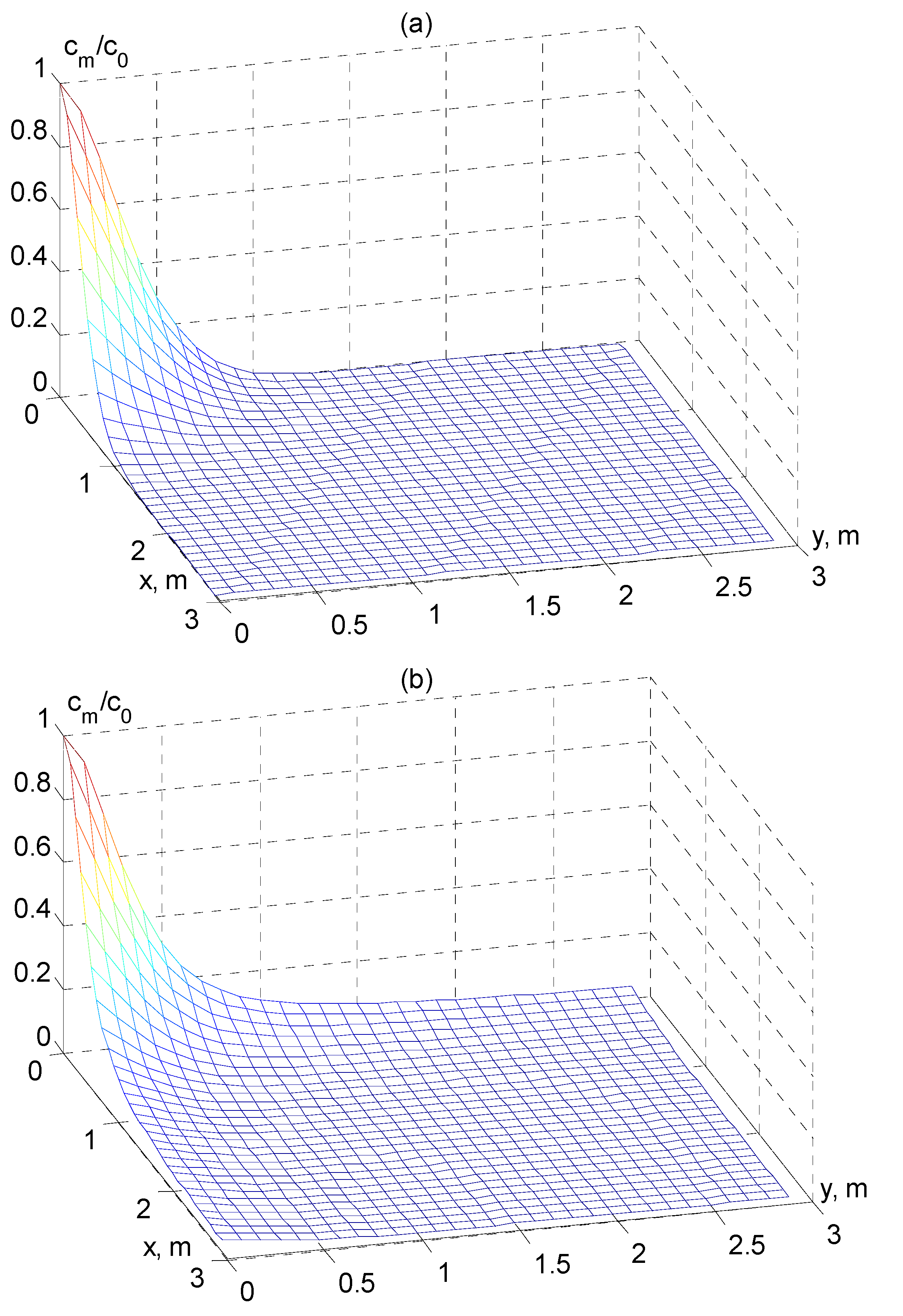
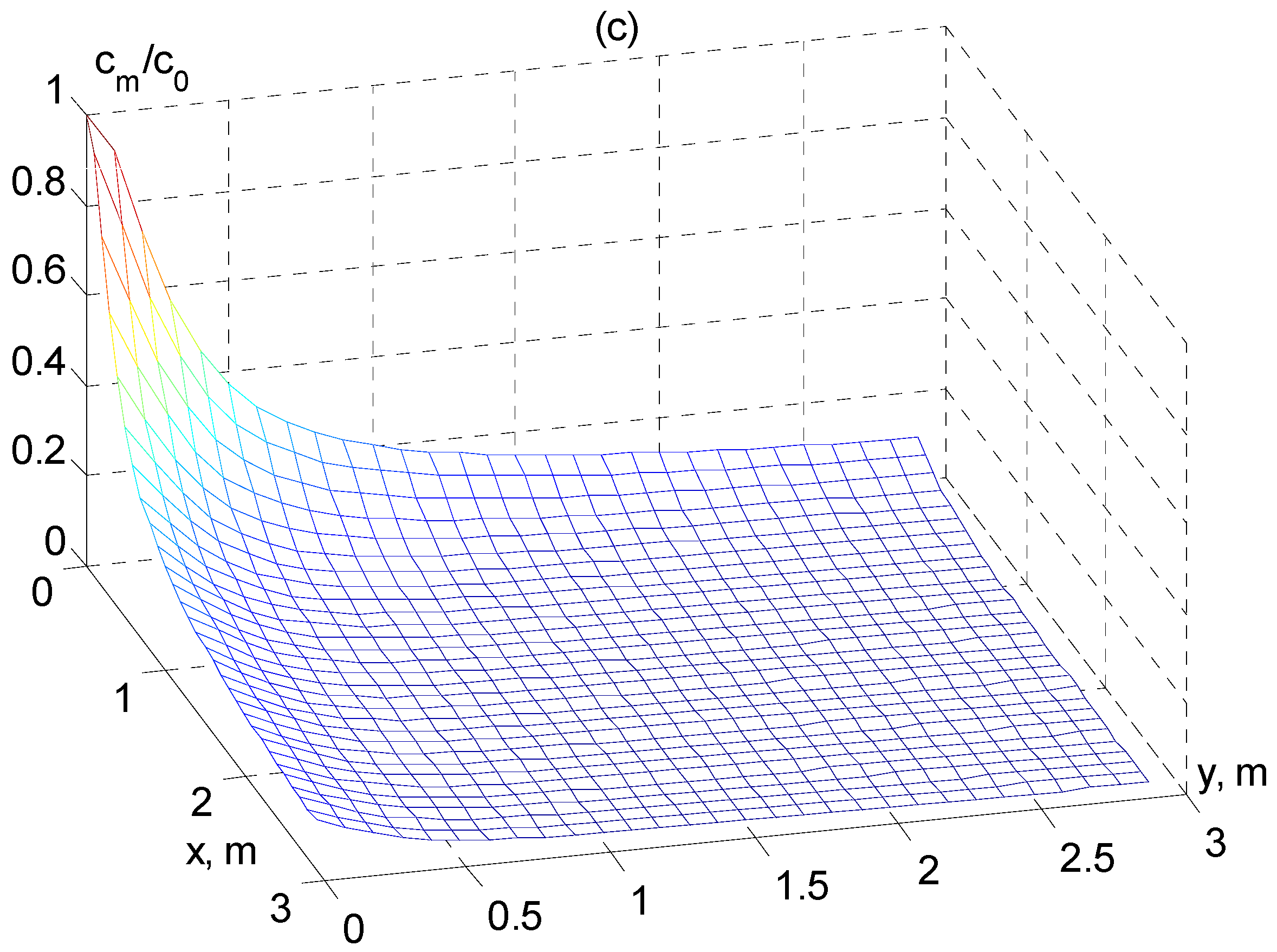
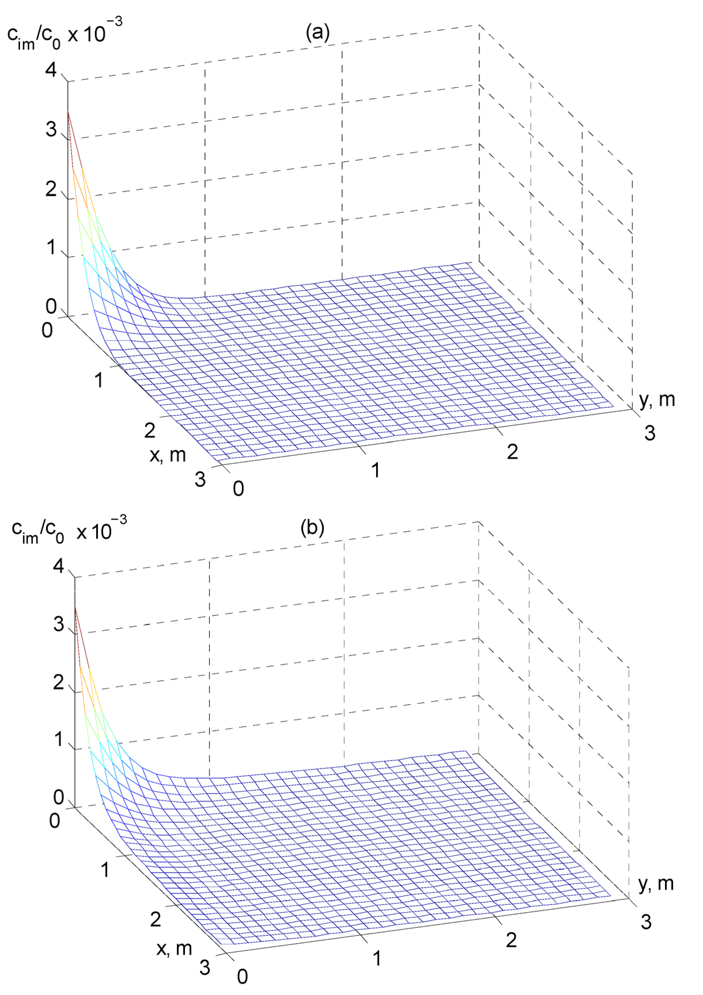
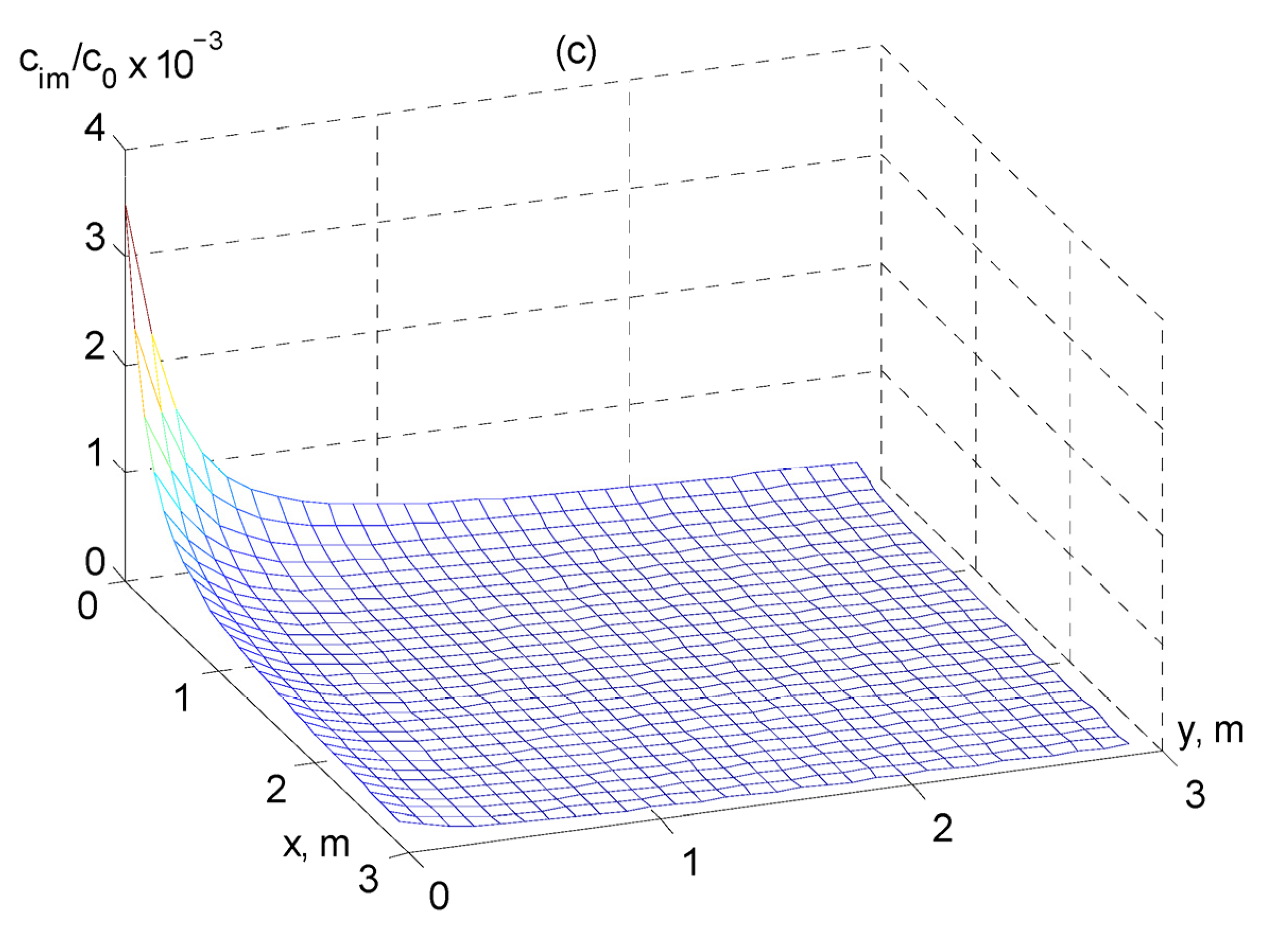
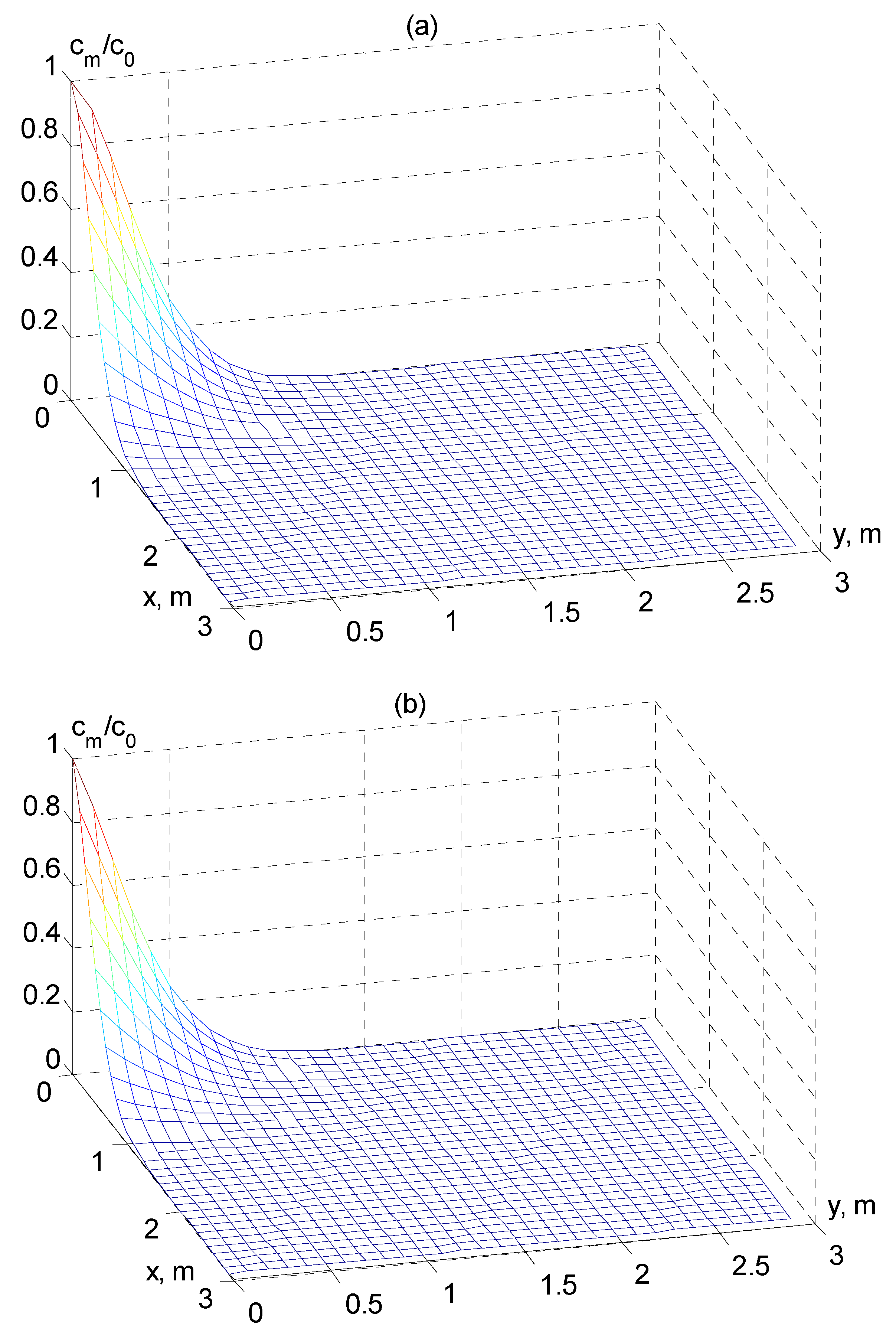
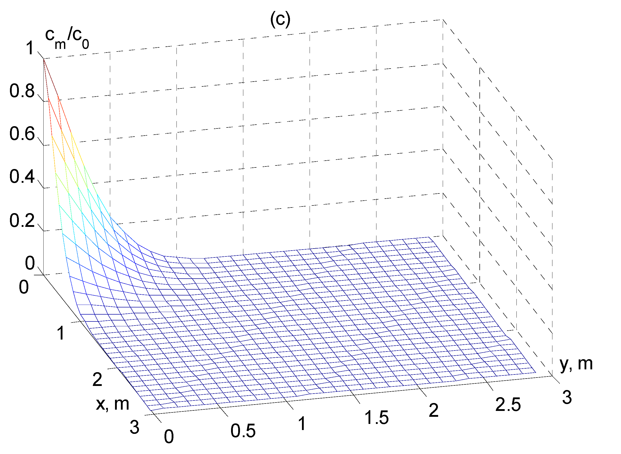
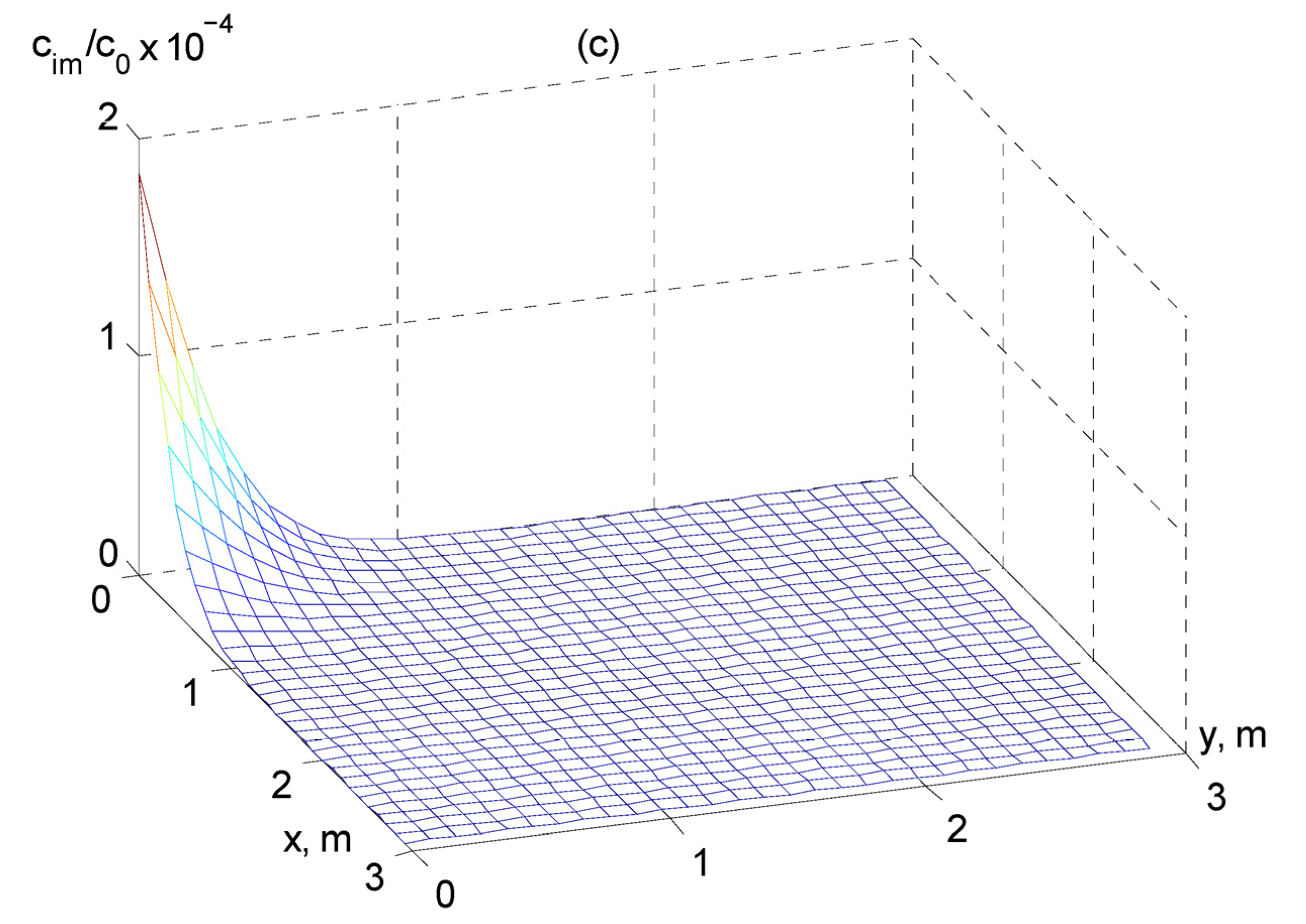
Figure 2 and Figure 3 show the variation in the concentration surfaces $c_m$ and $c_{im}$, respectively, for fixed values of $\mathrm{\alpha }=1$, ${\mathrm{\delta }}_1=1$, ${\mathrm{\delta }}_2=1,$$t=2400$ s with different values of $\mathrm{\beta }=2$ (Figure 2a), $\mathrm{\beta }=1.8$ (Figure 2b), and $\mathrm{\beta }=1.6$ (Figure 2c). In these figures, the results show that with the decrease in the derivatives order $\beta$ from 2, the fast diffusion process occurs. Transport equations usually include diffusion terms, which describe the process of diffusion, i.e., the distribution of the solute from the area of higher concentration to the area of lower concentration. The order of the derivative in these terms indicates the degree of change in the solute concentration over space.

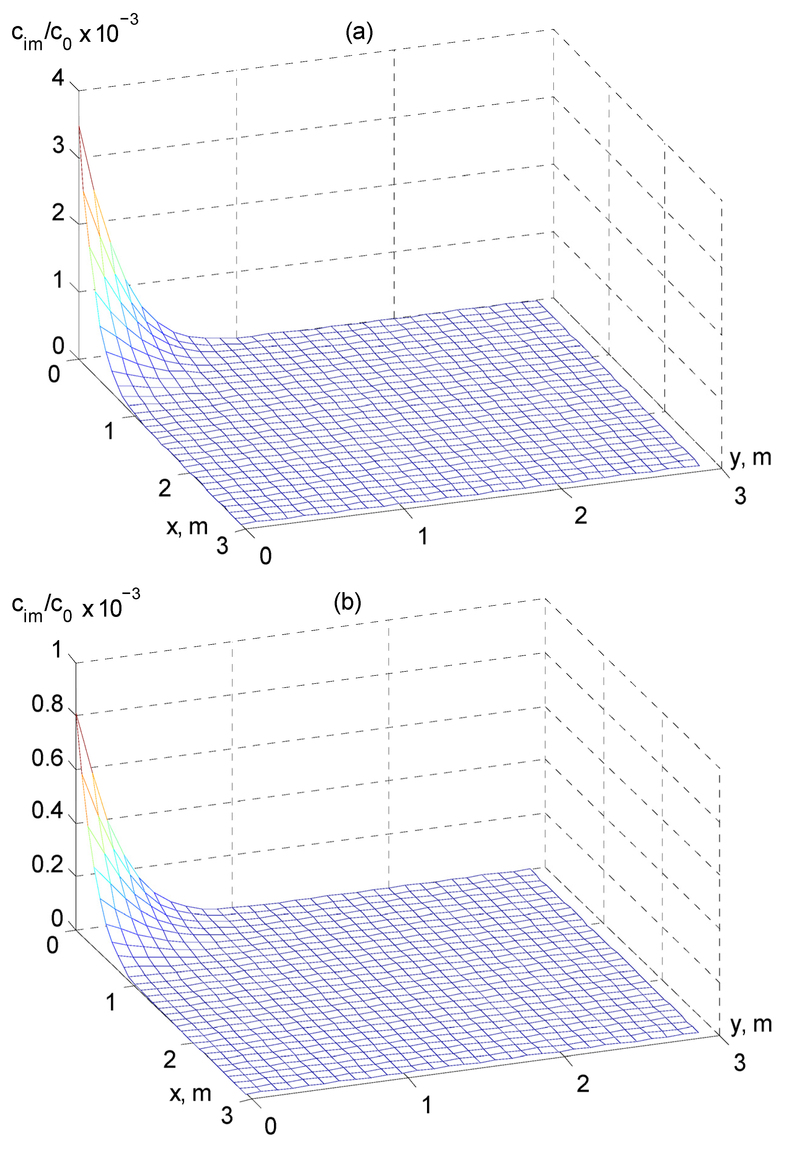
The results of concentration surfaces $c_m$ and $c_{im}$ at $\mathrm{\beta }=2$, ${\mathrm{\delta }}_1=1$, ${\mathrm{\delta }}_2=1,$$t=2400$ s are shown in Figure 4 and Figure 5 for fixed values of $\mathrm{\alpha }=1$, $\mathrm{\alpha }=0.8$, and $\mathrm{\alpha }=0.6$. In these figures, the results show that the decreasing of $\mathrm{\alpha }$ leads to a slowdown in the spread solute distribution in the zone $c_{im}$. The order of the derivative reflects some anomalous conditions in this zone, such as the presence of obstacles, changes in the physical properties of the media, or the influence of external factors.

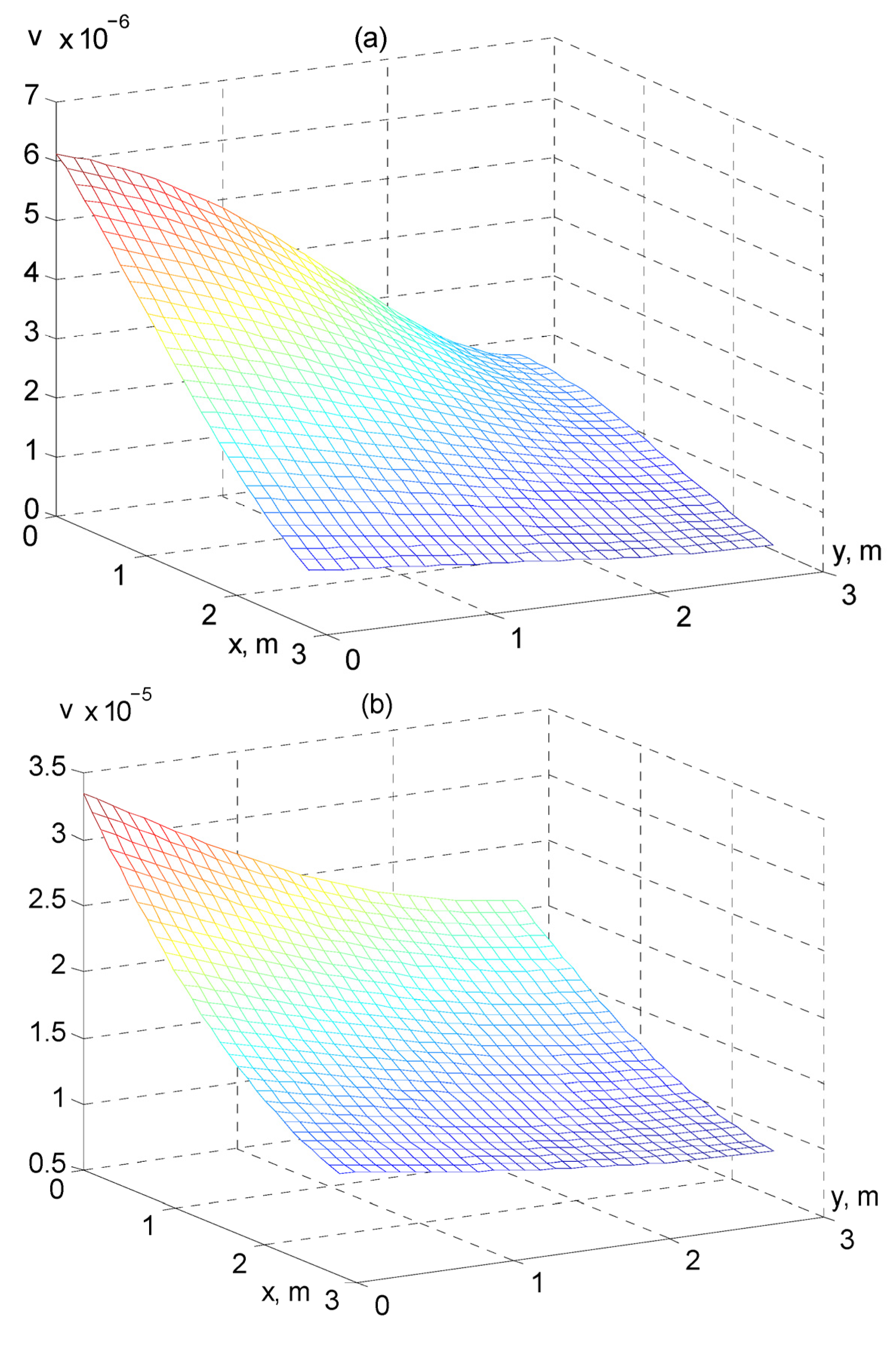
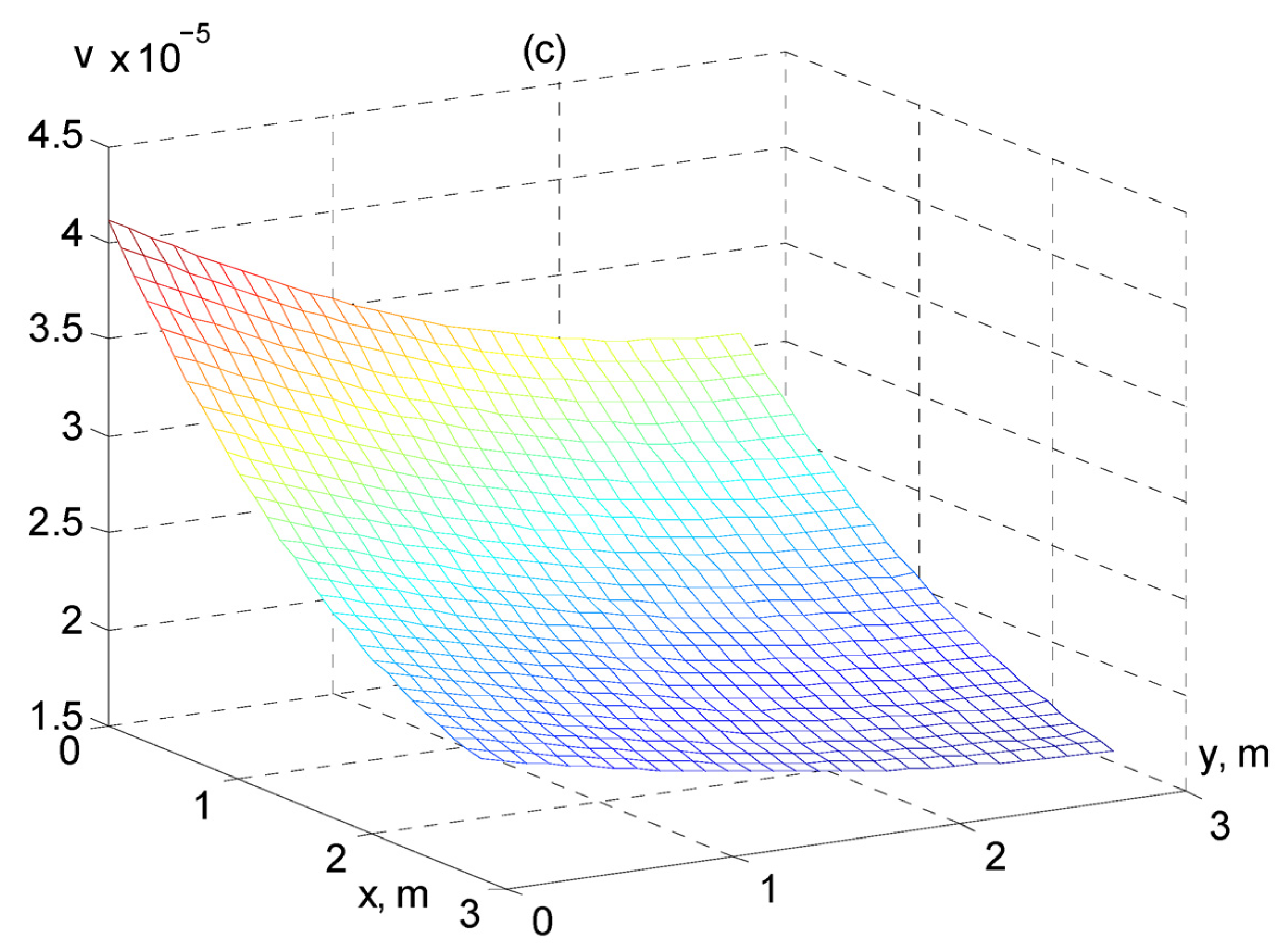
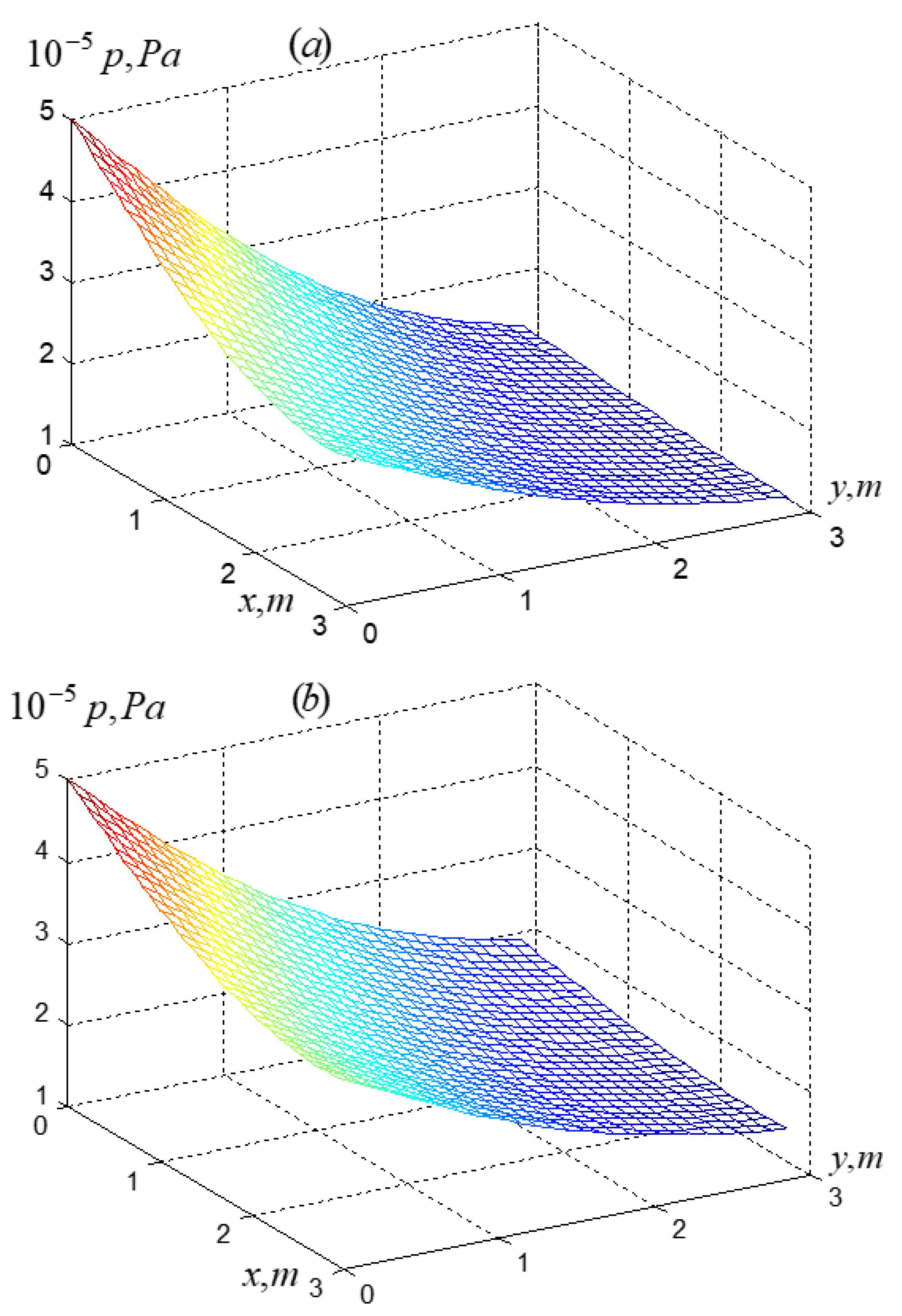
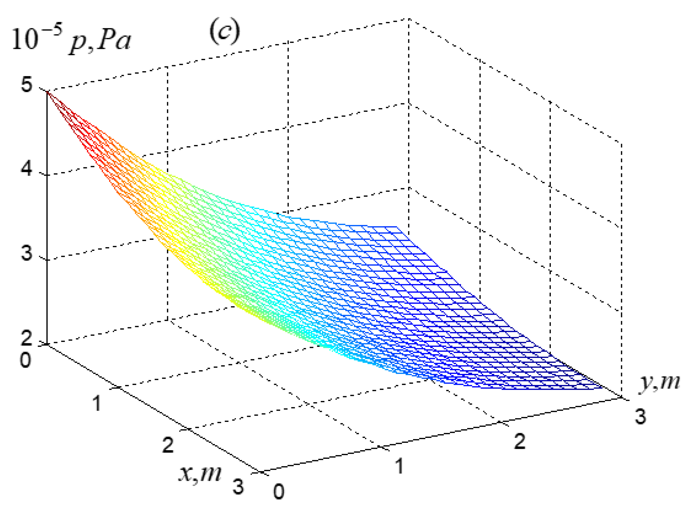
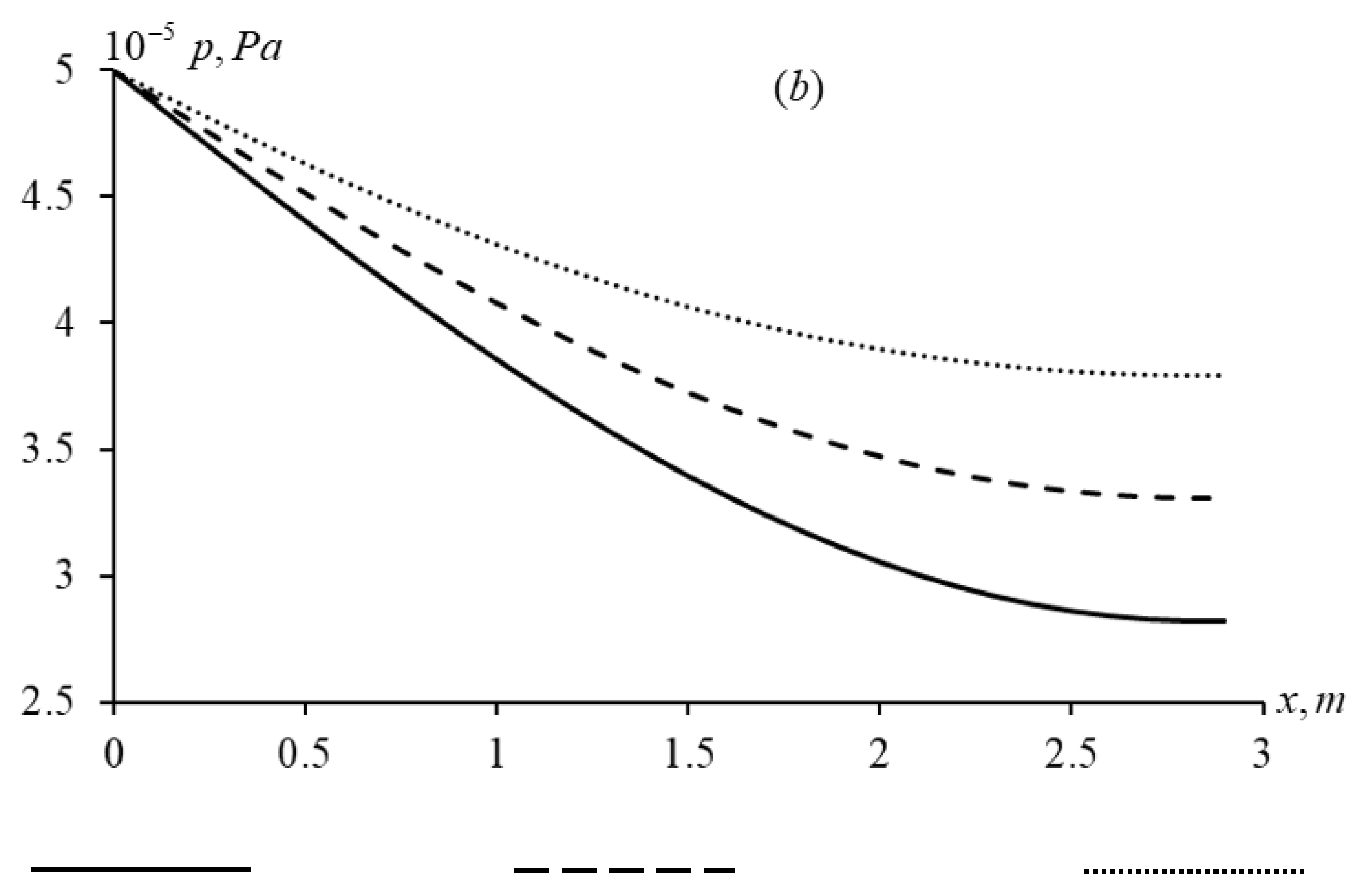
The velocity and pressure profiles at $\mathrm{\alpha }=1$, $\mathrm{\beta }=2$, $t=2400$ s are depicted in Figure 6 and Figure 7. The results are analysed for ${\mathrm{\delta }}_1=1$, ${\mathrm{\delta }}_2=1$ (Figure 6a and Figure 7a) ${\mathrm{\delta }}_1=0.8$, ${\mathrm{\delta }}_2=0.8$ (Figure 6b and Figure 7b) and ${\mathrm{\delta }}_1=0.6$, ${\mathrm{\delta }}_2=0.6$ (Figure 6c and Figure 7c). A decrease in the order of derivatives in piezoconductivity equations ${\mathrm{\delta }}_1$ and ${\mathrm{\delta }}_2$ from the value 1 leads to an increase in pressure and velocity. The system becomes less sensitive to changes in the pressure gradient, which in turn leads to an increase in pressure and filtration velocity when the order of the derivative decreases.

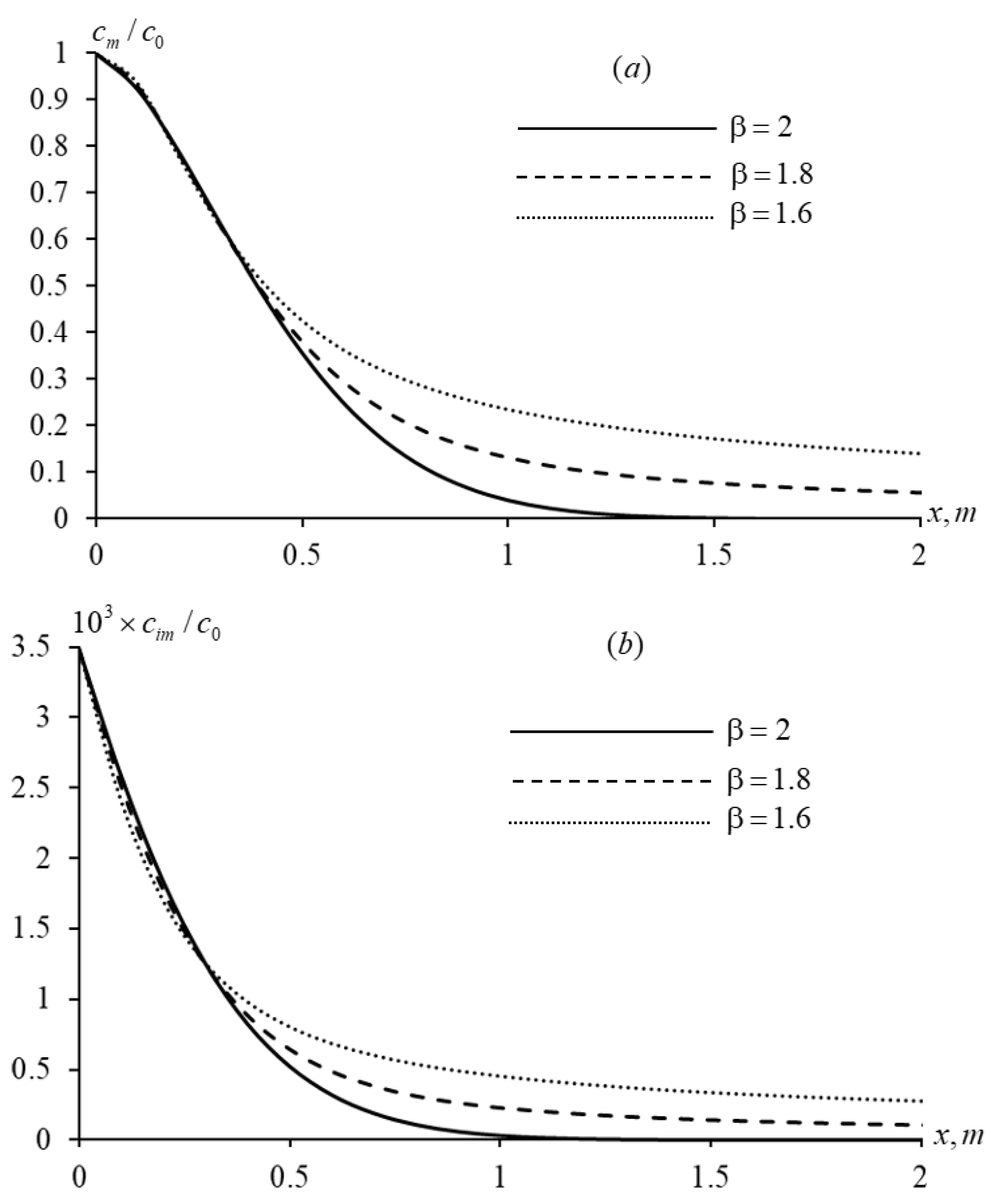
It can be seen from Figure 8a,b that a decrease in the order of derivatives $\mathrm{\beta }$ leads to a more intensive distribution of the concentration field $c_m$. This corresponds to the case of “fast diffusion”. This concentration distribution in the macropore is also reflected in the distribution of the micropore (Figure 8b). To get a clear understanding of the solute concentration distributions $c_m/c_0$ and $c_{im}/c_0$ on the basis of Figure 2 and Figure 3, their profiles were depicted at a given cross-section $y=0$ for a given $t$ and different $\mathrm{\beta }$ (Figure 8).

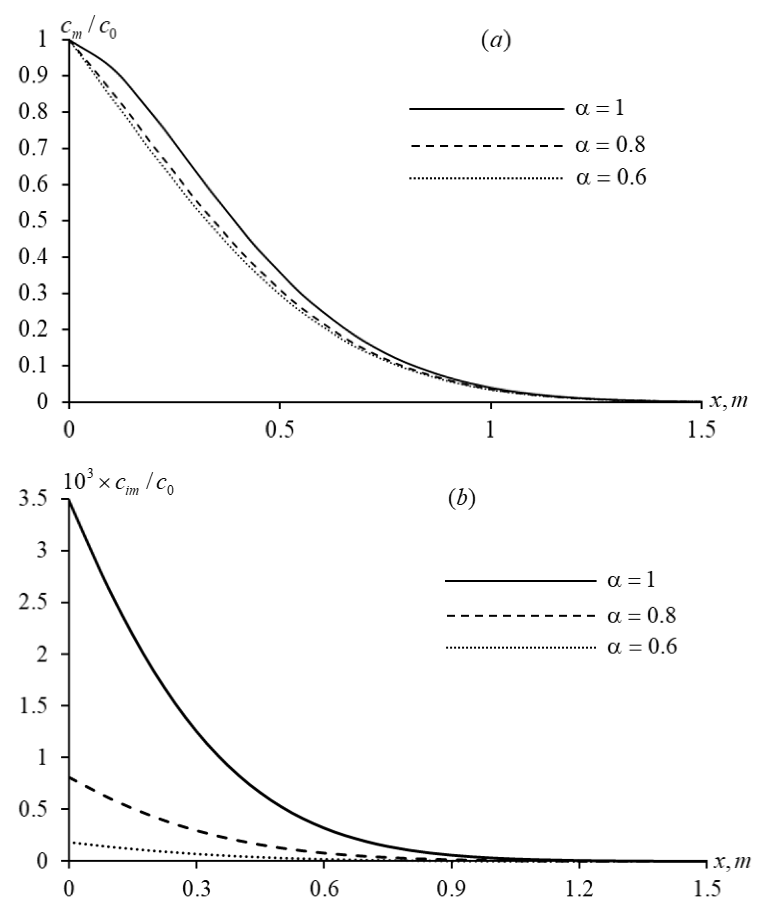
Based on Figure 4 and Figure 5, their profiles were plotted at a given cross-section $y=0$ for a given $t$ and different $\mathrm{\alpha }$ (Figure 9) in order to get a clear understanding of the solute concentration distributions, $c_m/c_0$ and $c_{im}/c_0$. From Figure 9, it can be seen that when the derivative order $\mathrm{\alpha }$ in the kinetic equation decreases from 1, the concentration profiles show slow distributions in both zones $c_m$ and $c_{im}$, which leads to “slow diffusion”.

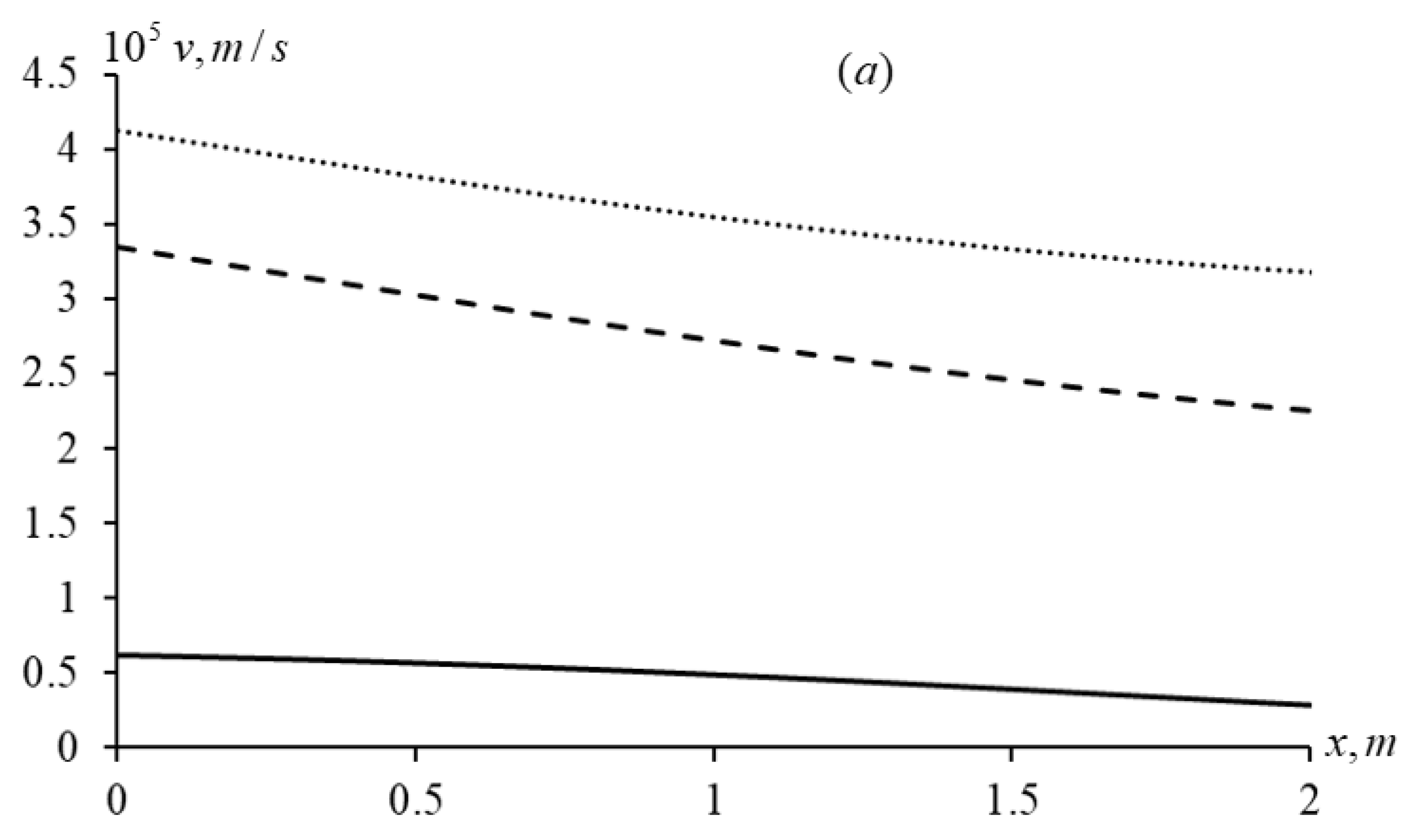
Figure 10 shows cross-sections of the filtration velocity and pressure fields in Figure 6 and Figure 7, respectively. It can be seen from Figure 10 that decreasing the orders of the derivative in the anomalous filtration equation, ${\mathrm{\delta }}_1$ and ${\mathrm{\delta }}_2,$ from 1 leads to an increase in pressure and filtration velocity distribution.

4. Conclusions

An anomalous filtration and solute transport problem is investigated for a two-dimensional porous medium characterised by a fractal structure. The medium is assumed to consist of two interacting regions: one containing mobile fluid and the other containing immobile fluid. These regions are not physically separated in space; rather, both are assumed to coexist at every point within the porous domain. In the mobile-fluid region, fluid flow is governed by an anomalous piezoconductivity equation, while solute transport is described using an anomalous convection–diffusion equation. A boundary-value problem is formulated in which fluid containing solute is injected at a specified boundary point, and the resulting system is solved numerically. Fractional derivatives appearing in the model are interpreted in the sense of Caputo. The numerical results indicate that reducing the spatial fractional derivative order from 2 enhances the diffusion rate, leading to fast-diffusion behaviour. Conversely, decreasing the order of the time-fractional derivative, from 1 in the kinetic equation governing the immobile-fluid region, causes a slowdown of the diffusion process. A reduction in the fractional order within the filtration equation results in higher pressure values and increased filtration velocity. The study demonstrates that solute transport characteristics in both regions are primarily influenced by the concentration distribution within the macropore space, along with other governing hydrodynamic parameters. This model may be beneficial to the treatment process in oil reservoirs.

References

1. Van Genuchten, M.T.; Wierenga, P.J. Mass transfer studies in sorbing porous media I. Analytical solutions. Soil Sci. Soc. Am. J. 1976, 40, 473–480. [Google Scholar] [CrossRef] [Scilit]
2. Makhmudov, J.M.; Usmonov, A.I.; Kuljanov, J.B. Problem of anomalous filtration in nonhomogeneous porous medium. Int. J. Appl. Math. 2023, 36, 189–203. [Google Scholar]
3. Izmerov, M.A.; Tikhomirov, V.P. Filtration model of flow through a fractal porous medium. Fundam. Appl. Probab. Eng. Technol. 2014, 3, 7–14. [Google Scholar]
4. Tikhomirov, V.P.; Gorlenko, O.A.; Izmerov, M.A. Flow through a fractal porous medium. News Samara Sci. Cent. Russ. Acad. Sci. 2011, 13, 879–883. [Google Scholar]
5. Błasik, M. The Implicit Numerical Method for the Radial Anomalous Sub Diffusion Equation. Symmetry 2023, 15, 1642. [Google Scholar]
6. Marasi, H.R.; Derakhshan, M.H. Numerical simulation of time variable fractional order mobile–immobile advection–dispersion model based on an efficient hybrid numerical method with stability and convergence analysis. Math. Comput. Simul. 2023, 205, 368–389. [Google Scholar]
7. Van Genuchten, M.T.; Wagenet, R.J. Two-site/two-region models for pesticide transport and degradation: Theoretical development and analytical solutions. Soil Sci. Soc. Am. J. 1989, 53, 1303–1310. [Google Scholar]
8. Sharma, P.K.; Shukla, S.K.; Choudhary, R.; Swami, D. Modeling for solute transport in mobile–immobile soil column experiment. ISH J. Hydraul. Eng. 2016, 22, 204–211. [Google Scholar]
9. Ding, X.-H.; Luo, B.; Zhou, H.-T.; Chen, Y.-H. Generalized solutions for advection–dispersion transport equations subject to time- and space-dependent internal and boundary sources. Comput. Geotech. 2025, 178, 106944. [Google Scholar]
10. Li, G.; Sun, C.; Jia, X.; Du, D. Numerical solution to the multi-term time fractional diffusion equation in a finite domain. Numer. Math. Theor. Meth. Appl. 2016, 9, 337–357. [Google Scholar]
11. Khuzhayorov, B.; Usmonov, A.; Long, N.N.; Fayziev, B. Anomalous solute transport in a cylindrical two-zone medium with fractal structure. Appl. Sci. 2020, 10, 5349. [Google Scholar]
12. Djordjevich, A.; Savovic, S.; Janicijevic, A. Explicit finite-difference solution of two-dimensional solute transport with periodic flow in homogeneous porous media. J. Hydrol. Hydromech. 2017, 65, 426–432. [Google Scholar]
13. Ngondiep, E. A two-level factored Crank–Nicolson method for two-dimensional nonstationary advection-diffusion equation with time dependent dispersion coefficients and source terms. Adv. Appl. Math. Mech. 2021, 13, 1005–1026. [Google Scholar]
14. Lindstrom, F.T.; Boersma, L. Analytical solutions for convective-dispersive transport in confined aquifers with different initial and boundary conditions. Water Resour. Res. 1989, 15, 241–256. [Google Scholar]
15. Guerrero, J.S.P.; Pimentel, L.C.G.; Skaggs, T.H. Analytical solution of the advection–dispersion transport equation in layered media. Int. J. Heat Mass Transf. 2013, 56, 274–282. [Google Scholar]
16. Ciftci, E.; Avci, C.B.; Borekci, O.S.; Sahin, A.U. Assessment of advective–dispersive contaminant transport in heterogeneous aquifers using a meshless method. Environ. Earth Sci. 2012, 67, 2399–2409. [Google Scholar]
17. Anley, E.F.; Sun, C. Numerical solution of two-dimensional nonlinear time–space fractional reaction advection–diffusion equation with its application. Int. J. Appl. Comput. Math. 2025, 11, 60. [Google Scholar]
18. Savovic, S.; Djordjevich, A. Finite difference solution of the one-dimensional advection diffusion equation with variable coefficients in semi-infinite media. Int. J. Heat Mass Transf. 2012, 55, 4291–4294. [Google Scholar]
19. Savovic, S.; Djordjevich, A. Numerical solution for temporally and spatially dependent solute dispersion of pulse type input concentration in semi-infinite media. Int. J. Heat Mass Transf. 2013, 60, 291–295. [Google Scholar]
20. Yadav, R.R.; Kumar, L.K. Two-dimensional conservative solute transport with temporal and scale-dependent dispersion: Analytical solution. Int. J. Adv. Math. 2018, 2, 90–111. [Google Scholar]
21. Khuzhayorov, B.K.; Viswanathan, K.K.; Kholliev, F.B.; Usmonov, A.I. Anomalous Solute Transport Using Adsorption Effects and the Degradation of Solute. Computation 2023, 11, 229. [Google Scholar] [CrossRef] [Scilit]
22. Sweilam, N.H.; Ahmed, S.M.; Adel, M. A simple numerical method for two-dimensional nonlinear fractional anomalous sub-diffusion equations. Math. Methods Appl. Sci. 2021, 44, 2914–2933. [Google Scholar]
23. Salomoni, V.A.L.; De Marchi, N. Numerical solutions of space-fractional advection–diffusion–reaction equations. Fractal Fract. 2021, 6, 21. [Google Scholar]
24. Samarskii, A.A. The Theory of Difference Schemes; CRC Press: Boca Raton, FL, USA, 2001. [Google Scholar]
Figure 1. Scheme of solute transport in a two-zone medium.
Computation 14 00090 g001
Figure 2. Surfaces of relative concentration c m / c 0 for α = 1 , δ 1 = 1 , δ 2 = 1 , t = 2400 sat different values of β : (a) β = 2 , (b) β = 1.8 , (c) β = 1.6 .
Computation 14 00090 g002aComputation 14 00090 g002b
Figure 3. Surfaces of relative concentration c i m / c 0 for α = 1 , δ 1 = 1 , δ 2 = 1 , t = 2400 sat different values of β : (a) β = 2 , (b) β = 1.8 , (c) β = 1.6 .
Computation 14 00090 g003aComputation 14 00090 g003b
Figure 4. Surfaces of relative concentration c m / c 0 for β = 2 , δ 1 = 1 , δ 2 = 1 , t = 2400 sat different values of (a) α = 1 , (b) α = 0.8 , (c) α = 0.6 .
Computation 14 00090 g004aComputation 14 00090 g004b
Figure 5. Surfaces of relative concentration c i m / c 0 for β = 2 , δ 1 = 1 , δ 2 = 1 , t = 2400 sat different values: (a) α = 1 , (b) α = 0.8 , (c) α = 0.6 .
Computation 14 00090 g005aComputation 14 00090 g005b
Figure 6. Surfaces of velocity v at α = 1 , β = 2 , t = 2400 s at different values: (a) δ 1 = 1 , δ 2 = 1 , (b) δ 1 = 0.8 , δ 2 = 0.8 , (c) δ 1 = 0.6 , δ 2 = 0.6 .
Computation 14 00090 g006aComputation 14 00090 g006b
Figure 7. Surfaces of pressure p at α = 1 , β = 2 , t = 2400 s at different values: (a) δ 1 = 1 , δ 2 = 1 , (b) δ 1 = 0.8 , δ 2 = 0.8 , (c) δ 1 = 0.6 , δ 2 = 0.6 .
Computation 14 00090 g007aComputation 14 00090 g007b
Figure 8. Concentration profiles (a) c m / c 0 and (b) c i m / c 0 for α = 1 , δ 1 = 1 , δ 2 = 1 , t = 2400 s at various values of β ; y = 0 . .
Computation 14 00090 g008
Figure 9. Concentration profiles (a) c m / c 0 and (b) c i m / c 0 at β = 2 , δ 1 = 1 , δ 2 = 1 , t = 2400 s at different α ; y = 0 .
Computation 14 00090 g009
Figure 10. Filtration velocity (a) profiles and (b) pressure fields for α = 1 , β = 2 , t = 2400   s at various values of δ 1 , δ 2 ; y = 0 . Computation 14 00090 i001   δ 1 = 1 , δ 2 = 1 ; Computation 14 00090 i002   δ 1 = 0.8 , δ 2 = 0.8 ; Computation 14 00090 i003   δ 1 = 0.6 , δ 2 = 0.6 .
Computation 14 00090 g010aComputation 14 00090 g010b
Disclaimer/Publisher’s Note: The statements, opinions and data contained in all publications are solely those of the individual author(s) and contributor(s) and not of MDPI and/or the editor(s). MDPI and/or the editor(s) disclaim responsibility for any injury to people or property resulting from any ideas, methods, instructions or products referred to in the content.