SPL-Based Modeling of Serrated Airfoil Noise via Functional Regression and Ensemble Learning

Abstract

This study presents a semi-empirical approach to generalizing the acoustic radiation generated by serrated airfoil configurations, based on small-scale aerodynamic/acoustic experiments and functional regression techniques. In the context of passive noise reduction strategies, such as leading-edge and trailing-edge serrations, acoustic measurements are performed in a controlled subsonic wind tunnel environment. Sound pressure level (SPL) spectra and acoustic power metrics are acquired for various geometric configurations and flow conditions. These spectral data are then analyzed using regression-based modeling techniques—linear, quadratic, logarithmic, and exponential forms—to capture the dependence of acoustic emission on key geometric and flow-related variables (e.g., serration amplitude, wavelength, angle of attack), without relying explicitly on predefined nondimensional numbers. The resulting predictive models aim to describe SPL behavior across relevant frequency bands (e.g., broadband or 1/3 octave) and to extrapolate acoustic trends for configurations beyond those tested. The proposed methodology allows for the identification of compact functional relationships between configuration parameters and acoustic output, offering a practical tool for the preliminary design and optimization of low-noise serrated profiles. The findings are intended to support both physical understanding and engineering application, bridging experimental data and parametric acoustic modeling in aerodynamic noise control.

1. Introduction

The generation and control of aerodynamic noise remains a major challenge in the design of modern aerodynamic systems operating at low-to-moderate Mach numbers. In particular, noise originating from the interaction of turbulent flow structures with the solid boundaries of lifting surfaces continues to be a key focus in aeroacoustic research [1,2]. This interaction-type noise mechanism is especially critical in open-rotor configurations, wind turbines, and manned and unmanned aerial vehicles (UAVs), where passive control methods are desirable due to weight, power, and robustness constraints [3,4,5,6,7,8].

Trailing-edge (TE) and leading-edge (LE) serrations have emerged as effective passive devices for broadband noise reduction, acting primarily by modifying the turbulent pressure fluctuations near surface discontinuities [9,10]. Their ability to reduce far-field sound levels without compromising aerodynamic performance has motivated extensive experimental and theoretical investigations over the last two decades [11,12]. Serrations with sinusoidal, triangular, and hybrid geometries have been tested in a variety of configurations, highlighting the role of geometrical parameters such as amplitude (h), wavelength (λ), and skewness in controlling noise generation [13,14,15,16,17,18].

Foundational theoretical models, including Howe’s surface pressure scattering formulation [19], Amiet’s trailing-edge theory for turbulent boundary layer noise [20], and the empirical framework of Brooks, Pope, and Marcolini [21], have provided the basis for understanding the mechanisms of serration-induced acoustic attenuation [22]. However, these models often rely on simplified flow assumptions, such as frozen turbulence and idealized boundary conditions, which limit their applicability to complex geometries and flow scenarios [15,23,24]. Traditional theoretical and numerical models for serrated airfoil noise often require complex flow simulations and rely on pre-calibrated dimensionless numbers. These methods, while informative, may lack generality across configurations. Therefore, a semi-empirical and regression-based strategy is adopted in this work, aiming to exploit experimental data to capture acoustic behavior using interpretable and tunable expressions.

To complement these models, recent studies have focused on obtaining experimental acoustic spectra for serrated configurations under controlled flow conditions. These measurements frequently reveal broadband attenuation patterns that are difficult to generalize using classical theory alone [3,12,25]. As a result, semi-empirical and data-driven models have been proposed to approximate the observed SPL behavior across frequency bands using functional relationships with geometric and flow variables [26].

Several of these models may rely on regression techniques—linear, quadratic, logarithmic, or exponential—to link changes in SPL or OASPL to parameters such as serration amplitude, spacing, angle of attack, or velocity. For instance, one commonly used form expresses the attenuation as a logarithmic function of the normalized serration geometry, for example, derived from idealized triangular serration profiles. Other formulations rely on polynomial fits or exponential decay terms to capture spectral trends across frequency. In several cases, the adopted functions are fitted pointwise across frequency bins or integrated over predefined bands, depending on the availability and granularity of the acoustic data. Previous studies have explored regression techniques based on dimensionless groups or flow parameters (detailed in the following section). However, these are often limited in scope or rely on predefined scaling laws. The present study differs by directly linking SPL with raw experimental parameters and assessing multiple regression types, including polynomial, exponential, and Random Forest models. While analytical derivations remain relevant for simplified geometries, such as [27], many recent approaches emphasize regression-based surrogate models trained on experimental datasets [11,26]. Polynomial surface fitting can be used to approximate broadband noise attenuation based on serration amplitude and wavelength, while exponential decay models are suitable for frequency-resolved regression. Design variables such as skewness or local angle of attack may also be incorporated into extended formulations through second-order or interaction terms. These approximations are typically embedded within reduced-order frameworks and are suited for interpolation across experimental configurations or limited extrapolation within validated bounds. Some formulations, such as those in [15,28], explicitly target integration into computational workflows, offering closed-form expressions or spectral templates calibrated from wind tunnel data.

Despite these advances, most models remain application-specific and depend strongly on geometry, flow regime, and the spectral resolution of the experimental data. This motivates the development of generalizable, semi-empirical frameworks capable of capturing the influence of geometric and aerodynamic conditions on noise generation, without relying solely on first principles or high-fidelity simulations. In this context, the present work aims to construct predictive models of SPL and acoustic power spectra using regression-based fitting applied to experimental data obtained at a reduced scale. The methodology integrates physical insight from classical theory with empirical flexibility, enabling compact expressions that relate acoustic output to measurable design variables. The SPL induced by serrated airfoil edges is influenced not only by the geometric features of the serration but also by trailing-edge self-noise mechanisms, which originate from turbulence–structure interactions. The objective of this study is to develop and validate a data-driven framework to model the sound pressure level (SPL) generated by serrated leading-edge airfoils, combining functional regression and ensemble learning. This approach aims to capture complex interactions between design and flow variables without relying on predefined similarity numbers, thereby offering more adaptable and generalizable models. Unlike many existing models, which express SPL variations through established nondimensional terms such as Strouhal or Reynolds numbers, the present work introduces formulations directly tied to experimental parameters. This avoids predefined similarity assumptions and enhances model transparency and interpretability.

Existing analytical models for trailing-edge noise, such as BPM or Howe’s theory, often assume idealized boundary layer behavior or rely on global geometric parameters. These limitations make them less suitable for modern serrated designs, where noise generation is influenced by multiple geometric and flow variables in a nonlinear way. Current semi-empirical models, such as the BPM approach, integrate theoretical formulations (e.g., edge scattering) with experimentally calibrated parameters to achieve robust broadband noise predictions [23]. However, these methods are primarily tailored to trailing-edge mechanisms and depend on flow quantities like boundary layer thickness or wall shear stress, which are difficult to extract in complex experimental setups involving serrated leading edges and installation effects. By bridging theory and experiment through functional regression, the present study introduces a modeling framework that avoids the reliance on predefined nondimensional groups, using only measurable geometric and angular descriptors. This strategy contributes to the development of practical design tools for low-noise serrated airfoil configurations, with potential applications in propulsion, energy, and rotorcraft systems. The methodology developed here is intended not only as a diagnostic tool for understanding the acoustic behavior of serrated edges but also as a predictive framework that can support the design of quieter airfoils in both aeroacoustic testing and real-world applications. After introducing the experimental configuration used to capture the acoustic response of serrated leading edges, the second section describes the data processing workflow and the modeling strategies applied, including both functional regression and ensemble-based approaches. This is followed by a detailed analysis of the results, where the predictive performance and physical relevance of the models are critically assessed. Finally, the discussion and conclusions highlight the main findings and their implications for both aeroacoustic research and practical engineering applications.

2. Materials and Methods

The regression-based methods employed in this study are grounded in the need to develop compact, predictive expressions for the acoustic response of serrated airfoil configurations, using datasets obtained at reduced scale. Rather than relying solely on classical theoretical frameworks or computationally intensive simulations, the aim is to approximate sound pressure level (SPL) variations as functions of physically meaningful, experimentally accessible variables. These approximations are built to retain spectral fidelity, with the added benefit of being applicable across geometrically diverse configurations. The dependent variable throughout this study is defined as the difference in SPL (ΔSPL) relative to a baseline configuration, either frequency-resolved or integrated over 1/3-octave bands. The same regression structure can also be applied to other acoustic metrics such as overall sound pressure level (OASPL), sound power level (PWL), or power spectral density (PSD), all of which have been modeled with similar mathematical forms. The independent variables are chosen based on their relevance to both aerodynamic behavior and acoustic scattering potential. The normalized serration amplitude h/λ captures the geometric sharpness and periodicity of the edge. The angle of attack α influences the effective impingement direction of incoming turbulence. The observation angles θ and ϕ reflect the spatial distribution of acoustic radiation, while the number of teeth N encodes the serration density. All variables are nondimensionalized to ensure generalizability and eliminate scale dependency. To capture the relationship between ΔSPL and these parameters, four families of regression models were considered. These functional forms were selected to cover both linear trends and nonlinear saturation behaviors observed in prior experimental studies [29]. The general equations are formulated from linear (1), polynomial (2), logarithmic (3) to exponential (4) as functional forms used for regression modeling of acoustic metrics (ΔSPL, OASPL, PWL, PSD).

$$y=a_0+\sum a_i{x}_i$$

(1)

$$y=a_0+a_1{x}_1+a_2{x}_1^2+\dots +a_n{x}_n^k$$

(2)

$$y=a_0+a_1\mathit{log}\left(x_1\right)+a_2{x}_2+\dots$$

(3)

$$y=a_0+a_1{e}^{-a_2{x}_1}+a_3{x}_2+\dots$$

(4)

To explore the relationship between acoustic output and governing parameters (serration geometry, angular installation, observation angles), several regression models were tested, as in Equations (1)–(4). Each formulation was selected based on its ability to capture specific behaviors observed in the SPL datasets. Linear models (Equation (1)) provide a baseline reference, assuming additive and proportional relationships between variables such as NT (number of teeth), α (installation angle), or observer direction. Although conceptually simple, this approach can underfit in cases where the acoustic response exhibits curvature or directional peaks. Polynomial regressions (Equation (2)), ranging from second to fourth order, were therefore employed to capture nonlinear dependencies—particularly useful in modeling angular directivity or identifying local extrema in SPL distributions. Their flexibility makes them effective in fitting wide-aperture beam patterns or identifying geometric thresholds in noise reduction. Logarithmic models (Equation (3)) were introduced given the prevalence of log-scaled representations in acoustic theory (e.g., SPL itself), and the observation that some input variables, such as NT or observer angle, produced diminishing returns on SPL variation—consistent with log-behavior. Exponential models (Equation (4)) were motivated by the decay patterns often encountered in frequency-dependent propagation losses or wake-induced acoustic attenuation. These also proved useful in scenarios where small variations in certain predictors (e.g., Strouhal-based proxies or relative elevation) resulted in disproportionately large SPL responses.

In addition to these analytical forms, ensemble learning was explored via Random Forest regression, due to its capacity to handle nonlinear interactions without prior assumptions about functional structure. This data-driven method captured complex directional effects and high-dimensional interactions, although at the cost of interpretability. All models used the same input predictors, namely the geometric and angular parameters (e.g., NT, α, φ, θ), while the targets were either global SPL metrics (OASPL) or spatially resolved values over the measurement grid. The performance of each model was primarily evaluated using the coefficient of determination (R²), which balances fit quality with model complexity and offers a robust measure of how well the regression captures the main acoustic trends observed in the SPL data. Given the high signal consistency (80–100 dB range) and minimal background noise, R² remains the most suitable indicator in this context. For benchmarking purposes, additional metrics such as RMSE (Root Mean Square Error) and MAE (Mean Absolute Error) will also be computed for representative configurations, as they offer complementary views by quantifying absolute and average prediction errors in decibels.

These forms are not purely theoretical: similar functional dependencies have been identified in experimental studies on serrated edges. Pereira et al. [17] reported a logarithmic relationship between ΔSPL and the normalized wavelength parameter 2 h/λ, showing saturation behavior beyond a certain threshold. Their model, ΔSPLₘₐₓ = 10 log₁₀[1 + 4 (2 h/λ)²], mirrors Equation (3) and supports the use of such approximations in regression. A more detailed logarithmic formulation for SPL has been identified in [29]. In the case of acoustic power, the relationship between OASPL and directivity is described in [30] through a model incorporating both trigonometric and logarithmic terms. Additional formulations are referenced in [31], particularly those addressing trailing-edge noise arising from boundary layer separation. Lee et al. [3] proposed a combined log-polynomial expression to describe narrowband SPL contributions in rotor experiments:

$$SPL\left(f\right)={\displaystyle \frac{f_0{∆}^{0.6}}{{\left[f_3{∆}^{f_4}+f_5\right]}^{f_6}+{\left[f_7∆\right]}^{f_8}}}$$

(5)

where f₀ … f₈ may depend on variables such as f, Mt, Vt, and St in various combinations (linear to log).

Further, Gruber et al. [9] demonstrated that noise reduction effects depend critically on both h/δ and a Strouhal-based scaling St_δ = fδ/U. In such cases, exponential or log-based models better capture threshold or plateau behavior observed experimentally. A combined approach in the acoustic domain—addressing both transmission and absorption losses—based on logarithmic functions and quadratic terms, is presented in [32]. Comparable approaches are applied in modeling OASPL and PWL trends, particularly when correlating acoustic output with Reynolds or Strouhal numbers, as shown in parametric investigations [33], where the SPL associated with Tip Vortex Formation Noise (TVFN) is expressed as a function of empirical constants, observer location, Mach number, and Strouhal number. In the broader context of blade-related noise sources, Küçükosman [34] provides a comprehensive synthesis of wall-pressure spectrum models, showing that—depending on the chosen formulation (e.g., Goody, Rozenberg, Catlett, Hu)—the spectral behavior is driven by different flow parameters and boundary layer characteristics.

From a broader perspective, experimental trends identified in the literature consistently highlight the dependence of key acoustic quantities on flow and geometric parameters. Linear variations of ΔSPL are often observed with respect to serration geometry parameters such as the amplitude-to-wavelength ratio h/λ, installation angle α, serration count N, and observer elevation ϕ. Polynomial relationships have been reported for the spectral behavior of SPL as a function of frequency, while OASPL shows parametric dependencies on tip Mach number M_tip, observer angle θ, and frequency f. Logarithmic trends are noted for ΔSPL and PWL with respect to serration ratio 2 h/λ, Strouhal number (St), and Reynolds number (Re). 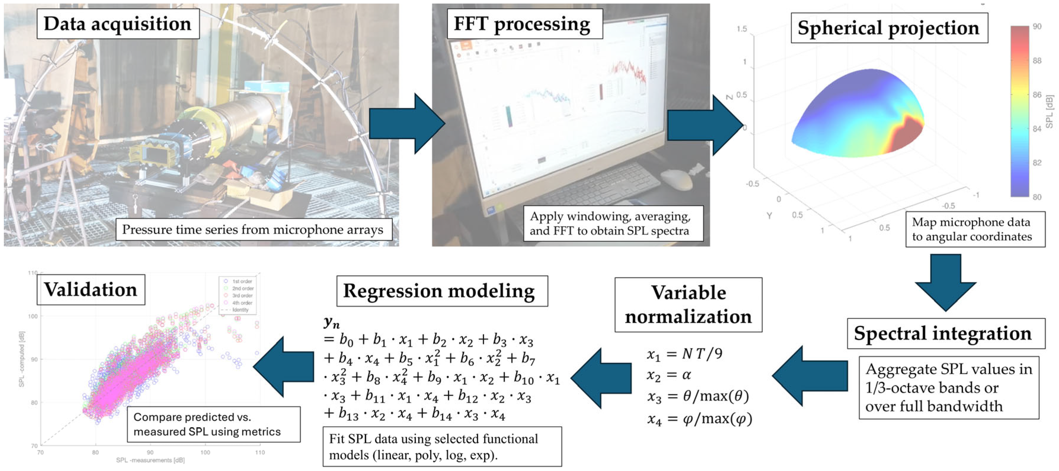Additionally, exponential dependencies have been proposed to describe OASPL and Power Spectral Density (PSD) variations as a function of normalized Strouhal parameters such as St_δ and relative serration amplitude h/δ. These correspondences highlight the growing prevalence of compact regression-based models in experimental aeroacoustics, especially for describing the influence of geometric and flow-related variables on sound generation. The structure and parametrization employed here are thus both practical and supported by a solid experimental foundation. In order to establish such a functional relationship, the analytical process outlined in Figure 1 is adopted, guiding the transition from raw acoustic data to regression-based parametric laws.

To assess the statistical relevance of each independent variable (serration count, angle of attack, observation angle θ, and elevation φ) on the resulting SPL levels, a one-way analysis of variance (ANOVA) was employed. This method evaluates whether the mean response differs significantly across levels of each categorical predictor. The normalized data were grouped into discrete bins (0.1 resolution), and the p-values were computed for each variable. Furthermore, effect sizes were quantified using eta squared (η²), indicating the proportion of variance in SPL attributable to each factor. A significance threshold of p < 0.01 was considered strong evidence against the null hypothesis (i.e., no influence).

In addition to the semi-empirical modeling strategy, this study further explores the potential of data-driven regression approaches to approximate the sound pressure level (SPL) generated by serrated leading-edge geometries under varying installation and observation conditions. To this end, a Random Forest (RF) ensemble regression technique was employed, focusing on predictive accuracy and the relative importance of key input variables across multiple subset configurations.

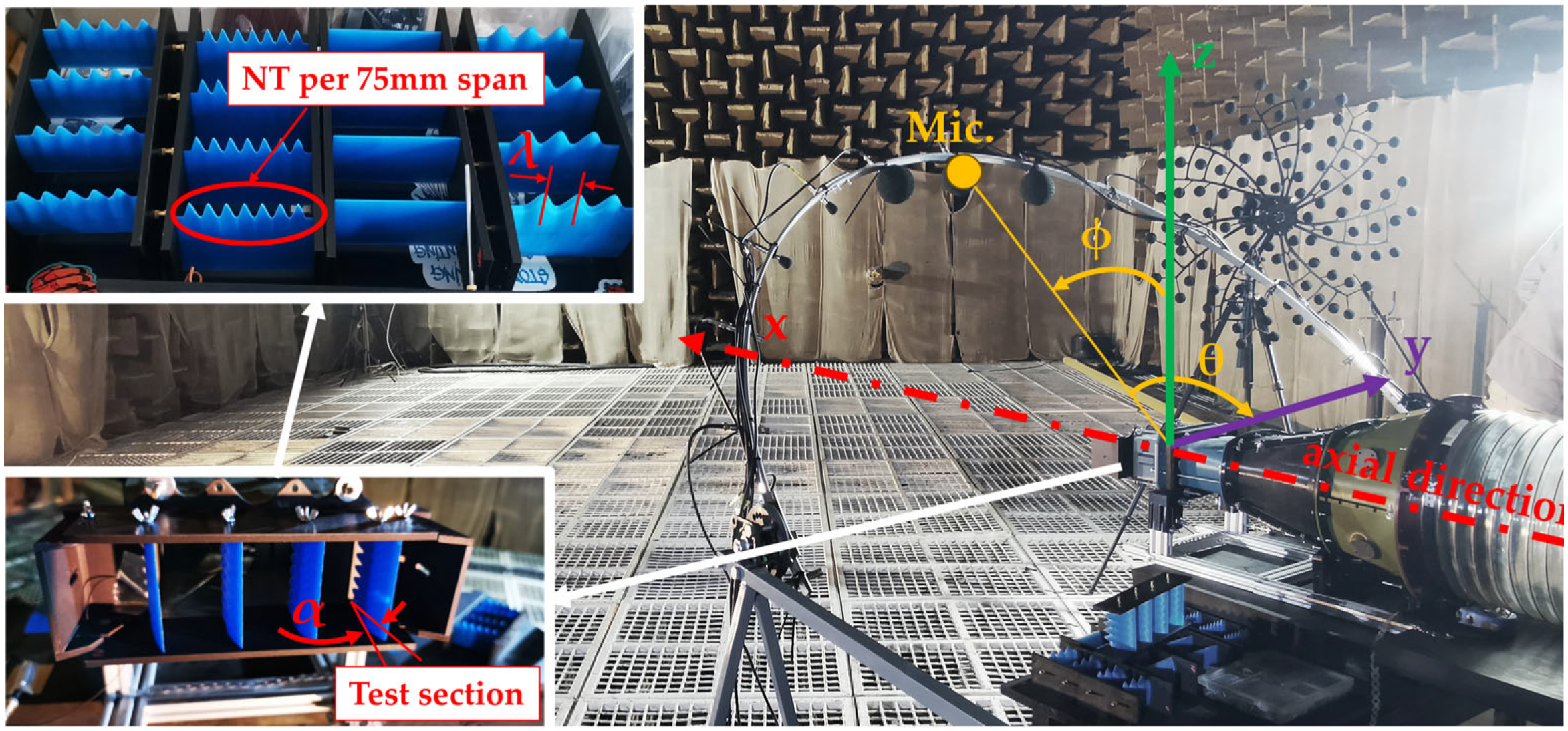
The SPL datasets were obtained from microphone measurements distributed along circular arcs in multiple inclined planes, covering 13 discrete azimuthal positions (θ) and 6 elevation angles (ϕ) explicitly shown in Figure 2. The experimental campaign systematically varied two key geometric parameters: the serration configuration, defined by the number of teeth (NT = 0, 3, 5, 7, 9), and the installation angle (α = 0°, 5°, 10°, 15°), resulting in 20 distinct test cases. Each configuration thus captures the combined influence of serration geometry, angle of attack, and observation direction. The SPL values for each test case were organized into CSV matrices of 6 elevation by 13 azimuth samples. The array consists of 13 GRAS 40 AE microphones equally distanced across 180 degrees connected to two SIRIUS Modular Data Acquisition (DAQ) Systems (8 channels) mounted in series. The experimental setup was coupled to a 9800 Pa, 7.5 kW centrifugal fan (SODECA CA-172-2T-10 IE3, Spain) via a 315 mm diameter corrugated tube that provided in the 125 mm × 75 mm test section a ~50 m/s airflow and a turbulence characteristic length of ~5 mm (by integrating a grid in the convergent area) [35]. The whole setup was placed in the anechoic chamber (1200 m³, 15 × 10 × 8 m) designed and executed according to ISO3745 [36] requirements, with a wall absorption coefficient of 99%, in the 150–20,000 Hz frequency range.

To address potential concerns regarding floor-borne vibrations or mechanical coupling within the anechoic chamber, it is important to note that the microphone array was mechanically decoupled from the aeroacoustic test setup. Specifically, the microphones were mounted on an independent semicircular arc, which rested on metallic floor grids that were not physically connected to the support platform of the air supply system or to the flat plate with serrations. These floor panels were structurally disjoint, preventing mechanical transmission of vibrations between the measurement apparatus and the source assembly. Additionally, to minimize the influence of local aerodynamic disturbances—particularly in the region influenced by the jet—microphones located near the flow path were covered with porous foam. This treatment mitigated high-frequency turbulence-induced fluctuations without introducing acoustic reflections. While no additional signal filtering was applied beyond standard FFT windowing (Hanning), no tonal artifacts, whistling, or low-frequency hums were observed in the raw data that would have necessitated further preprocessing.

In the data preprocessing step, each combination of NT, alpha, theta, and phi was normalized: the number of teeth was scaled by 9, while angular variables were converted to radians and normalized to [0, 1]. From each test file, values corresponding to elevation planes at 15° and 30° were excluded, motivated by both physical and methodological considerations. At these lower inclination angles, the microphones are positioned closer to the jet axis and directly within the turbulent shear layer, where flow-induced disturbances are stronger and more variable. This can result in locally amplified or irregular SPL values that are less representative of far-field acoustic radiation. In contrast, higher elevation angles (φ = 45–90°) capture more stable directivity patterns with lower susceptibility to near-field interference. From a modeling perspective, including φ = 15° and 30° was found to significantly reduce the goodness of fit for all regression types, likely due to the higher variability and directional asymmetry introduced at those angles. As such, the exclusion was intended to improve both model reliability and physical consistency. The resulting dataset included four normalized independent variables. To evaluate the effect of different modeling assumptions, eight data variants were constructed:

• Variant A used all four normalized input variables (NT, α, θ, ϕ).
• Variant B used a reduced set of variables (NT, α, ϕ) and included their pairwise linear interactions.
• Variants C through H explored selective restrictions over NT, α, θ, and ϕ to assess potential increases in regression performance for simplified or constrained physical configurations.

All variants were evaluated using Random Forest-style bootstrapped linear regression, with resampled models. For each tree, regression coefficients were obtained using least-squares fitting (or pseudoinverse when necessary), and the ensemble prediction was taken as the average over all trees. Model performance was assessed using the coefficient of determination (R²) calculated against the original target SPL values. Variable importance was computed via permutation methods: each predictor was randomly shuffled, and the resulting drop in R² (ΔR²) was used to quantify its contribution. Unlike typical implementations of Random Forests in platforms such as Python or R, which rely on decision tree ensembles, the present method was developed entirely in GNU Octave (v9.2.0) using custom code (which was run on a Dell Tower (i9-10920X, 32GB RAM, NVIDIA Quadro RTX 4000 8GB, Round Rock, TX, USA). All functional regression and ensemble learning models presented in this study were implemented explicitly in GNU Octave, without relying on external machine learning libraries such as scikit-learn, statsmodels, or TensorFlow. The modeling routines were constructed manually using native octave syntax, closely following the mathematical formulation of each regression type. For example, polynomial regressions (up to fourth order) were solved via closed-form normal equations, equivalent to MATLAB’s polyfit or NumPy’s polyfit in Python. Logarithmic and exponential models were handled through linearization or nonlinear fitting routines built with lsqcurvefit-style logic. Sinusoidal fits mimicked the structure of Fourier components in constrained least-squares form. Even the ensemble learning approach (Random Forest regression) was implemented from scratch, using custom bootstrapping and decision tree splitting rules similar in structure to fitrensemble in MATLAB or RandomForestRegressor in scikit-learn. This fully manual approach ensured transparency and adaptability to the specific structure of the acoustic dataset, while allowing fine control over input normalization, feature selection, and model interpretation. This approach allows fine control over the modeling process and direct access to regression coefficients and variable importance metrics. While it does not replicate the tree-based structure of classic Random Forest algorithms, it retains the core concept of variance reduction through aggregation of multiple learners.

3. Results

The regression models were trained using structured tabular data derived from processed microphone measurements. Each data sample corresponded to a unique combination of four predictors: the number of serration teeth (NT), the installation angle (α), the azimuthal angle (θ), and the elevation angle (ϕ). These input variables were normalized to [0, 1] ranges prior to training. The target variable was the sound pressure level (SPL), extracted from 6 × 13 matrices (elevation × azimuth) for each of the 20 test configurations, and reshaped into column vectors. All data were stored and processed in CSV format, with each row representing a distinct spatial and geometrical configuration. For the processed data, polynomials were obtained using normalized data and then converted to the dimensional form (it was observed that a slightly better numerical stability is obtained, with a higher R² value in the alternative where we worked with almost unit values). Polynomial approximations have the following structure (from 1st to 4th degree, Equations (6)–(9)).

$$y_{n1}=b_0+b_1·x_1+b_2·x_2+b_3·x_3+b_4·x_4$$

(6)

$$\begin{gathered} y_{n2}=b_0+b_1·x_1+b_2·x_2+b_3·x_3+b_4·x_4+b_5·x_1^2+b_6·x_2^2+b_7·x_3^2+b_8·x_4^2+ \\ {b}_9·x_1·x_2+b_{10}·x_1·x_3+b_{11}·x_1·x_4+b_{12}·x_2·x_3+b_{13}·x_2·x_4+b_{14}·x_3·x_4 \end{gathered}$$

(7)

$$y_{n3}=\left[all 2^{nd} \mathrm{d}\mathrm{e}\mathrm{g}\mathrm{r}\mathrm{e}\mathrm{e} \mathrm{t}\mathrm{e}\mathrm{r}\mathrm{m}\mathrm{s}\right]+b_{15}·x_1^3+b_{16}·x_2^3+b_{17}·x_3^3+b_{18}·x_4^3$$

(8)

$$y_{n4}=\left[all 3^{rd} \mathrm{d}\mathrm{e}\mathrm{g}\mathrm{r}\mathrm{e}\mathrm{e} \mathrm{t}\mathrm{e}\mathrm{r}\mathrm{m}\mathrm{s}\right]+b_{19}·x_1^4+b_{20}·x_2^4+b_{21}·x_3^4+b_{22}·x_4^4$$

(9)

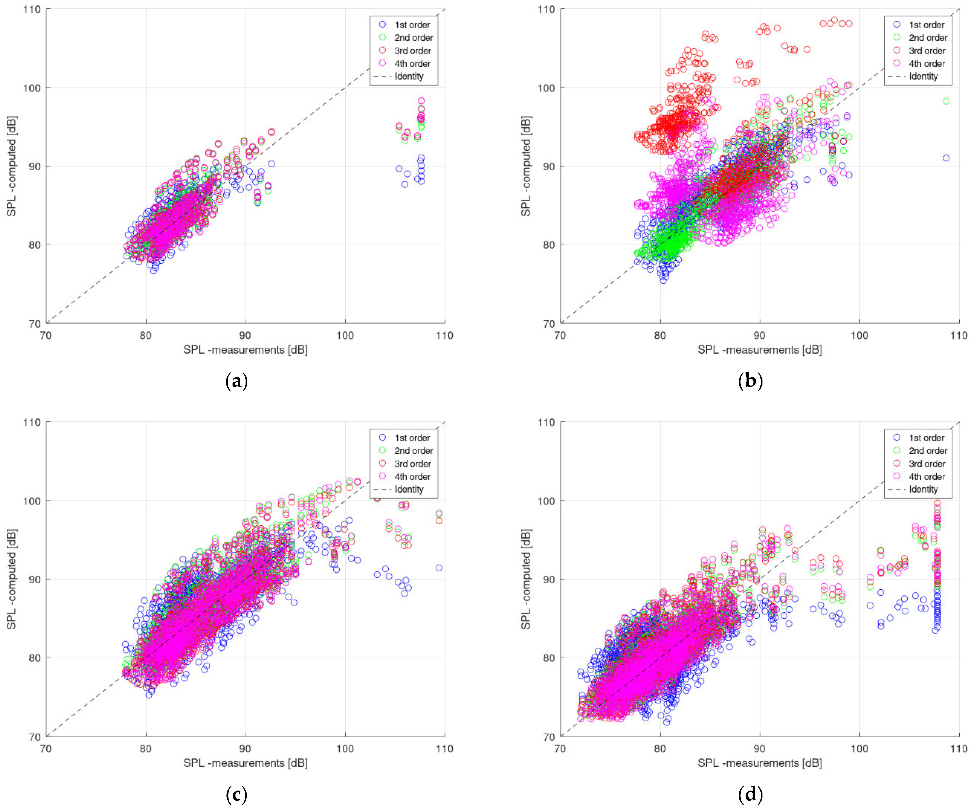
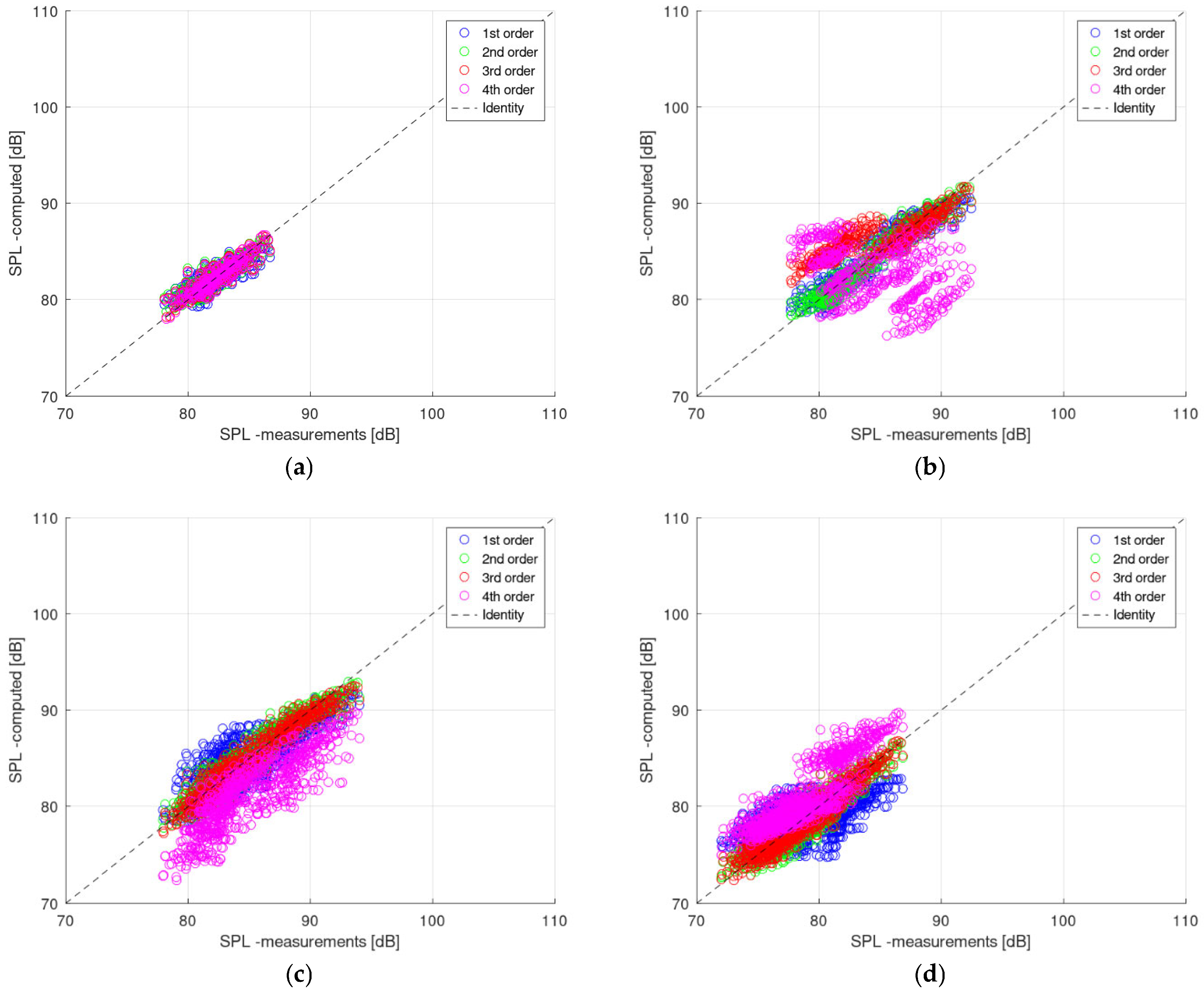
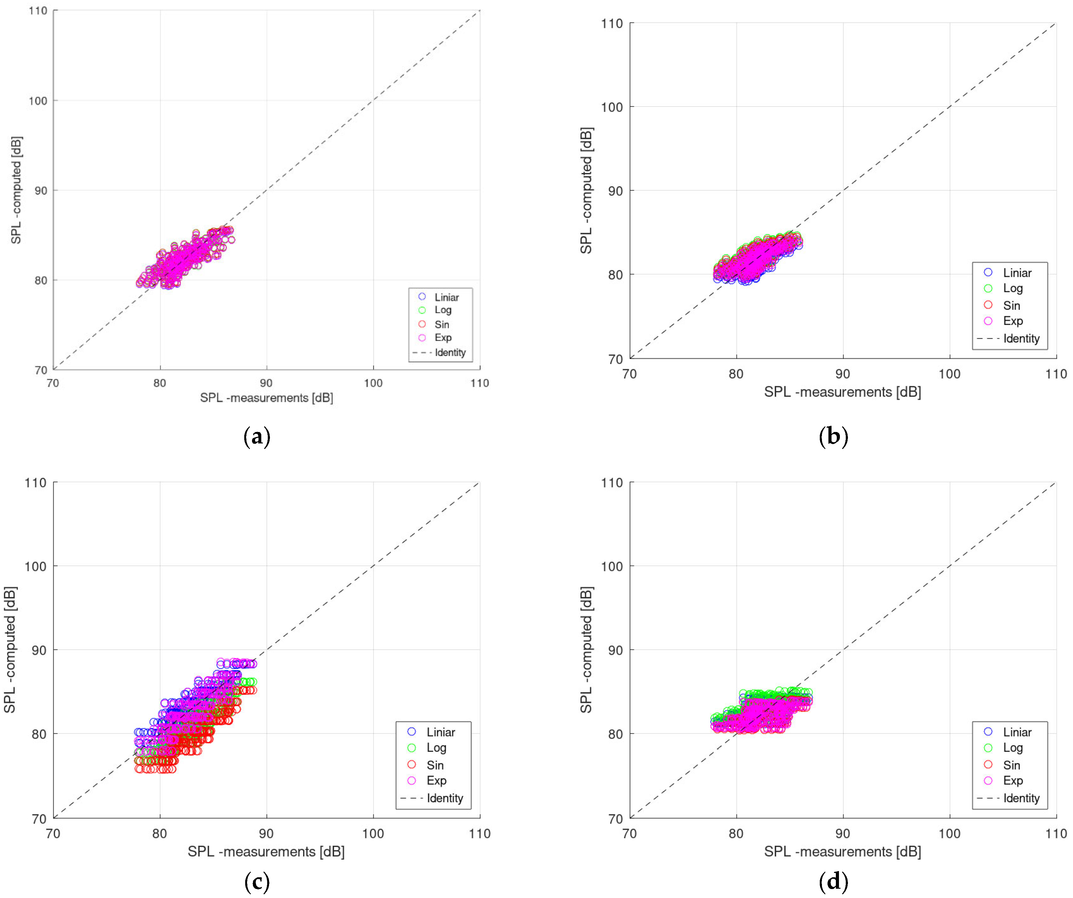
where $y_{ni}$ is normalized SPL, $b_0$ is an intercept term, $b_1-b_{22}$ are coefficients, $x_1=NT/9$, $x_2=\alpha$, $x_3=\theta /\mathrm{m}\mathrm{a}\mathrm{x}\left(\theta \right),$ and $x_4=\phi /\mathrm{m}\mathrm{a}\mathrm{x}\left(\phi \right)$. Theta used in regressions is in the [0, π] range, while phi lies in the [15, 90] degrees range. Alpha is taken as such, with values of 0, 5, 10, or 15 degrees. The aforementioned methods, applied to the existing datasets, led to the overlaps in Figure 3, Figure 4 and Figure 5, with the corresponding R-squared values (and other quantitative indicators) in

Table 1. R² value—all planes data.

	1st Degree	2nd Degree	3rd Degree	4th Degree
α = 0°	0.4151	0.6314	0.6453	0.6469
α = 5°	0.5398	0.7193	−1.9245	0.1198
α = 10°	0.4361	0.6660	0.6666	0.6753
α = 15°	0.3167	0.6387	0.6501	0.6573

,

Table 2. Quantitative indicators; 45–90 deg planes.

	1st Degree			2nd Degree			3rd Degree		4th Degree
	R2	RMSE [dB]	MAE [dB]	R2	RMSE [dB]	MAE [dB]	R2	RMSE [dB]	MAE [dB]	R2	RMSE [dB]	MAE [dB]
α = 0°	0.6683	1.0244	0.83501	0.76502	0.86216	0.65994	0.81812	0.75852	0.57692	0.82398	0.7462	0.55582
α = 5°	0.90965	1.0905	0.88143	0.93967	0.89108	0.72061	0.37118	2.8769	2.3235	−1.2956	5.4968	4.4863
α = 10°	0.68021	2.0171	1.6834	0.92053	1.0055	0.79158	0.91537	1.0376	0.83548	−0.17176	3.8691	3.3737
α = 15°	0.22077	2.5755	2.2534	0.84838	1.1768	0.93275	0.88280	1.0346	0.83153	0.14212	2.7992	2.4108

and

Table 3. R² value for other fitting laws; 45–90 deg planes.

	Linear	Logaritmic	Sin	Exponential
α = 0°	0.6683	0.6750	0.6764	0.6697
α = 5°	0.5238	0.5439	0.5830	0.5849
α = 10°	0.2824	0.1055	−0.1296	0.2878
α = 15°	0.2583	0.1334	0.3064	0.3005

. The specific coefficients of the obtained polynomials are provided explicitly in Appendix A and

Table A1. Regression—full data coefficients (b₀ … b₂₂).

Poly 1st Degree				Poly 2nd Degree				Poly 3rd Degree				Poly 4th Degree
α = 0°	α = 5°	α = 10°	α = 15°	α = 0°	α = 5°	α = 10°	α = 15°	α = 0°	α = 5°	α = 10°	α = 15°	α = 0°	α = 5°	α = 10°	α = 15°
8.5876 × 10−1 −2.7892 × 10−2 4.6998 × 10−18 −4.2708 × 10−2 −7.5972 × 10−2	0.860160 −0.018964 −0.010731 −0.049509 −0.080708	8.5583 × 10−1 −2.7125 × 10−2 −5.0532 × 10−3 −5.0021 × 10−2 −8.1612 × 10−2	8.3935 × 10−1 −2.1251 × 10−2 −1.4749 × 10−3 −4.7614 × 10−2 −8.1235 × 10−2	0.9496 −0.0396 0.0000 −0.2136 −0.2844 0.0171 0.0000 0.0584 0.0948 0.0000 −0.0069 −0.0032 0 0 0.1991	9.5389 × 10−1 −2.8301 × 10−2 2.6040 × 1011 −2.4290 × 10−1 −3.0487 × 10−1 1.0358 × 10−2 −5.2080 × 1010 7.6149 × 10−2 1.0466 × 10−1 3.3569 × 10−3 −9.0188 × 10−3 −6.1837 × 10−3 −2.9269 × 10−3 −2.1433 × 10−3 2.2267 × 10−1	9.6037 × 10-1 −2.0943 × 10−2 −1.4727 × 10−2 −2.4871 × 10−1 −3.1819 × 10−1 1.0778 × 10−2 1.1355 × 10−3 7.5391 × 10−2 1.1008 × 10−1 −1.5555 × 10−3 −1.1993 × 10−2 −5.3604 × 10−3 −8.3378 × 10−4 −7.4498 × 10−4 2.2949 × 10−1	9.6617 × 10−1 −5.1708 × 10−2 −1.3681 × 10−2 −2.4289 × 10−1 −3.1663 × 10−1 3.3104 × 10−2 7.8563 × 10−4 6.7513 × 10−2 1.0871 × 10−1 7.8759 × 10−4 −1.0759 × 10−2 −5.1317 × 10−3 2.4407 × 10−4 −2.0736 × 10−4 2.2573 × 10−1	0.9814 −0.0234 −0.0000 −0.3017 −0.4829 −0.0283 −0.0000 0.2878 0.4892 0.0000 −0.0069 −0.0032 0.0000 0 0.1991 0.0302 0 −0.1529 −0.2254	9.8552 × 10−1 3.9128 × 10−3 −2.4523 × 1012 −3.3699 × 10−1 −4.9849 × 10−1 −5.7400 × 10−2 −1.4099 × 1011 3.2532 × 10−1 4.9461 × 10−1 3.3069 × 10−3 −9.9547 × 10−3 −7.5083 × 10−3 −3.0115 × 10−3 −2.2630 × 10−3 2.2158 × 10−1 4.4461 × 10−2 1.2629 × 1011 −1.6622 × 10−1 −2.2347 × 10−1	9.8556 × 10−1 7.1487 × 10−3 −4.8495 × 1010 −3.1259 × 10−1 −5.2147 × 10−1 −6.4294 × 10−2 1.4548 × 1010 2.4876 × 10−1 5.1925 × 10−1 −1.6219 × 10−3 −1.3166 × 10−2 −6.5164 × 10−3 −9.1351 × 10−4 −8.2349 × 10−4 2.2813 × 10−1 4.9561 × 10−2 −9.6990 × 108 −1.1630 × 10−1 −2.3438 × 10−1	9.9736 × 10−1 −3.2449 × 10−2 −1.9162 × 10−2 −2.8184 × 10−1 −5.2281 × 10−1 −2.0968 × 10−2 1.8353 × 10−3 1.6887 × 10−1 5.1847 × 10−1 7.8759 × 10−4 −1.0759 × 10−2 −5.1317 × 10−3 2.4407 × 10−4 −2.0736 × 10−4 2.2573 × 10−1 3.5974 × 10−2 −4.6652 × 10−5 −6.7570 × 10−2 −2.3415 × 10−1	1.0098 −0.0017 −0.0000 −0.2742 −0.7863 −0.1377 −0.0000 0.1523 1.4686 −0.0000 −0.0069 −0.0032 −0.0000 0.0000 0.1991 0.1988 0 0.0630 −1.4585 −0.0810 0 −0.1080 0.5285	9.6833 × 10−1 −8.2904 × 10−3 −4.3633 × 1012 −2.4343 × 10−1 −7.4005 × 10−1 3.5401 × 10−2 −2.3752 × 1011 −1.0032 × 10−1 1.2864 × 100 3.2452 × 10−3 −1.1535 × 10−2 −8.5843 × 10−3 −3.1544 × 10−3 −2.3603 × 10−3 2.1974 × 10−1 −1.0286 × 10−1 1.7887 × 1011 4.9470 × 10−1 −1.2250 × 100 7.2203 × 10−2 8.6330 × 109 −3.2545 × 10−1 4.3043 × 10−1	1.0078 × 100 −3.1828 × 10−2 −1.0225 × 1011 −1.6299 × 10−1 −7.7702 × 10−1 1.2897 × 10−1 2.6776 × 1010 −4.8840 × 10−1 1.3400 × 100 −1.6003 × 10−3 −1.2906 × 10−2 −6.1013 × 10−3 −8.9606 × 10−4 −7.9550 × 10−4 2.2844 × 10−1 −2.4803 × 10−1 −8.7526 × 108 1.0568 × 100 −1.2660 × 100 1.4299 × 10−1 −7.7982 × 107 −5.8596 × 10−1 4.4162 × 10−1	1.0166 × 100 −1.0273 × 10−1 1.1435 × 1010 −7.8595 × 10−2 −7.7917 × 10−1 3.3121 × 10−1 −4.1930 × 109 −8.2610 × 10−1 1.3424 × 100 8.1032 × 10−4 −1.0691 × 10−2 −4.7493 × 10−3 2.4846 × 10−4 −1.8646 × 10−4 2.2581 × 10−1 −5.0681 × 10−1 4.5742 × 108 1.5129 × 100 −1.2699 × 100 2.6093 × 10−1 −1.5247 × 107 −7.8864 × 10−1 4.4347 × 10−1

and

Table A2. Regression—other laws.

Linear	α = 0°	y = 0.8183 + −0.0288 × x1 + 0.0000 × x2 + −0.0046 × x3 + −0.0482 × x4
	α = 5°	y = 295093271144.8286 + −0.0108 × x1 + −59018654228.8156 × x2 + −0.0064 × x3 + −0.0482 × x4
	α = 10°	y = 67831712699.3154 + −0.0458 × x1 + −6783171269.8535 × x2 + −0.0041 × x3 + −0.0474 × x4
	α = 15°	y = −878484413272.0757 + −0.0044 × x1 + 58565627551.5237 × x2 + 0.0016 × x3 + −0.0479 × x4
Logarithmic	α = 0°	y = 0.8297 + −0.0419 × log(x1 + 1) + 0.0000 × log(x2 + 1) + −0.0053 × log(x3 + 1) + −0.0838 × log(x4 + 1)
	α = 5°	y = 516277507132.0723 + −0.0158 × log(x1+1) + −288139962979.3687 × log(x2 + 1) + −0.0083 × log(x3 + 1) + −0.0838 × log(x4 + 1)
	α = 10°	y = −189824201705.3086 + −0.0658 × log(x1+1) + 79162840787.6846 × log(x2 + 1) + −0.0050 × log(x3 + 1) + −0.0825 × log(x4 + 1)
	α = 15°	y = 3005959750421.1055 + −0.0110 × log(x1 + 1) + −1084170806260.8022 × log(x2 + 1) + 0.0032 × log(x3 + 1) + −0.0835 × log(x4 + 1)
Exponential	α = 0°	y = exp(−0.1985 + −0.0375 × x1 + 0.0000 × x2 + −0.0058 × x3 + −0.0631 × x4)
	α = 5°	y = exp(397079536086.0010 + −0.0152 × x1 + −79415907217.2565 × x2 + −0.0087 × x3 + −0.0680 × x4)
	α = 10°	y = exp(45738065254.1121 + −0.0642 × x1 + −4573806525.4364 × x2 + −0.0056 × x3 + −0.0666 × x4)
	α = 15°	y = exp(−1171057465556.5415 + −0.0058 × x1 + 78070497703.7525 × x2 + 0.0023 × x3 + −0.0651 × x4)
Sinusoidal	α = 0°	y = 0.8276 + −0.0343 × sin(x1) + −0.0000 × sin(x2) + −0.0048 × sin(x3) + −0.0664 × sin(x4)
	α = 5°	y = 379910565179.5400 + −0.0129 × sin(x1) + 396184115072.3145 × sin(x2) + −0.0071 × sin(x3) + −0.0664 × sin(x4)
	α = 10°	y = −249926694732.5410 + −0.0540 × sin(x1) + −459406243123.0117 × sin(x2) + −0.0044 × sin(x3) + −0.0654 × sin(x4)
	α = 15°	y = −737200120072.1660 + −0.0082 × sin(x1) + 1133652014613.7646 × sin(x2) + 0.0022 × sin(x3) + −0.0661 × sin(x4)

.

Other equations for fitting the experimental data have been tried, using as many independent variables, in an attempt to obtain values closer to the experiment. The verified laws are quite general, found in similar works, and they are of the following form:

Logarithmic expression:

$$y_{log}=c_1+c_2·\log \left({\mathrm{x}}_1+1\right)+c_3·\log \left({\mathrm{x}}_2+1\right)+c_4·\log \left({\mathrm{x}}_3+1\right)+c_5·\log \left({\mathrm{x}}_4+1\right)$$

(10)

where, as normalized values are used and mainly in the range [0, 1], a “+1” has been added in the logarithm argument.

Sine or exponential expressions:

$$y_{sin}=c_1+c_2·\sin \left({\mathrm{x}}_1\right)+c_3·\sin \left({\mathrm{x}}_2\right)+c_4·\sin \left({\mathrm{x}}_3\right)+c_5·\sin \left({\mathrm{x}}_4\right)$$

(11)

$$y_{exp}=\mathrm{e}\mathrm{x}\mathrm{p}(c_1+c_2·x_1+c_3·x_2+c_4·x_3+c_5·x_4)$$

(12)

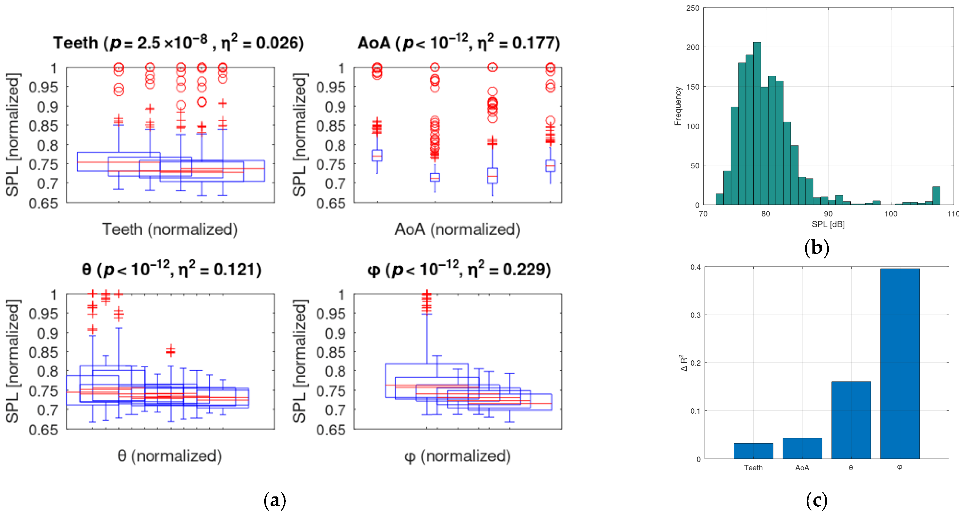
A one-way ANOVA was performed for each of the four independent variables—teeth count, angle of attack (AoA) or blade set angle, polar/lateral angle (θ), and elevation angle (φ)—to assess their statistical influence on the normalized sound pressure level (SPL). The results (Figure 6) indicate that all variables are highly significant, with p-values below 10⁻⁸, confirming that each factor contributes meaningfully to SPL variation. However, the magnitude of each effect varies, as captured by the η² (eta squared) coefficients, which quantify the proportion of total variance attributable to each factor. The elevation angle φ showed the strongest influence (η² = 0.219), suggesting that the position of the observer in the vertical plane has the most pronounced impact on the acoustic measurements. This aligns with the expected sensitivity of jet noise directivity to elevation, especially in cases involving turbulent structures radiating upwards (the directivity of a serrated airfoil-type acoustic source is explicitly formulated in [23] through a function D_h = f(M,θ,ϕ)). The angle of attack α followed with η² = 0.169, indicating that the aerodynamic incidence angle plays a major role in shaping the acoustic response, likely due to modifications in flow interaction with the serrated edge. The polar angle θ contributed a substantial share (η² = 0.113), reflecting the role of azimuthal positioning along the microphone arc in capturing directional lobes of the acoustic field. Lastly, the number of serration teeth had a lower, but still statistically significant effect (η² = 0.026), consistent with previous findings that geometrical changes tend to act as secondary modifiers when compared to flow conditions or observer placement. Together, these results provide quantitative support for the multi-parametric sensitivity of jet noise to both aerodynamic and geometric parameters, and justify the use of multi-dimensional regression models for SPL prediction. The elevation angle φ emerged as the most influential predictor in the ANOVA analysis. This result is physically intuitive, as φ captures the directional dependency of acoustic radiation from the jet–serration interaction zone. Observers at higher elevation angles (closer to the downstream region) are more likely to receive stronger acoustic contributions due to less shielding and a more direct line of sight to turbulent structures. Conversely, lower φ angles (closer to upstream) often result in reduced SPL due to geometric shielding and destructive interference. Therefore, the strong statistical weight assigned to φ is consistent with established aeroacoustic principles governing sound propagation and directivity from complex jet–airfoil interactions.

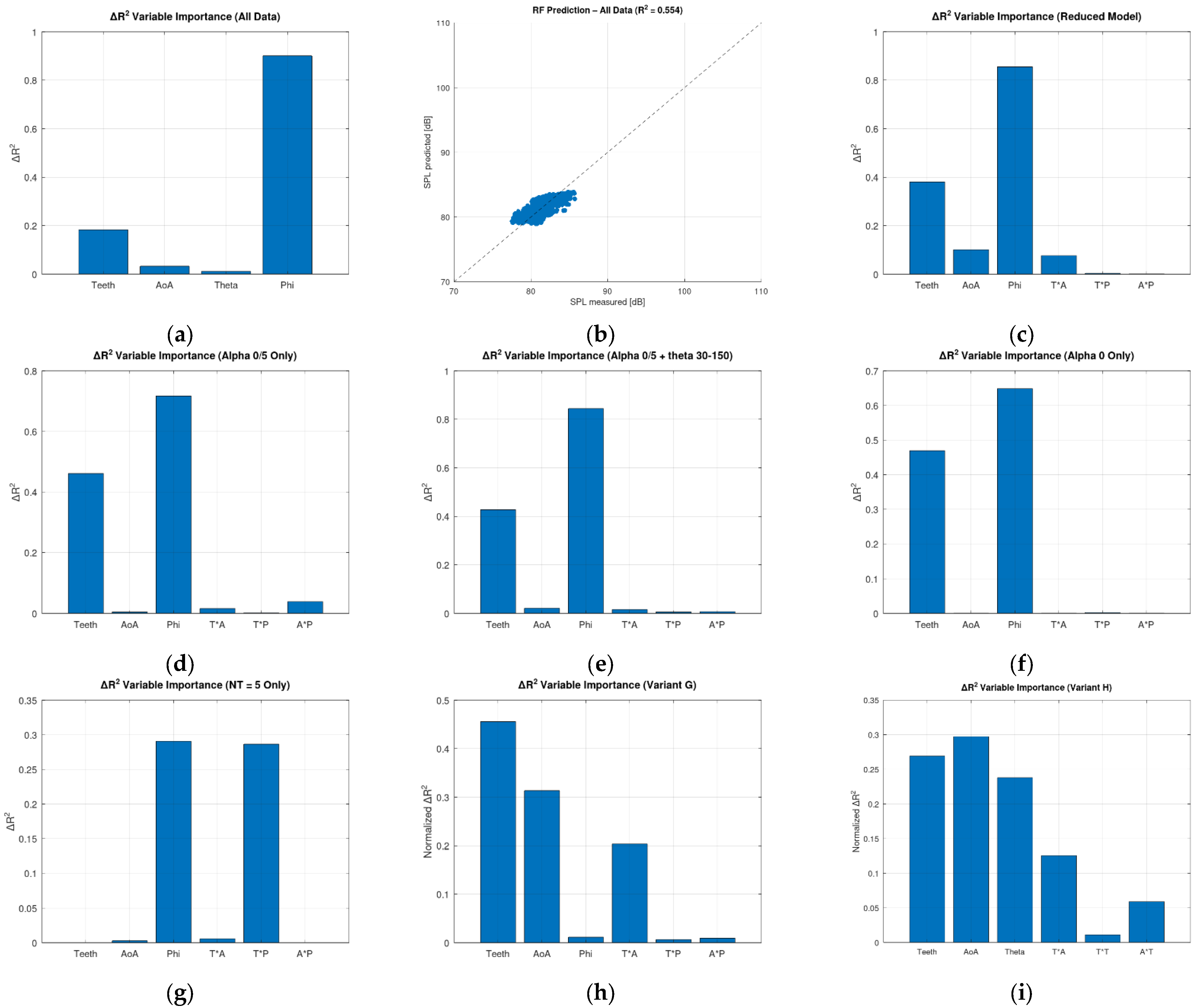
The results of the Random Forest regression applied to each data variant are summarized in

Table 4. Summary of regression results across variants.

Variant	Variables Included/Constraints	No. of Samples	R2	RMSE [dB]	MAE [dB]
A	All variables (NT, α, θ, ϕ)	1040	0.55412	1.007	0.817
B	Reduced variables (NT, α, ϕ) + interactions	1040	0.55417	1.007	0.824
C	α = 0 and 5° only + interactions	520	0.55436	1.046	0.857
D	α = 0 and 5° only, θ = 30–150°	360	0.58876	0.970	0.787
E	α = 0 only, full θ, ϕ, NT)	260	0.54301	1.065	0.867
F	NT = 5 only, all other variables full	208	0.53970	0.904	0.757
G	θ = 90°, ϕ = 45–90°	80	0.69187	0.430	0.355
H	ϕ = 90°only, full θ, all NT, α	260	0.24876	1.177	0.991

. The table includes the variant label, the active variables or constraints applied, the total number of samples used, and the resulting R² value.

The results show that no single regression scenario yielded an R² greater than 0.7, with Variant G providing the best result (R² = 0.692). This variant restricted data to a single observation angle (θ = 90°) and the upper hemisphere (ϕ ≥ 45°), while retaining variability in both installation angle and serration count. This suggests that approximate linear behavior may exist for select configurations but does not generalize well across the full dataset. For other configurations (Variants A–F), R² remained close to 0.55 regardless of the simplifications applied, which confirms that the SPL response is governed by a complex interplay between individual variables and their interactions. This is further supported by the variable importance analyses (ΔR²), which showed that the relative contributions of NT, α, θ, and ϕ vary significantly across subsets (Figure 7). Reducing the dataset to very constrained configurations (e.g., Variant H with ϕ = 90° only) led to a sharp decline in model performance (R² = 0.24876), likely due to insufficient variance or reduced sample counts.

While no configuration achieved excellent predictive performance (R² > 0.9), valuable insights were obtained regarding the sensitivity of SPL to each parameter. The results confirm that multivariate and interaction effects dominate the SPL behavior in serrated LE flows. Future modeling approaches could explore nonlinear methods or augment the dataset to increase predictive robustness.

4. Discussion

The models developed in this study are constrained to the measured configurations, which span serration numbers from 0 to 9, four installation angles (0° to 15°), and acoustic measurements at 13 azimuthal positions (0–180°) across six elevation planes (15° to 90°). Within this domain, extrapolation is feasible along specific axes of variation—particularly for intermediate serration counts and finer increments of angle of attack or observation direction. For global SPL or overall noise metrics, the spherical nature of sound propagation allows for spatial extension of the results beyond the measurement arc, enabling estimation of acoustic output at arbitrary radial positions. Likewise, interpolation across the tested azimuth and elevation directions can be performed with reasonable confidence, provided the acoustic field remains smooth. However, extrapolating outside the measured solid angle—particularly into deep back angles where the nozzle or test rig may act as secondary sources—requires caution, as such regions were not captured experimentally and may include nontrivial reflections or shielding effects.

This study evaluated two distinct regression strategies—functional modeling and ensemble-based regression—for predicting the sound pressure level (SPL) radiated by serrated leading-edge configurations under varied flow and observation conditions. The first approach involved a set of functional regression models, including polynomial expressions (of degrees 1 to 4), as well as logarithmic, exponential, and spline-based fits. These models were applied to normalized input parameters: number of serration teeth (NT), angle of attack (α), and the angular coordinates of observation, namely azimuth (θ) and elevation (φ). A wide range of functional regression models was evaluated in this study to approximate the acoustic radiation (SPL) generated by serrated leading edges under various configurations. Polynomial regression models of degrees 1 through 4 were tested separately for each installation angle (α = 0°, 5°, 10°, 15°), and the results revealed promising accuracy in specific configurations.

The selection of regression methods was closely tied to the characteristics of the experimental dataset. The SPL values, ranging mostly between 80 and 100 dB, exhibited low acquisition noise due to careful test design and measurement stability, thus allowing direct use without aggressive filtering. However, the acoustic responses themselves were inherently nonlinear, influenced by complex interactions between geometrical features (e.g., serration number), installation angle, and observer position. Given this context, polynomial regressions (up to the fourth degree) were initially chosen due to their general-purpose applicability: they are flexible enough to accommodate multiple terms with varied influence and offer interpretable trends without requiring prior assumptions on functional form. Logarithmic and exponential models were tested based on the natural appearance of such relationships in signal processing and sound propagation, where energy decay or amplification often follows similar profiles. Sinusoidal regressions were included, given the oscillatory nature of acoustic waveforms and the periodic variations often observed in directivity patterns. Each of these functional models assumes a specific trend or transformation in the data and is well-suited for capturing dominant tendencies when the physics align with the mathematical structure. In contrast, Random Forest regression was introduced to overcome limitations in functional specificity, offering robustness against unknown nonlinearities and uncovering interactions without requiring an explicit formulation. While no single model type proved universally superior across all cases, the results indicated that higher-order polynomials and Random Forests provided the most accurate fits for constrained subsets of the data, especially when directional and spectral dependencies were strongly expressed.

Polynomial regression was applied up to the fourth degree to approximate SPL variation as a function of normalized geometric and directional parameters. These models assume that the SPL field can be represented by a continuous and smooth polynomial surface. When the data was restricted to higher elevation angles (φ ≥ 45°), second- and third-degree polynomials provided excellent accuracy—e.g., R² = 0.82 for α = 0° and α = 5°—capturing the nonlinear trends in the measured data effectively. However, for the full dataset (including φ = 15° and 30°), performance dropped, and overfitting appeared for higher degrees, with unstable or negative R² values in some cases (e.g., α = 5°, 3rd and 4th degree). This indicates a key limitation: polynomial models are sensitive to dataset size and variability, and their effectiveness depends strongly on restricting the domain to smooth regions of acoustic response.

When limiting the dataset to the more reliable observation planes (i.e., excluding φ = 15° and 30°), the polynomial models achieved high predictive accuracy. For example, second-degree and third-degree polynomial fits yielded R² values above 0.8 for α = 0° and α = 5°, with a peak value of 0.82398 for α = 0° using a fourth-degree fit. These results indicate that the underlying SPL distribution can, in some cases, be effectively captured by parametric models, especially when sufficient data variance and quality are preserved. Conversely, when the full dataset was used—including all φ planes—the polynomial models showed a reduction in performance, with R² scores generally ranging between 0.4 and 0.65. This highlights the sensitivity of regression accuracy to the inclusion of less informative or noisier observation planes. In parallel, alternative functional forms such as linear, logarithmic, sinusoidal, and exponential regressions were tested. These models demonstrated moderate to weak predictive capability, with R² values typically below 0.6. Only in a few instances, such as the sinusoidal model for α = 5°, did the performance exceed 0.58. This further confirms that simpler functional representations—though interpretable—struggle to capture the complex aerodynamic–acoustic relationships across all configurations. Taken together, these findings suggest that functional models can offer robust performance in constrained physical regimes, particularly when both the geometry and observation conditions are carefully selected. However, when the parameter space is broadened, the limitations of low-order regression become more apparent, pointing toward the need for more flexible or data-driven modeling strategies.

Explicit functional regressions using logarithmic, exponential, and sinusoidal terms were tested to reflect known acoustic dependencies (e.g., logarithmic trends with serration spacing or exponential decay with frequency). These methods assume that SPL varies according to a fixed, predefined mathematical form, limiting their flexibility. Although the models provided acceptable results for α = 0° (e.g., R² around 0.67 across all functional forms), their predictive power declined for higher angles, with values dropping below 0.3 or even becoming negative. This underlines a core weakness: these formulations, while theoretically grounded, are insufficient to capture the complex interplay of geometric and directional effects observed experimentally unless further adapted or extended.

To address these limitations, a Random Forest-inspired regression strategy was implemented using custom bootstrap aggregation of linear models in GNU Octave. Rather than relying on built-in machine learning toolkits, the method was constructed explicitly from first principles: each tree in the ensemble was based on a resampled dataset, with regression coefficients estimated via least-squares or pseudoinverse fitting. The ensemble prediction was obtained by averaging over 5000 such regressions. This design preserved transparency and interpretability while emulating the ensemble behavior typical of Random Forests. A total of eight data subsets (Variants A to H) were constructed by selectively constraining the design or observation variables to assess their impact on regression performance. Among these, the best predictive accuracy was obtained in Variant G, which restricted the observation direction to azimuth θ = 90° and elevation ϕ between 45° and 90°, while allowing variation in serration number and installation angle. This configuration yielded an R² value of 0.692, indicating that, under well-constrained physical conditions, linear regression ensembles can approximate SPL with moderate success.

Random Forest-style bootstrapped regression was implemented via ensembles of linear fits over randomized subsets of the data. This approach assumes no global analytical form and instead leverages data-driven variability to approximate SPL. It proved particularly useful when applied to constrained cases such as Variant G (θ = 90°, φ = 45–90°), where it reached R² = 0.69, outperforming most functional models. Its main strength lies in handling interaction effects and nonlinearity without manual tuning, offering robustness even across mixed experimental cases. However, it lacks interpretability: the ensemble does not yield a single governing equation, and performance depends heavily on ensemble diversity and data distribution. Despite these trade-offs, it consistently provided stable and realistic SPL predictions across the test set.

In contrast, when the models were applied to more general cases, such as Variant A (all variables) or Variant B (reduced variables with interactions), the performance remained around R² = 0.55, showing limited predictive power. Moreover, Variant H, which fixed the elevation angle to ϕ = 90°, suffered a sharp drop in accuracy (R² = 0.25), likely due to loss of variability and insufficient statistical representation. These outcomes illustrate the trade-off between physical simplification and data richness: overly constrained configurations may fail to capture general behavior, while overly broad ones may obscure interpretable patterns.

Permutation-based importance analysis (ΔR²) further revealed that the influence of each predictor varies across scenarios. No single parameter emerged as universally dominant; instead, combinations such as NT × α or α × φ were often responsible for the greatest improvements in predictive accuracy, highlighting the coupled nature of geometric and observational influences on SPL generation. Although none of the tested models achieved an R² greater than 0.9, the ensemble regression framework enabled a robust and interpretable approach to modeling serrated leading-edge noise. The findings underline the complexity of aeroacoustic behavior in such configurations and suggest that further improvements may require not only richer datasets, but also hybrid modeling strategies that combine data-driven learning with physically informed constraints.

The practical applicability of the proposed regression-based modeling framework lies in its ability to provide rapid and interpretable estimates of acoustic trends for serrated leading-edge airfoils. By leveraging relatively simple input parameters—such as the number of serrations, installation angle, and observer direction—the models can guide preliminary design decisions aimed at reducing broadband noise emissions. In particular, engineers can use the identified regression relationships to screen multiple geometrical configurations without the need for high-fidelity simulations or extensive wind tunnel testing, thereby accelerating the iterative design cycle. Moreover, the modular structure of the model allows for easy integration into multi-objective optimization pipelines, where acoustic metrics such as SPL or OASPL can be balanced against aerodynamic performance or structural constraints. Since the predictors used in the regression are geometrically and operationally meaningful, the method lends itself well to parametric studies and automated design-space exploration.

Finally, although this study focused on serrated leading-edge configurations, the overall methodology is generalizable and could be extended to other classes of passive noise control geometries, such as trailing-edge serrations, flap-edge treatments, or porous materials. By retraining the regression models on appropriate datasets, the same data-driven strategy could support broader applications in aeroacoustic design and analysis.

5. Conclusions

This study has demonstrated the feasibility and limitations of using both functional and data-driven regression approaches to approximate the acoustic metric (SPL) induced by serrated leading edges under a wide range of geometrical and observational conditions. Polynomial models of second or third degree provided high predictive accuracy for selected installation angles and filtered observation domains, with R² values exceeding 0.8 in the best cases. These models are particularly valuable when interpretability and compact mathematical representation are desired.

However, generalization across all configurations proved challenging. Regression accuracy decreased when using the full experimental dataset or when attempting to model SPL as a function of simplified variable subsets. In such cases, even Random Forest (RF) ensemble models—based on resampled linear fits—struggled to exceed an R² of 0.55. The best RF performance (R² = 0.692) was obtained under restricted observation conditions (θ = 90°, φ ≥ 45°), reinforcing the idea that acoustic directivity and installation parameters jointly shape the SPL patterns in nontrivial ways.

While NT (number of teeth) was used throughout this analysis as a primary geometric input, it is important to note that this parameter can be seamlessly converted into the more conventional form 2 h/λ, where h is the serration amplitude and λ is the tooth spacing. Since the serration amplitude was kept constant across all configurations (peak-to-peak height = 20% of chord), NT intrinsically encodes λ, enabling direct alignment with the established literature and standard scaling laws for serrated edges.

Overall, the results highlight both the potential and the limitations of regression-based acoustic modeling, with strong predictive accuracy achievable under constrained configurations but reduced generalizability across the full parametric space. These outcomes support the notion that future developments should pursue hybrid modeling strategies, combining the interpretability of semi-empirical structures with the flexibility and adaptability of machine learning algorithms. Incorporating richer datasets—featuring increased spatial resolution, expanded spectral content, and possibly full-scale experimental data—could further enhance model reliability and broaden applicability.

Looking forward, several directions are envisioned to increase the practical impact of the approach. First, validating the current models against full-scale experiments or alternative airfoil configurations would help assess robustness and scalability. Second, expanding beyond traditional regression to incorporate more advanced machine learning architectures (e.g., gradient boosting, neural networks) could improve generalization across complex flow scenarios. Lastly, due to its modularity and low computational footprint, the current framework holds promise for integration into multi-objective optimization routines, enabling designers to explore trade-offs between aeroacoustic performance and aerodynamic efficiency, such as minimizing broadband noise while maintaining sufficient lift or structural feasibility.