Decision-Level Multi-Sensor Fusion to Improve Limitations of Single-Camera-Based CNN Classification in Precision Farming: Application in Weed Detection

Abstract

The United States leads in corn production and consumption in the world with an estimated USD 50 billion per year. There is a pressing need for the development of novel and efficient techniques aimed at enhancing the identification and eradication of weeds in a manner that is both environmentally sustainable and economically advantageous. Weed classification for autonomous agricultural robots is a challenging task for a single-camera-based system due to noise, vibration, and occlusion. To address this issue, we present a multi-camera-based system with decision-level sensor fusion to improve the limitations of a single-camera-based system in this paper. This study involves the utilization of a convolutional neural network (CNN) that was pre-trained on the ImageNet dataset. The CNN subsequently underwent re-training using a limited weed dataset to facilitate the classification of three distinct weed species: Xanthium strumarium (Common Cocklebur), Amaranthus retroflexus (Redroot Pigweed), and Ambrosia trifida (Giant Ragweed). These weed species are frequently encountered within corn fields. The test results showed that the re-trained VGG16 with a transfer-learning-based classifier exhibited acceptable accuracy (99% training, 97% validation, 94% testing accuracy) and inference time for weed classification from the video feed was suitable for real-time implementation. But the accuracy of CNN-based classification from video feed from a single camera was found to deteriorate due to noise, vibration, and partial occlusion of weeds. Test results from a single-camera video feed show that weed classification accuracy is not always accurate for the spray system of an agricultural robot (AgBot). To improve the accuracy of the weed classification system and to overcome the shortcomings of single-sensor-based classification from CNN, an improved Dempster–Shafer (DS)-based decision-level multi-sensor fusion algorithm was developed and implemented. The proposed algorithm offers improvement on the CNN-based weed classification when the weed is partially occluded. This algorithm can also detect if a sensor is faulty within an array of sensors and improves the overall classification accuracy by penalizing the evidence from a faulty sensor. Overall, the proposed fusion algorithm showed robust results in challenging scenarios, overcoming the limitations of a single-sensor-based system.

1. Introduction

Precision farming is a technique developed to improve crop yields, reduce chemical usage, and keep environmental impacts at a lower level, and the inclusion of robotics into conventional farming helps in achieving these goals. Researchers have been rigorously studying autonomous weed detection techniques and herbicide application to minimize cost and herbicide usage. There are evidences showing a rise in herbicide resistance among diverse weed species over time [1]. Driven by the need to mitigate labor, cost, and herbicide resistance associated with weed management, there has been significant increase in interest in agricultural robots with autonomous capabilities for weed detection and eradication. The Mechatronics and Autonomous Systems Research Lab (MARL) at Purdue University in Indianapolis has developed one such robot, as shown in Figure 1. This autonomous robot was built by retrofitting a Yamaha Wolverine 4 × 4 All-Terrain Vehicle with a variety of sensors and actuators capable of GPS guided navigation, autonomous weed detection, and herbicide application via a sprayer system [2].

Multi-sensor fusion seeks to overcome the limitations and uncertainties of a single sensor, creates more extensive recognition of the environment around the sensors, and improves the perceptual ability of the system [3]. As an example, a level 4/5 autonomous vehicle can have 4–6 radars, 1–5 Lidars, 6–12 cameras, and 8–16 ultrasonic sensors [4]. Weed classification for autonomous agricultural robots is an equally challenging task for a single-camera-based system due to noise, vibration, and occlusion. To address this issue, we present a multi-camera-based system with decision-level sensor fusion to improve the limitations of a single-camera-based system in this paper.

Researchers have adopted different methodologies to address the challenge of weed detection and classification. Several studies have been conducted [5,6,7] on the classification of UAV-captured images for weed detection. Ahmed et al. [8] proposed an algorithm based on Circular Mean Intensities (CMIs) of weed images to classify weeds into categories like broad weed, narrow weed, and little or no weed. The study did not contain any study on environments where both weeds and crops coexist. Ota et al. [9] proposed a model to detect crops and weeds in a cabbage field using k-means clustering. Chen et al. [10] proposed a multi-feature fusion and support vector machine (SVM) to detect weed and corn seedlings.

The CNN classifier has garnered significant interest in the problem of weed classification in recent years, primarily due to its superior performance in large-scale image classification. For instance, Rodriguez-Garlito et al. [11] used several classification models to detect aquatic invasive plants on the Guadiana River in Spain via images captured through the Sentinel 2-A satellite and found CNN as the best-performing model among K-means classifier, random forest, and CNN. Garibaldi-Marquez et al. [12] studied several SVM and CNN models to classify Zea mays L. (crop), narrow-leaf weeds (NLWs), and broad-leaf weeds (BLWs) and concluded that CNNs were the better models for corn field weed detection, yielding a 97% accuracy. Potena et al. [13] employed two distinct convolutional neural networks (CNNs) to analyze RGB and near-infrared (NIR) images in order to detect crops and weeds. The authors employed a reduced-scale convolutional neural network (CNN) for the purpose of vegetation segmentation, while a more complex CNN architecture was utilized for the categorization of crops and weeds. The classifier produced the highest mean average precision of 98.7%. Sharpe et al. [14] tested a CNN model to detect vegetation indiscriminately and detect and discriminate three classes of vegetation commonly found within Florida vegetable plasticulture row-middles, finding a three-class network outperforming a one-class network with a 95% F score. Reddy et al. [15] compared the performance of the AlexNet architecture with different commonly used architectures like inception-v3, ResNet50, DenseNet, MobileNetV3, etc., for the weedcrop, deepweed, and plantseedlings-v2 databases and observed AlexNet outperforming all of the other models. Espejo-Garcia et al. [16] proposed a crop/weed identification system combining fine-tuning pre-trained convolutional networks like Xception, Inception-Resnet, VGNets, Mobilenet, and Densenet with conventional machine learning classifiers like SVM, XGBoost, and logistic regression. The authors tested the system on two crops (tomato and cotton) and two weed species (black nightshade and velvetleaf) and observed a fine-tuned Densenet and SVM achieving a micro $F_1$ score of 99.29% with minimal performance difference between train and test sets. Sunil et al. [17] compared SVM and VGG16 classification models for four different weed species and six crop species and observed an average $F_1$ score of the VGG16 model classifier between 93% and 97.5%, with a 100% $F_1$ score obtained for the corn class in the VGG16 Weeds–Corn classifier. Yu et al. [18] used the VGGNet architecture to detect weeds in Bermuda grass. They achieved over 95% $F_1$ score and outperformed the GoogleNet architecture. Al-Badri et al. [19] proposed a three-extractor CNN consisting of VGG-16, ResNet-50, and Inception-v3 to classify Rumex Obtusifolius in grasslands and compared it with several different classification methods, obtaining an average of 95.9% $F_1$ score. They conducted a comparative analysis of transfer learning efficacy using six distinct convolutional neural network (CNN) architectures. The objective of their investigation was to evaluate the performance of these designs in the context of sugar beet and volunteer potato detection. The utilization of VGG19 with transfer learning yielded the most notable performance in the context of this binary classification test, achieving an accuracy rate of over 98%. However, according to Suh et al., it has been argued that categorization represents just a single component within the broader process of weed detection. Consequently, the real-time efficacy of an entire pipeline designed for weed detection may be poorer. Olsen et al. [20] conducted training on InceptionV3 and ResNet50 convolutional neural network (CNN) architectures using a dataset of 17,509 tagged pictures encompassing eight distinct weed classes. The researchers attained a level of accuracy over 95%, and the processing time required for their system was deemed suitable for real-time applications. Du et al. [21] compared different popular machine learning frameworks, and based on considerable accuracy and low computational requirements, selected MobileNetV2 to deploy on a Nvidia Jetson Nano-based mobile robot. Nevertheless, convolutional neural networks (CNNs) with multiple layers are more vulnerable to the presence of blurring and noise [22]. Consequently, the accuracy of their classification may decline significantly when attempting to identify weeds from video footage under conditions such as blur, noise, occlusion, vibration, and varying lighting circumstances. The studies discussed above did not explore the limitations derived from the real-time application of deep neural networks, nor did they measure the effects of noise, vibration, or occlusion, or the ways to address them. To ensure the accurate application of herbicides, it is imperative to have a consistent signal from classifiers that can effectively withstand the harsh conditions indicated before. One potential approach to attaining this objective is the utilization of several sensors in conjunction with a sensor fusion framework. This framework facilitates the amalgamation of categorization outcomes obtained from each sensor at the decision-making stage.

The application of conventional chemical weeding involves the uniform spraying of herbicides across the entire field, irrespective of the presence or absence of weeds. This indiscriminate approach leads to significant expenses incurred on herbicides [23] and contributes to severe environmental degradation [24]. However, existing evidence indicates that the growth of weeds occurs in localized regions rather than uniformly throughout agricultural fields. In their study on the occurrence of three distinct grass species in agricultural fields, Marshall et al. [25] demonstrated that a range of 24% to 80% of the sampled area exhibited an absence of grass weeds. Other authors conducted an investigation on a total of seven maize fields and five soybean fields to assess the presence and impact of weeds. According to the survey, around 30% of the cultivated land was found to be devoid of broad-leaf weeds. It was also shown that approximately 70% of the area within the inter-row spacing remained devoid of grass weeds in instances where herbicide application was not implemented. According to Tian et al. [26] and Medlin et al. [27], it was indicated that significant reductions in the quantity of herbicide sprayed may be attained, ranging from 42% (for soybean and maize) to 84% (for maize), based on factors such as weed pressure and number of patches. This implies that by accurately categorizing different types of weeds through continuous video monitoring, farmers or autonomous systems can effectively modify the application rate of herbicides. This endeavor will result in a substantial reduction in the prevalence of herbicide-resistant weeds and a notable decrease in associated treatment expenses.

The utilization of sensor fusion in the field of agricultural robots is significantly constrained. Both LIDAR sensors and vision systems have been employed either independently or in a fused manner to facilitate crop row tracking in sugar beet [28] and rice rows [29]. Studies using LIDAR and a color camera device for detecting tree trunks [30] and autonomous tractor guidance in some crops [31] have been previously published. Farooq et al. [32] proposed a two-camera-based partial transfer learning (CNN) model for weed classification with a 77.4% $F_1$ score. The objective of these endeavors is to establish a system capable of accurately monitoring crop rows across various areas and under varying working conditions. A recent study at Iowa State University [33] employed depth and 2D color data obtained from Microsoft Kinect v2 to detect Lettuce and Broccoli. The Adaboost-based classification model demonstrated superior performance compared to a five-layer neural network, with the lowest test error of approximately 6% for Iowa State. Nevertheless, the utilization of this approach in outside real-time scenarios may require adjustments since Kinect v2 is primarily designed for indoor use. Moreover, the classification task at hand involves a straightforward binary categorization into two classes, namely, crop and non-crop.

Table 1. Summary of weed detection and classification studies.

Study	Sensor/Method	Approach/Architecture	Crop/Weed Type	Performance Metrics
Ahmed et al. (2022) [8]	Image-based	Circular Mean Intensity (CMI)	Broad-Leaf, Narrow-Leaf, No Weed	Classification accuracy: 96%
Ota et al. (2022) [9]	RGB camera	K-means Clustering	Cabbage + Weeds	$F_2$ score for crop detection: 0.919; $F_{0.5}$ score for weed detection: 0.999
Chen et al. (2020) [10]	RGB camera	SVM + Multi-feature fusion	Corn + Weeds	Detection accuracy: 97.5%
Rodriguez-Garlito et al. (2022) [11]	Satellite (Sentinel-2A)	CNN vs. RF vs. K-means	Aquatic Plants	CNN best performance
Garibaldi-Marquez et al. (2022) [12]	RGB	CNN vs. SVM	Zea mays, NLW, BLW	CNN accuracy: 97%
Potena et al. (2016) [13]	RGB + NIR images	Dual CNNs (segmentation + classification)	Crops and Weeds	mAP: 98.7%
Sharpe et al. (2020) [14]	RGB camera	CNN	3 Vegetation Classes	F1 score: 95%
Reddy et al. (2022) [15]	RGB camera	AlexNet, ResNet, DenseNet	Weedcrop, Deepweed, Plantseedlings	AlexNet performed best
Espejo-Garcia et al. (2020) [16]	RGB camera	Fine-tuned CNN + SVM/XGBoost	Tomato, Cotton, Nightshade, Velvetleaf	F1 score: 99.29%
Sunil et al. (2022) [17]	RGB camera	VGG16 vs. SVM	Corn + 10 Total Classes	F1 score: 93–97.5%, Corn: 100%
Yu et al. (2019) [18]	RGB camera	VGGNet vs. GoogLeNet	Weeds in Bermuda Grass	F1 score > 95%
Al-Badri et al. (2022) [19]	RGB camera	VGG-16, ResNet50, Inception-v3	Rumex Obtusifolius in Grassland	F1 score: 95.9%
Olsen et al. (2019) [20]	RGB camera	InceptionV3, ResNet50	8 Weed Classes	Accuracy > 95%
Du et al. (2021) [21]	RGB camera	MobileNetV2 on Jetson Nano	General Weeds	High accuracy, low latency
Dodge et al. (2016) [22]	RGB camera with simulated noise	CNN noise robustness study	General	Accuracy decline under blur/noise
Farooq et al. (2021) [32]	Dual-camera	Partial transfer learning (CNN)	Weed classes	F1 score: 77.4%
Gai et al. (2016) [33]	Kinect v2 (depth + RGB)	Adaboost vs. Neural Net	Lettuce, Broccoli	Test error ∼6% (Adaboost)

provides a comparative analysis of the studies conducted in this field as a summary.

This paper introduces a technique that tackles challenges commonly encountered in single-sensor systems such as noise, vibration, and partial occlusion, and implements a sensor fusion algorithm that addresses scenarios like faulty inputs from a sensor or partial occlusion in multi-sensor systems. The proposed approach involves the implementation of a robust CNN model with a real-time, multi-camera-based sensor fusion algorithm. Firstly, we demonstrate the efficacy of a transfer-learning-based CNN in developing a real-time weed classification system. Secondly, we evaluate the performance of the CNN model using a single camera providing real-time video feed, while discussing the inherent limitations of a single-sensor setup. Finally, we introduce a decision-level sensor fusion algorithm, capable of integrating information from multiple sensors to overcome the limitations of a single-camera system. This research contributes to the field of agricultural technology by providing valuable insights into the advantages and challenges associated with employing sensor fusion techniques in real-time applications.

2. Materials and Methods

2.1. CNN and Transfer-Learning

CNN is a classification model that relies on deep neural networks. This approach constructs image features at various levels of abstraction across multiple layers inside the network. In each layer, a set of kernels (also known as filters) is employed to identify particular forms or objects inside the image representation from the preceding layer. These kernels are structured as matrices with dimensions of either $3\times 3$ or $5\times 5$. The process involves sliding the kernels over the 3D input feature map. The sliding process involves the extraction of a feature that represents a 3D local patch of an image. This is achieved by performing element-wise multiplication of the image data with kernel matrices, which is essentially a convolution operation. Subsequently, the resulting values are summed together [34]. The utilization of layers of convolution allows the model to acquire knowledge about local visual characteristics in a progressively more abstract manner.

In a supervised classification framework, a convolutional neural network (CNN) is composed of a convolutional base, comprising many convolutional layers, followed by fully connected layers at the final stage. The convolutional base generates a feature representation vector for the image, while the fully connected layer transforms this vector into a corresponding class label. The convolution characteristic of convolutional neural networks (CNNs) imparts two noteworthy properties that distinguish them from conventional neural networks [35]:

• CNNs have the ability to acquire translation-invariant characteristics. This implies that when a Convolutional Neural Network (CNN) acquires knowledge about a certain feature located in the upper right corner of one picture, it possesses the capability to identify the same feature in the lower left corner of a different image.
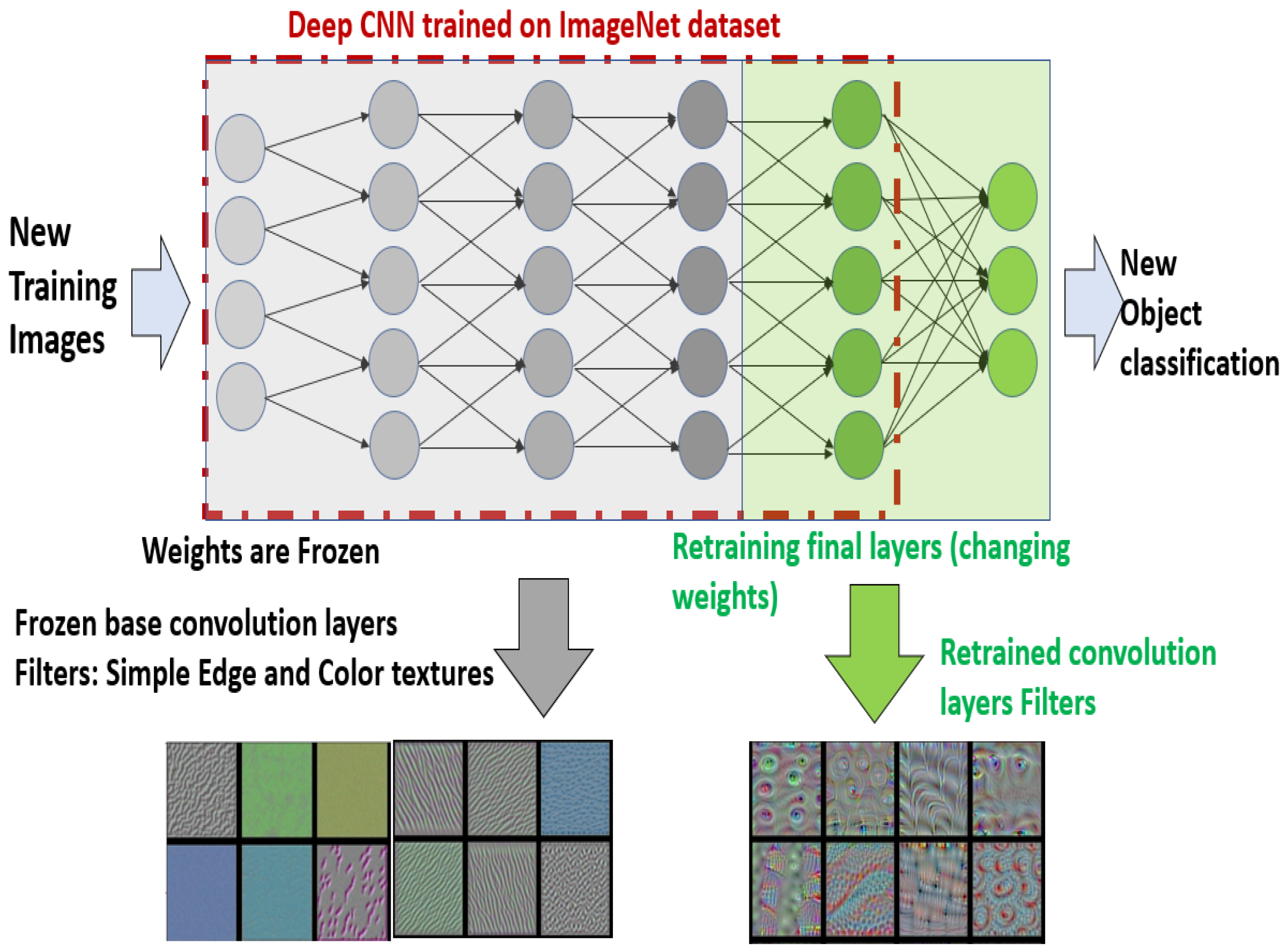
• CNN is capable of acquiring knowledge pertaining to spatial hierarchies of patterns. The initial convolution layers are responsible for acquiring basic visual features such as edges and colors. The second convolutional layer will acquire knowledge of patterns that are composed of patterns from the first layer, such as edges and colors. These patterns may include colored edges and other similar features. The upper layers will acquire a greater understanding of intricate aspects. When the training images pertain to cats, the upper layers of the network will acquire knowledge of distinctive features such as eyes and ears. The aforementioned attribute of CNN allows for the effective utilization of transfer learning, a topic that will be further explored in the subsequent discussion.

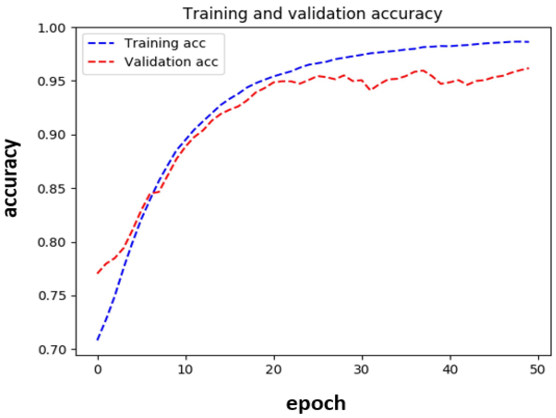
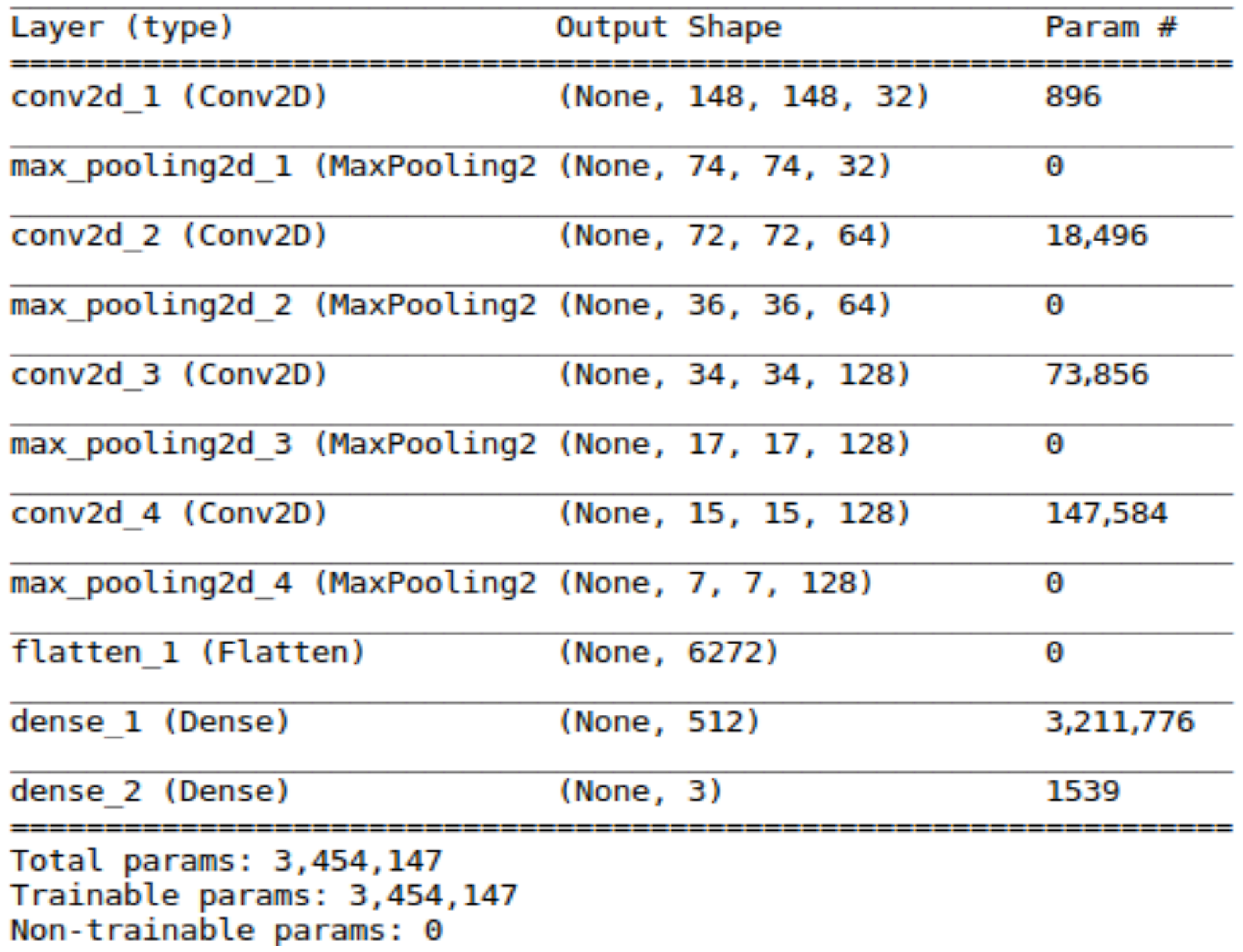
In the context of convolutional neural networks (CNNs), transfer learning refers to the process of utilizing the pre-trained convolutional base of an existing network. This involves employing new training data to retrain the last layers of the CNN, resulting in the creation of a novel classifier that is built upon the existing network. The primary rationale behind employing transfer learning in convolutional neural networks (CNNs) stems from the observation that the initial layers of the network acquire fundamental patterns such as edges and colors, which are commonly present across a wide range of images. Consequently, it is possible to immobilize the weights of these layers and construct a new classifier by solely retraining the latter layers of the CNN. This approach allows the CNN to acquire more advanced features from the input images by leveraging the pre-trained rudimentary features obtained from the early (base) layers. Transfer learning has numerous advantages. One notable benefit is the significant reduction in computation time achieved by leveraging a pre-trained network. This network possesses well-optimized weights in its early layers, resulting in enhanced efficiency. Consequently, favorable training performance can be achieved. Crucially for our objective, achieving satisfactory performance requires only a limited number of training occurrences.

A comprehensive analysis of convolutional neural networks (CNNs) and transfer learning can be found in F. Chollet [35]. Figure 2 shows a simple representation of the architecture of transfer learning.

2.1.1. CNN Model

In this study, we considered a VGG16 [36]-based model architecture with transfer learning. This model is re-trained using a small weed dataset and the final layers are rearranged to classify three different weeds. Transfer learning re-trains the final layers of the VGG16 model to classify new objects from a new dataset by using the large number of features already learned from the Imagenet database. Prior studies [37,38,39] have demonstrated that transfer learning offers significant computational advantages over learning from scratch, and its applicability extends to diverse categorization tasks. The training simulations are executed on a workstation equipped with an Intel Core i7 processor, 8 GB of RAM, and an Nvidia GTX 1060 graphics card with 6 GB of dedicated memory. The construction of models is facilitated through the utilization of the Keras library, which operates on the TensorFlow backend and is implemented in Python 3.5.

2.1.2. Transfer Learning with VGG16

The VGG16 model, which was developed by the Visual Geometry Group, is a convolutional neural network (CNN) that introduced the usage of many small kernel filters as opposed to single-large-kernel filters in its 16-layer design. The VGG16 model was trained using the ImageNet Large Visual Recognition Challenge (ILSVRC) dataset from 2012. During this challenge, the model’s objective was to accurately classify images into 1 of the 1000 available classes. The VGG16 model achieved a top-5 error rate of 7.4% [36].

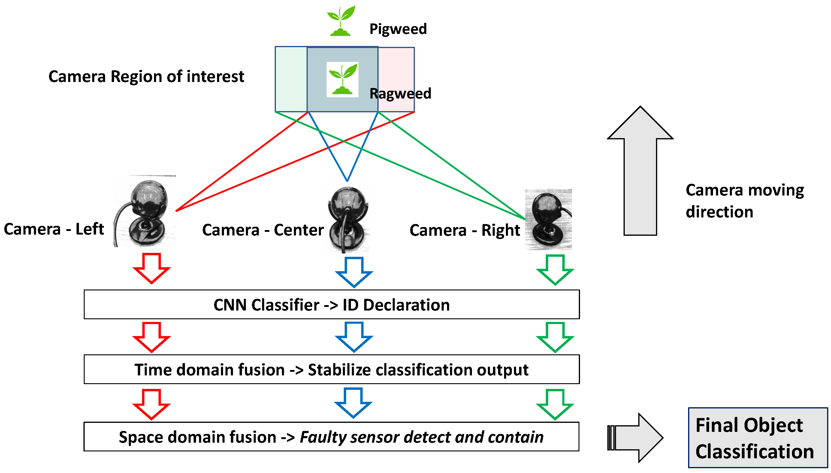
2.2. Decision Level Sensor Fusion

Multi-sensor fusion means the combination of information from multiple sensors (homogeneous or heterogeneous) in a meaningful way that can overcome any limitations inherent to a single sensor or information source [40]. A supervised or unsupervised algorithm (in this study CNN is used) is used to make decisions from available data. Subsequently, the decisions obtained from many sensors are integrated through the utilization of an information fusion method, as depicted in Figure 3. A central challenge at the decision-making stage in multi-source information fusion lies in appropriately representing and resolving imprecise, fuzzy, ambiguous, inconsistent, and potentially incomplete information [41]. Dempster–Shafer (DS) evidence theory, as an uncertainty reasoning method, was proposed by Dempster [42] and further developed by Shafer [43]. The DS evidence theory is a well-established system for managing uncertainty, serving as a means of controlling uncertain environments [44,45]. This evidence theory is extensively utilized in different fields of information fusion, such as decision making [46], pattern recognition [47], risk analysis [48], fault diagnosis [49], and so on [50].

2.2.1. Dempster–Shafer Rule of Combination

The DS combination rule finds the agreement between two or more information sources by taking the orthogonal sum of mass functions. It also handles conflicting evidence by applying a normalization process. The DS combination rule for combining two evidences $m_1$ and $m_2$ is defined as follows:

$$m_{12}\left(A\right)={\displaystyle \frac{{\sum }_{B\cap C}\{m_1\left(B\right)·m_2\left(C\right)\}}{1-K}}$$

(1)

when $A\ne \varphi$ and $m\left(\varphi \right)=0$.

$$K=\sum _{B\cap C=\varphi }\{m_1\left(B\right)·m_2\left(C\right)\}$$

(2)

where K is the degree of conflict in two sources of evidence. ($1-K$) is considered as a normalization factor, which is calculated by adding up the products of BPAs of all sets with null intersections.

2.2.2. Sensor Fusion Algorithm to Eliminate Paradoxes

This study adopts an enhanced Dempster–Shafer (DS) theory for sensor fusion. Compared to Bayesian probability theory, DS theory offers several advantages [51]. However, it also presents certain paradoxes that must be addressed for reliable application. Variations in sensor performance, cluster behavior, and environmental interference can lead to conflicting pieces of evidence. In cases of severe conflict, the fusion results derived from the DS combination rule often contradict intuition. Specifically, when the conflict coefficient K approaches one, the denominator in the combination rule nears zero, resulting in unreasonable fusion outcomes. These unintuitive behaviors are referred to as paradoxes of DS theory. As noted in [52], there are primarily three types of such paradoxes.

• Completely Conflicting Paradox: When there are two sensors and one sensor completely contradicts the other sensor’s output. For example, consider $\Theta =A,B,C$ and
  Sensor 1: $m_1\left(A\right)=0.7,m_1\left(B\right)=0.2,m_1\left(C\right)=0.1$
  Sensor 2: $m_2\left(A\right)=0.0,m_2\left(B\right)=0.9,m_2\left(C\right)=0.1$
  and suppose proposition A is true; then the two sensors provide completely conflicting information. The conflict factor, calculated using Equation (2), is $K=1$, indicating total disagreement between the evidences from sensor 1 and sensor 2. Under such conditions, the DS combination rule becomes inapplicable.
• “One Ballot Veto” Paradox: In a multi-sensor system (with more than two sensors), one sensor may provide an output that completely contradicts the readings from all other sensors. The following example illustrates such a scenario for a given frame. Consider $\Theta =A,B,C$ and suppose proposition A is true, and
  Sensor 1: $m_1\left(A\right)=0.7,m_1\left(B\right)=0.2,m_1\left(C\right)=0.1$
  Sensor 2: $m_2\left(A\right)=0.0,m_2\left(B\right)=0.9,m_2\left(C\right)=0.1$
  Sensor 3: $m_3\left(A\right)=0.75,m_3\left(B\right)=0.15,m_3\left(C\right)=0.1$
  Sensor 4: $m_4\left(A\right)=0.8,m_4\left(B\right)=0.1,m_4\left(C\right)=0.1$
  It is evident that sensor 2 is faulty, as its output contradicts those of the other three sensors. Applying the DS combination rule yields $K=0.9,m_{1234}\left(A\right)=0/0.1=0,m_{1234}\left(B\right)=0.097/0.1=0.97,$ and $m_{1234}\left(C\right)=0.003/0.1=0.03$. These fusion results contradict the assumed proposition that A is true. A high value of K indicates significant conflict among the sensors. This counterintuitive outcome is primarily due to the erroneous readings from sensor 2.
• “Total Trust” Paradox: In this case, one sensor strongly contradicts the other, although they share a common focal element with low supporting evidence. For example, consider the frame $\Theta =A,B,C$ and
  Sensor 1: $m_1\left(A\right)=0.95,m_1\left(B\right)=0.05,m_1\left(C\right)=0$
  Sensor 2: $m_2\left(A\right)=0.0,m_2\left(B\right)=0.1,m_2\left(C\right)=0.9$
  Applying Equation (1) and (2), $m_{12}\left(A\right)=0,m_{12}\left(B\right)=1,m_{12}\left(C\right)=0,$ and $K=0.99$. In this case, common sense indicates that either $m\left(A\right)$ or $m\left(C\right)$ should be correct, yet the incorrect proposition B is identified as true.

The goal of a decision-level sensor fusion algorithm is to combine results from multiple sources so that they can improve the limitations of a single-sensor-based system. Moreover, the fusion algorithm should be able to detect if there is any faulty sensor present in the system and compensate for it. The algorithm under consideration computes the evidence distance originating from each sensor and subsequently assesses the level of agreement or disagreement between sensors. Subsequently, the system provides incentives to sensors that exhibit consensus following their respective levels of information. Sensors with higher information quality get higher rewards. Sensors that disagree with other sensors are penalized so that their evidence has lower weights on the fused result. The method under consideration demonstrates the ability to effectively integrate disparate and contradictory data from numerous sensors, thereby addressing a notable constraint inherent in the original DS combination rule. Here the description follows the approach taken by [40,53] to describe the relevant algorithm:

• Step 1: Construct a multi-sensor information matrix for space domain fusion by considering a system with N sources of evidence (sensors) within the frame $\Theta =\{H_1,H_2,\dots ,H_M\}$ representing the objects to be classified.

  $$\left(\begin{array}{cccc}{m}_1\left(H_1\right)& m_1\left(H_2\right)& \dots & m_1\left(H_M\right)\\ m_2\left(H_1\right)& m_2\left(H_2\right)& \dots & m_2\left(H_M\right)\\ ⋮& ⋮& \ddots & ⋮\\ m_N\left(H_1\right)& m_N\left(H_2\right)& \dots & m_N\left(H_M\right)\end{array}\right)$$

  (3)

For time domain fusion, assume there are N time-steps in the frame $\Theta =\{H_1,H_2,\dots ,H_M\}$.

$$\left(\begin{array}{cccc}{m}_1\left(H_1\right)& m_1\left(H_2\right)& \dots & m_1\left(H_M\right)\\ m_2\left(H_1\right)& m_2\left(H_2\right)& \dots & m_2\left(H_M\right)\\ ⋮& ⋮& \ddots & ⋮\\ m_N\left(H_1\right)& m_N\left(H_2\right)& \dots & m_N\left(H_M\right)\end{array}\right)=\left(\begin{array}{c}{t}_1\\ t_2\\ ⋮\\ t_s\end{array}\right)$$

(4)

• Step 2: Measure the relative distance between the evidence. Consider two mass functions $m_i$ and $m_j$ defined over the discriminant frame $\Theta$; the Jousselme distance between $m_i$ and $m_j$ is defined as follows:

  $$DM(m_i,m_j)=\sqrt{{\displaystyle \frac{1}{2}}.(m_i-m_j)·D·{(m_i-m_j)}^T}$$

  (5)

  where $D={\displaystyle \frac{|A\cap B|}{|A\cup B|}}$ and |.| indicates cardinality.
• Step 3: Compute the total evidence distance for each sensor.

  $$d_i=\sum _{j=1\&j\ne i}^{N}DM(m_i,m_j)$$

  (6)
• Step 4: Compute the global average of evidence distance.

  $$\overline{d}={\displaystyle \frac{{\sum }_{i=1}^N{d}_i}{N}}$$

  (7)
• Step 5: Determine the belief entropy of each sensor based on Equation (9) and perform normalization.
• Step 6: The set of evidence is divided into two categories: credible evidence and incredible evidence, as defined by Equations (13) and (14):

  $$\begin{array}{c}\hfill If{d}_i\le \overline{d},m_{i}iscredibleevidence\\ \hfill If{d}_i>\overline{d},m_{i}isincredibleevidence\end{array}$$

  (8)

The credible evidence is rewarded so that it has more weight in the final fused result. The incredible evidence is detected as a faulty sensor and penalized. The following reward and penalty functions are used:

$$\begin{array}{c}\hfill Credibleevidence,Reward:=-ln\left(\overline{E_P\left(m\right)}\right)\\ \hfill Incredibleevidence,Penalty=-ln(1-\overline{E_P\left(m\right)})\end{array}$$

(9)

Perform normalization on reward and penalty values to derive evidence weights.

• Step 7: Update the original evidences.

  $$m\left(A\right)=\sum _{i=1}^N{m}_i\left(A\right)·w_i$$

  (10)

  where $w_i$ is the sensor evidence weight.
• Step 8: Aggregate the modified evidence for ($n-1$) times (n is the number of sensors) with the DS combination rule by using Equations (1) and (2).

The proposed decision-level sensor fusion algorithm has multiple advantages:

• Enhances the constraints of the first DS combination principle.
• Combines results from both homogeneous and heterogeneous sensors at the decision level.
• Has the capability to identify and rectify malfunctioning sensors, thus ensuring that the inaccurate readings from these sensors do not adversely impact the fused findings.

Algorithms 1 and 2 present the pseudocode for the two processes. The reduced format of this method, together with the final output, is illustrated in Figure 4. Initially, a three-dimensional information matrix is generated to encompass all the sensor evidence collected over the time interval from $t_1$ to $t_s$. In the context of time domain fusion, the fusion process involves integrating information from all the chosen time steps, resulting in the production of a two-dimensional matrix as the output. In the context of space domain fusion, the fusion process involves integrating input from several sensors. The resulting output is a vector that encompasses categorization evidence, represented as a percentage output, for each individual item.

Algorithm 1 Time Domain Fusion using Multiple Sensors

1: Input: Sensor data from left, center, and right cameras   2: Output: Fused classification percentages for Pigweed and Ragweed   3: Load sensor data   4: Extract Pigweed and Ragweed data from each sensor   5: Define information matrices for each camera   6: Set parameters: time steps (ts) and number of objects   7: for each time window do   8:    for each time step in the window do   9:    Compute distance matrix D 10:    Compute entropy 11:    Calculate normalized entropy and rewards 12:    Determine weights and initial evidence 13:    Perform evidence fusion 14:    Store fused evidence 15:   end for 16: end for 17: Extract and plot original and fused classification percentages 18: Plot: Original and fused classification percentages

Algorithm 2 Space Domain Fusion using Multiple Sensors

1: Input: Information matrix M from multiple sensors   2: Output: Fused evidence for classification   3: Step 1: Define information matrix M   4: Step 2: Compute distance matrix D   5: for each sensor pair do   6:    Calculate Jousselme distance $D_{ij}$ for sensor pairs   7: end for   8: Construct distance matrix $DM$   9: Step 3: Calculate average evidence distance d 10: Step 4: Compute entropy for each sensor 11: Normalize entropy values 12: Step 5: Calculate rewards and penalties 13: Normalize evidence weights 14: Step 6: Modify original evidence using weights 15: Step 7: Perform evidence fusion iteratively 16: for each sensor combination do 17:    Calculate fusion matrix 18:    Compute combined evidence 19: end for 20: Output: Fused evidence for classification

2.3. Methodologies

The proposed system is developed following a three-step methodology. Initially, a weed image dataset is curated, and the CNN model is trained using this dataset. Subsequently, the trained model is evaluated in a test environment utilizing a single-camera-based video feed in different scenarios. Finally, a multi-sensor-based sensor fusion algorithm is implemented to overcome limitations observed in the single-camera feed and also address common issues such as the presence of a faulty sensor and partial occlusion. The output from the weed classification process is integrated into the control spray mechanism of the AgBot used in the test environment. The classification and spray system pipeline is demonstrated in Figure 5.

2.3.1. Weed Image Dataset and Image Processing

A widely accessible 16-megapixel digital camera was used to capture photos to construct the dataset. The IUPUI Greenhouse cultivated three common species of corn weeds: Xanthium strumarium (Common Cocklebur), Amaranthus retroflexus (Redroot Pigweed), and Ambrosia trifida (Giant Ragweed) for this purpose. Additionally, we visited real corn fields during the summer to photograph weeds. Sample photographs are shown in Figure 6. The study used a maximum input image size of 150 by 150 pixels, corresponding to the input dimension of the convolutional neural network (CNN), which the 16-megapixel camera supported adequately. The dataset comprises 1993 images in total, with the distribution across different classes and sets presented in

Table 2. Weed image dataset.

Dataset	Cocklebur	Pigweed	Ragweed	Total
Train image set (used for training the classifiers)	544	505	552	1601
Validation image set (used for tuning hyperparameters)	65	62	69	196
Test image set (used for classification report)	65	62	69	196
Total images	674	629	690	1993

. Given that transfer learning has proven effective for small datasets [54] and is widely used in medical applications [55,56], and since there were no suitable open-source datasets available for our specific needs, we were motivated to create our own dataset. In this study, we observed that a dataset of nearly 2000 images was sufficient to achieve satisfactory results. No augmentation techniques were employed to enhance the dataset size.

2.3.2. Conducting Transfer Learning on VGG16

The next step involved conducting transfer learning on a pre-trained VGG16 model. This VGG16 model was originally trained using a subset of the ImageNet dataset for ILSVRC 2012, which contains 10 million images representing over 1000 object types. We re-trained this model with our weed image dataset. The entire dataset was split into three distinct mutually exclusive subsets, training, validation, and test datasets, with an approximate split of 80%, 10%, and 10%, respectively, to maintain the essential principle of supervised learning. The training set was used to train the CNN classifiers with image instances, while the validation set helped optimize the model’s hyperparameters. Finally, the test set was reserved for evaluating and reporting the model’s performance. The class-wise image counts are detailed in Table 2. For training this model, a learning rate of 1 × 10⁻⁵, the Adam optimizer, and the sparse categorical cross-entropy loss function were used. The model, pre-trained on ImageNet subsets, underwent transfer learning for 50 epochs.

2.3.3. Real-Time Classification from Single-Camera Video Input

The experimental environment was designed to evaluate the algorithm under controlled conditions since it was challenging to find weed collocations in the field. To evaluate the performance of the CNN classifier using a single-camera video feed, we designed four specific scenarios. These scenarios were devised to assess the accuracy and stability of the classifier’s output. In the first scenario, a potted Pigweed plant was placed, and the camera was moved over the plant to simulate the movement of an AgBot camera across a weed patch. In the second scenario, a Ragweed plant and a Pigweed plant were positioned in such a way that the camera view did not overlap the two different plant types during the video recording. The third scenario involved introducing artificial Gaussian and salt-and-pepper noise into the images, which were then subjected to classification by the CNN classifier. Lastly, in the fourth scenario, three stages of linear blurriness (low: 10%, medium: 25%, high: 40%) were artificially applied to the weed images before being evaluated by the classifier. The videos were captured using a 12-megapixel digital camera placed approximately 2 feet above the plant at a 45-degree angle.

2.3.4. Implementation of Sensor Fusion Algorithm

To address the possible issues associated with single-camera video feeds, an array of three cameras placed side-by-side with each other at a constant distance was used. All three cameras focused on the same subject that was present directly in front of the center camera. This test scenario was developed to address the shortcomings associated with a single-sensor classification system. Two different operating conditions were simulated. In the first scenario, one sensor provides faulty output, and in the second case, two out of three cameras are partially occluded. Classification accuracy with the CNN classifier is monitored for both conditions and finally, space and time domain sensor fusion is applied in both cases to observe an improvement in outputs.

3. Results

3.1. Classification Report

Figure 7 shows the training and validation accuracy of the trained CNN model. The training accuracy smoothly improves and reaches 99% after 50 epochs. The validation accuracy also reaches over 95% and simulation is stopped. One interesting aspect is that both training and validation accuracy start at over 70% accuracy at epoch zero. This is one of the biggest advantages of transfer learning over training from scratch. Because we already started with a pre-trained model on Imagenet, it was able to achieve that accuracy at the beginning, saving a lot of simulation time and reducing the possibility of overfitting.

Table 3. Confusion matrix based on test image set.

True Label	Cocklebur	65	0	0
	Ragweed	4	55	3
	Pigweed	0	4	65
		Cocklebur	Ragweed	Pigweed
	Predicted label

shows the confusion matrix of the model. From the confusion matrix, it is clear that Ragweed is the hardest one to classify. The CNN model misclassified Ragweed as Cocklebur/Pigweed in seven instances.

We trained two additional models with this dataset to present a comparative study of the model’s performance. The first model is a small six-layer CNN, designed as a simplified version of VGG16 to suit the smaller dataset better. Although the structure mirrors that of VGG16, the number of parameters is significantly reduced. Figure 8 illustrates the architecture of this model. For training, we used a learning rate of 1 × 10⁻⁴, the RMSprop optimizer, and sparse categorical cross-entropy loss. The second model is InceptionResNetV2, which was similarly pre-trained on an ImageNet subset and subsequently fine-tuned with our image dataset. The parameters for this model included a learning rate of 2 × 10⁻⁵, the RMSprop optimizer, and sparse categorical cross-entropy loss. This model also underwent transfer learning for 50 epochs. The comparative classification report, including inference times, is shown in

Table 4. Comparative classification report of the three models: 6-layer CNN (model-1), transfer-learned InceptionResNetV2 (model-2), and transfer-learned VGG16 (model-3). C = Cocklebur; R = Ragweed; and P = Pigweed. Inference time (classifying image to infer a result) tested on a Core i5, 8 GB RAM machine.

	Model-1			Model-2			Model-3
	C	P	R	C	P	R	C	P	R
Precision	0.79	0.74	0.89	0.96	0.92	0.79	0.94	0.94	0.96
Recall	1	0.68	0.74	1	0.7	0.94	1	0.89	0.94
F1 score	0.88	0.71	0.81	0.98	0.79	0.86	0.96	0.94	0.95
Training accuracy	0.85			0.97			0.99
Validation accuracy	0.8			0.93			0.97
Testing accuracy	0.81			0.88			0.94
Image size	150 × 150 × 3			299 × 299 × 3			150 × 150 × 3
Inference time	0.064 s (CPU)			3.68 s (CPU)			0.266 s (CPU), 0.032 s (GPU)

. The proposed model demonstrates the highest recall for all weed classes and the highest precision and F1 score for the Pigweed and Ragweed classes. Notably, Pigweed classification poses a significant challenge, as evidenced by the recall rates of the CNN models, with the proposed model achieving the highest recall at 0.89. Inference time is crucial for real-time categorization derived from video inputs. Here, all of the models were trained on a Core i5, 8 GB RAM machine. Although the small six-layer CNN model had the fastest inference time, the proposed model’s inference time of 0.266 s, resulting in approximately four frames per second (FPS) in our test scenario, was satisfactory, especially considering the performance metrics and the lack of GPU acceleration. When utilizing GPU acceleration, specifically with the Nvidia GTX 1060 Ti, the proposed model achieved a performance rate of approximately 30 FPS.

3.2. Real-Time Classification from a Single Camera Video Input

3.2.1. 1 Pigweed in Video Frame (Figure 9)

In a 30 s video input, a full Pigweed plant appears in the frame for 26 s. During this period, the classifier achieves nearly 100% accuracy in identifying Pigweed. After the 26 s mark, the Pigweed plant moves out of the frame, leading to partial occlusion and resulting in occasional misclassifications. Overall, the classifier reliably delivers stable and accurate identification in real-time video when only a single type of weed plant is present.

Figure 9. Classification accuracy from video input using fine-tuned VGG16. Only one Pigweed plant on video.

Figure 9. Classification accuracy from video input using fine-tuned VGG16. Only one Pigweed plant on video.

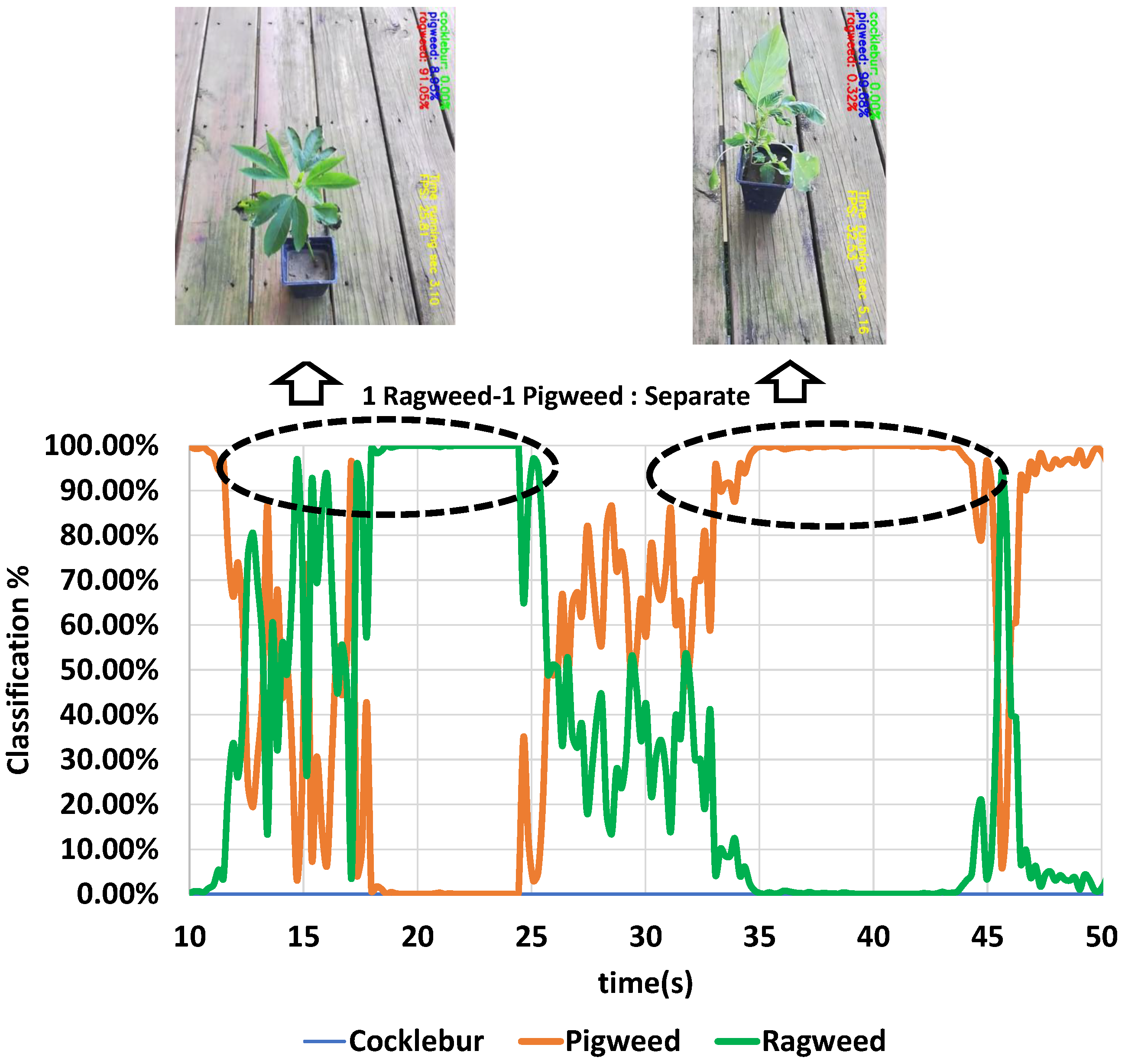
3.2.2. 1 Ragweed and 1 Pigweed in the Video, Separately Placed (Figure 10)

In a 50 s video input, Ragweed is visible in the frame during the first 25 s before gradually moving out, while Pigweed enters the frame. For Ragweed, classification IDs are unstable between 12 and 18 s, with additional instability occurring during the transition period from 25 to 35 s. Despite these fluctuations, the model overall achieves high accuracy in classifying both plants. It effectively manages real-time transitions between different plant types. These two scenarios commonly occur in corn fields.

Figure 10. Classification accuracy from video input using fine-tuned VGG16. One Pigweed plant and one Ragweed plant on video, separately placed.

Figure 10. Classification accuracy from video input using fine-tuned VGG16. One Pigweed plant and one Ragweed plant on video, separately placed.

3.2.3. 1 Ragweed in the Frame, Noise Artificially Introduced (Figure 11)

The robustness of the proposed model was evaluated by introducing artificial noise—specifically Gaussian and salt-and-pepper noise—into the images. Such noise, often caused by field conditions or low-quality sensors, can degrade classifier accuracy. However, as illustrated in Figure 11, the presence of noise in the input images does not significantly impact the classifier’s performance. Additionally, variations in noise intensity up to a certain level were found to have minimal effect on classification accuracy. This resilience is likely due to the deep architecture of the VGG16 network, which enables it to learn features that remain robust in the presence of noise [22]. The initial layers are more susceptible to the influence of high-frequency noise. The impact of noise on the responses of the latter layers is comparatively lower compared to the initial layers. Transfer learning was employed in this study to just retrain the final layers of the VGG16 network. This factor may contribute to the enhanced resilience of the classifier in the presence of noise.

Figure 11. Effect of Gaussian and salt-and-pepper noise on classification accuracy.

Figure 11. Effect of Gaussian and salt-and-pepper noise on classification accuracy.

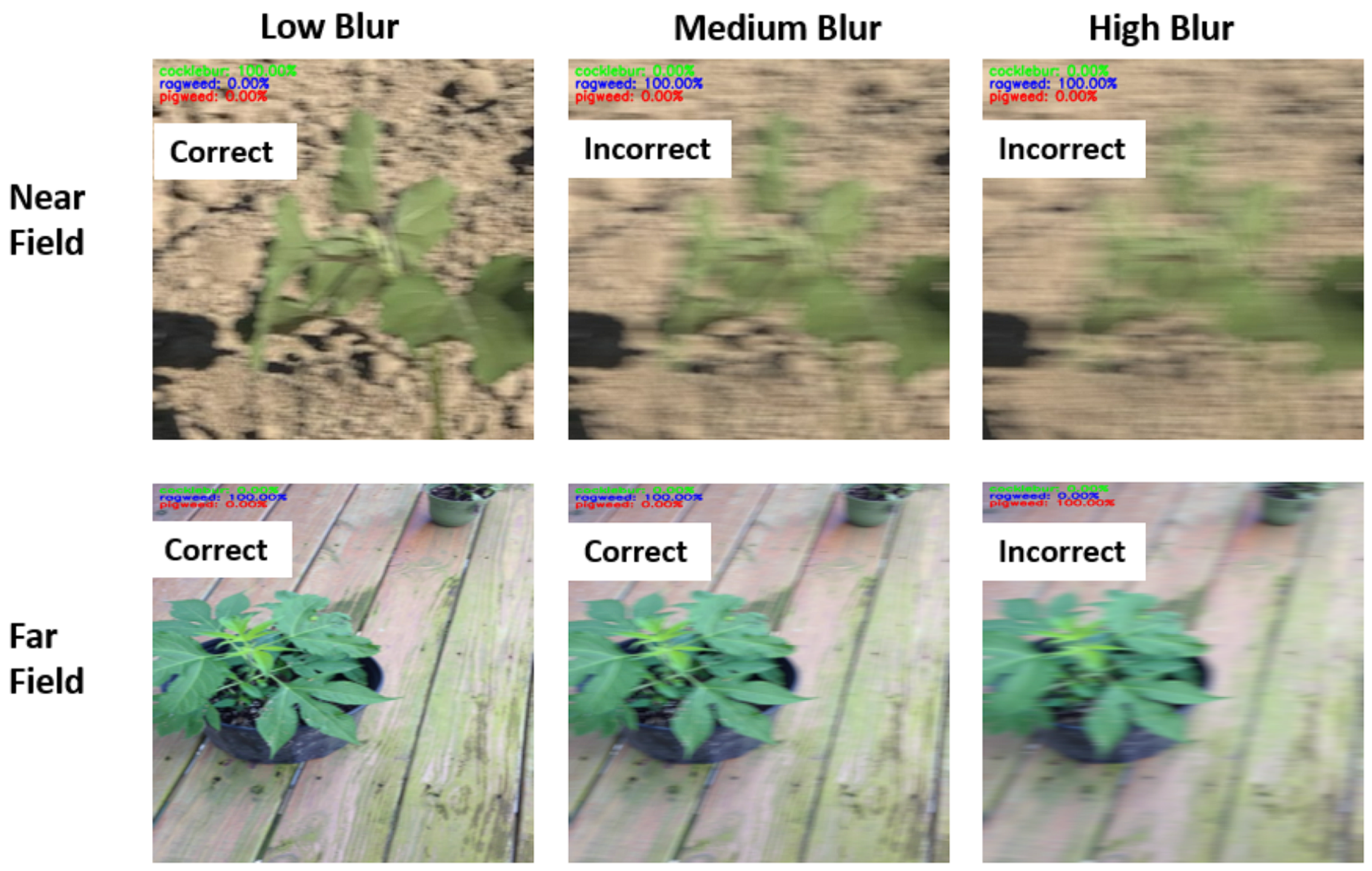
3.2.4. 1 Ragweed in the Frame, Blurriness Artificially Introduced (Figure 12)

The proposed model also shows good results in scenarios where blurriness was introduced to mimic camera vibrations. In the context of low blur, accurate classification is achieved for both nearby and distant field images. Incorrect classification in near-field contexts happens when medium and high levels of blur are present. In the context of far-field analysis, inaccurate categorization is observed exclusively in conditions of significant blurring. The influence of motion blur on the accuracy of image categorization is more pronounced for near-field images than for far-field images. This observation suggests that positioning the camera at a distance that effectively captures the distinguishing characteristics of the weed plants from the greatest feasible distance is advisable. Moreover, conventional masks such as the Unsharp Mask and Gaussian Mask are ineffective in rectifying motion blurriness when it is severe. This observation suggests that the retrieval of lost information resulting from motion blur is a significant challenge.

Figure 12. Effect of different levels of blur on classification accuracy.

Figure 12. Effect of different levels of blur on classification accuracy.

It is evident that while the proposed algorithm can mitigate the impact of noise and vibration on classification accuracy to some extent, it is unable to consistently produce accurate outputs in all situations. However, achieving a stable and accurate weed classification output is crucial for the correct functioning of the herbicide spray system. In both Figure 9 and Figure 10, it is observed that when the weed is partially occluded due to camera movement, the classification becomes unstable, and the output from the CNN classifier is insufficiently clear to trigger a signal for the herbicide spray system. Furthermore, in the event of a sensor failure during operation, the entire system would become inactive. To overcome these limitations and enhance the overall robustness of the system, a decision-level multi-sensor fusion algorithm is proposed in the next section. This algorithm aims to address these challenges and improve the system’s reliability and stability.

3.3. Sensor Fusion-Based Weed Detection Under Different Operating Conditions

3.3.1. Performance Analysis of the Proposed Method

The theoretical foundation and effectiveness of the proposed method are demonstrated in [40], where the following analysis is presented. Consider a multi-sensor system with three target types, $A,B,C$, where A is the true target. The basic probability assignment (BPA) from four sensors is listed below.

• Sensor 1: $m_1\left(A\right)=0.41,m_1\left(B\right)=0.29,m_1\left(C\right)=0.3$
• Sensor 2: $m_2\left(A\right)=0.0,m_2\left(B\right)=0.9,m_2\left(C\right)=0.1$
• Sensor 3: $m_3\left(A\right)=0.58,m_3\left(B\right)=0.07,m_3(A,C)=0.35$
• Sensor 4: $m_4\left(A\right)=0.55,m_4\left(B\right)=0.1,m_4(A,C)=0.35$

Here, sensor 2 provides outputs that contradict those of the other sensors. The comparison of evidence combination with respect to other similar methods is shared in

Table 5. Results of different combination methods for the given example [40].

Methods	${\mathit{m}}_{12}$	${\mathit{m}}_{123}$	${\mathit{m}}_{1234}$
Dempster [42]	m(A) = 0, m(B) = 0.8969, m(C) = 0.1031	m(A) = 0, m(B) = 0.8969, m(C) = 0.1031	m(A) = 0, m(B) = 0.8969, m(C) = 0.1031
Murphy [57]	m(A) = 0.0964, m(B) = 0.8119, m(C) = 0.0917, m(AC) = 0	m(A) = 0.4619, m(B) = 0.4497, m(C) = 0.0794, m(AC) = 0.0090	m(A) = 0.8362, m(B) = 0.1147, m(C) = 0.0410, m(AC) = 0.0081
Deng [58]	m(A) = 0.0964, m(B) = 0.8119, m(C) = 0.0917, m(AC) = 0	m(A) = 0.4974, m(B) = 0.4054, m(C) = 0.0888, m(AC) = 0.0084	m(A) = 0.9089, m(B) = 0.0444, m(C) = 0.0379, m(AC) = 0.0089
Han [59]	m(A) = 0.0964, m(B) = 0.8119, m(C) = 0.0917, m(AC) = 0	m(A) = 0.5188, m(B) = 0.3802, m(C) = 0.0926, m(AC) = 0.0084	m(A) = 0.9246, m(B) = 0.0300, m(C) = 0.0362, m(AC) = 0.0092
Wang [60] recalculated	m(A) = 0.0964, m(B) = 0.8119, m(C) = 0.0917, m(AC) = 0	m(A) = 0.6495, m(B) = 0.2367, m(C) = 0.1065, m(AC) = 0.0079	m(A) = 0.9577, m(B) = 0.0129, m(C) = 0.0200, m(AC) = 0.0094
Jiang [61]	m(A) = 0.0964, m(B) = 0.8119, m(C) = 0.0917, m(AC) = 0	m(A) = 0.7614, m(B) = 0.1295, m(C) = 0.0961, m(AC) = 0.0130	m(A) = 0.9379, m(B) = 0.0173, m(C) = 0.0361, m(AC) = 0.0087
Proposed	m(A) = 0.0057, m(B) = 0.9691, m(C) = 0.0252, m(AC) = 0	m(A) = 0.7207, m(B) = 0.1541, m(C) = 0.1178m (AC) = 0.0070	m(A) = 0.9638, m(B) = 0.0019, m(C) = 0.0224, m(AC) = 0.0117

.

Table 5 shows that the proposed method outperforms other combination rules in four-sensor fusion and correctly identifies proposition A with an evidence value comparable to the highest observed in the three-sensor fusion case. Therefore, to balance accuracy and computational efficiency, we chose to use a three-camera setup in this study.

3.3.2. When a Faulty Sensor Is Present

In an ideal scenario, when a CNN classifier detects an object, it is expected to accurately identify that object with a classification accuracy of 100%. However, in practical applications, the accuracy of categorization might vary significantly, potentially due to factors such as noise, variations in lighting conditions, vibrations, occlusion, and other similar influences. An object categorization system that can consistently produce a reliable output is essential for ensuring the accurate application of herbicides in a spray system. To achieve this, a multi-sensor fusion architecture with the capability to fuse evidence in the time and space domains is proposed to create a steady classification output that not only addresses the issues associated with single-sensor-based classification instabilities but also prevents inaccurate classification caused by faulty sensor data. In this scenario (Figure 13), the right camera represents a faulty sensor (synthetically introduced data: faulty sensor). The right camera shows contradicting output compared to the center and left cameras (Figure 14a,b).

In the time domain, a fixed number of time steps ($t_s=10$ for this case) is selected to fuse evidence from each sensor. Since the fusion algorithm assigns weights to the evidence, sensor outputs that conflict with others at a particular time step (i.e., incorrect classifications) receive lower weights. Using a larger $t_s$ for time domain fusion results in a more robust output with smoother classification curves, but it also slows the response time, causing lag in detecting changes. Thus, $t_s$ serves as a tuning parameter, allowing a trade-off between faster response (smaller $t_s$) and greater robustness (larger $t_s$).

As the number of sensors increases, so does the likelihood of having a faulty sensor in the system. Any multi-sensor fusion algorithm must be capable of identifying such faulty sensors and compensating for their impact within the fusion process. The proposed algorithm achieves this during the space domain fusion step by detecting sensors whose evidence conflicts with that from other sensors. It then assigns lower weights to the evidence from the faulty sensor, reducing its influence on the final classification outcome.

Figure 14 illustrates the classification outputs at each stage, corresponding to the process depicted in Figure 13. At the top, the figure marks the time intervals where Ragweed and Pigweed should be classified with 100% accuracy (ground truth). Figure 14a,b show the classification outputs from each camera for Pigweed and Ragweed, respectively. Between time steps 20–40 and 60–100, the CNN exhibits unstable classification (e.g., between 20–40, it fails to maintain 100% accuracy for Ragweed). Notably, the right camera shows high accuracy for Pigweed during time steps 20–80—when Ragweed should be dominant—and high accuracy for Ragweed between steps 100–150, when Pigweed is expected.

It is important to note that this data was artificially generated to demonstrate the fusion algorithm’s effectiveness. After applying time domain fusion (Figure 14c), the classification outputs become more stable (smoother curves), although the right camera’s contradictory outputs persist. Following space domain fusion (Figure 14d), the algorithm compensates for the faulty right camera evidence by assigning it lower weights. The final output thus delivers steady and accurate weed classification consistent with the ground truth.

3.3.3. When Weed Is Partially Occluded

Partial occlusion in the field can result from factors such as wind, uneven terrain, or weeds growing outside the camera’s region of interest. Figure 15 illustrates a partial occlusion scenario within our multi-sensor setup, including zoomed-in images showing the views from different cameras. During the first half of the video, Pigweed is partially occluded in the center and left cameras, while fully visible to the right camera. In the second half, Ragweed is partially occluded in the center and right cameras but fully visible to the left camera. Potted plants were strategically positioned to simulate this partial occlusion scenario.

Figure 16 presents the classification accuracy and fusion process, with the ground truth values displayed at the top for reference. Between time steps 20–30, the left camera experiences a drop in classification accuracy for Pigweed (Figure 16a), likely caused by partial occlusion. Similarly, between time steps 70–80, both the right and center cameras show reduced accuracy for Pigweed (Figure 16b). A small time step ($t_s=3$) is selected for the time domain fusion to better capture the system’s dynamics. During space domain fusion, classification errors due to partial occlusion are mitigated by the algorithm. For instance, between time steps 20–30, the left camera’s evidence conflicts with that of the right and center cameras—the latter two strongly support Pigweed while the left camera provides contradictory evidence. Consequently, the algorithm penalizes the left camera’s input during this period. The final fused classification output successfully aligns with the ground truth accuracy, as indicated at the top of the figure.

The experiments described in the previous sections demonstrate the considerable efficacy of the proposed classification algorithm under scenarios involving noise and vibration. However, a single-camera system is insufficient in handling challenges related to faulty sensors and partial occlusion. The presented sensor fusion algorithm offers a solution to address those concerns. Thus, this proposed system attempts to overcome some of the major issues observed in farmlands and enhance the reliability of herbicide spraying systems.

4. Discussion

This study presents a convolutional neural network (CNN)-based classification framework leveraging transfer learning, specifically utilizing a pre-trained VGG16 architecture, to enable real-time weed detection. The proposed system is designed to address challenges typically observed in single-sensor vision-based agricultural systems, such as noise, mechanical vibrations, occlusion of targets, and intermittent sensor failure. To overcome these limitations, a Dempster–Shafer theory-based decision-level multi-sensor fusion algorithm is introduced, offering a robust and scalable approach to integrating observations from multiple sensors.

The paper is structured around three main contributions:

• Retraining and Fine-Tuning of VGG16 CNN Architecture: A VGG16 model, pre-trained on ImageNet, was fine-tuned using a domain-specific weed dataset to improve classification performance for target weed species. Transfer learning allowed the model to learn robust, discriminative features from a relatively small dataset, improving generalizability in diverse field conditions.
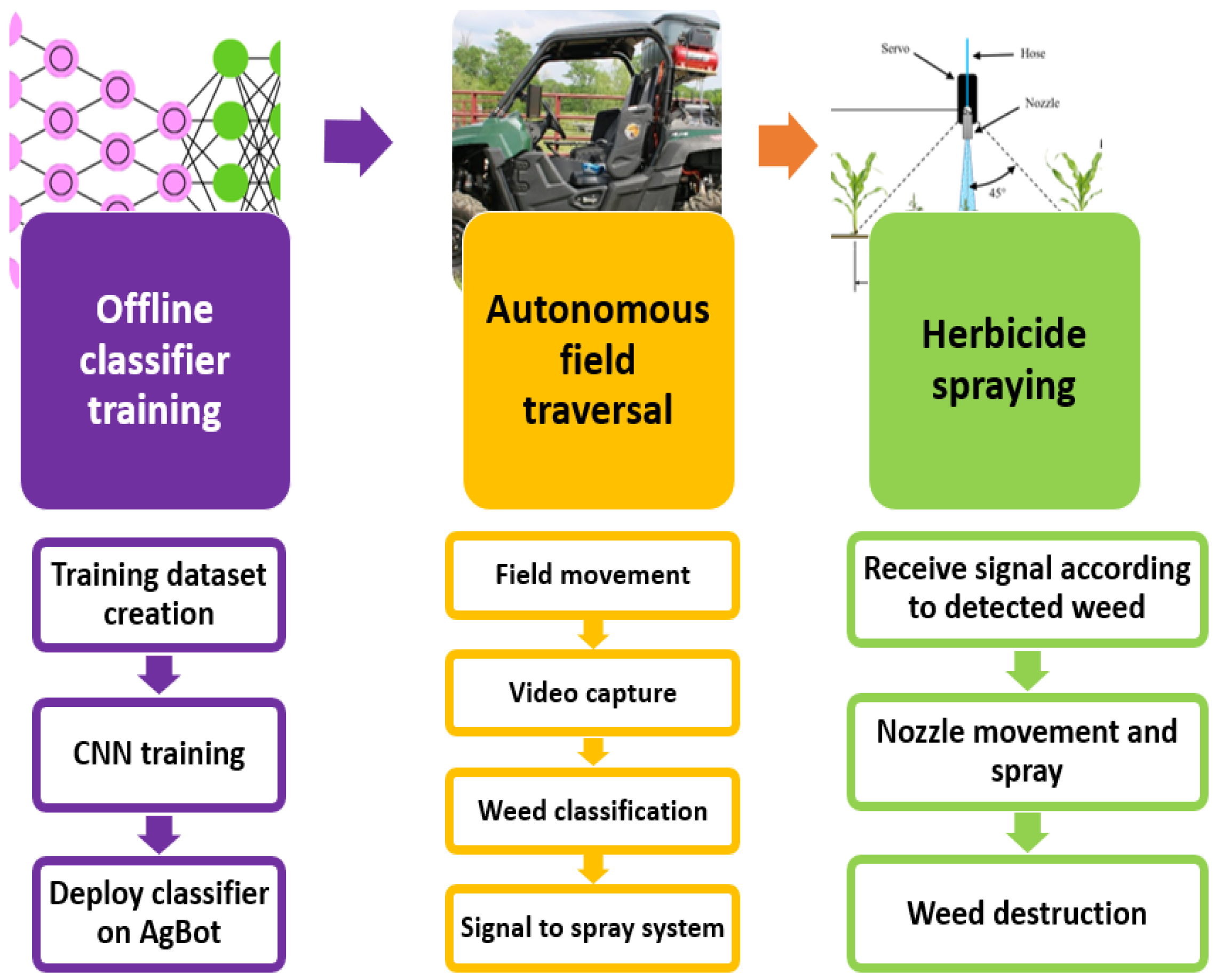
• Real-Time Deployment on Autonomous Agricultural Platform (AgBOT): The retrained model was deployed on AgBOT with a monocular RGB camera. The performance was evaluated under real operating conditions, including varying illumination, occlusion, and motion-induced noise. The system demonstrates $F_1$ scores of 0.96, 0.94, and 0.95 for Cocklebur, Pigweed, and Ragweed, respectively. The overall classification accuracy is observed to be 94%. Moreover, the model achieves an average inference time of 0.266 s on CPU and 0.032 s on GPU, confirming the suitability of the approach for real-time applications.
• Design and Evaluation of Multi-Sensor Fusion Algorithm: While the single-sensor setup shows promising results, its performance degrades under specific scenarios such as partial occlusion or sensor malfunction, leading to misclassification and unreliable control signals for downstream actuators (e.g., herbicide sprayers). To mitigate this, the study introduces a decision-level fusion strategy incorporating time domain and space domain reasoning.

Time domain fusion smooths classification outputs over a fusion time window $t_s$. The algorithm detects inconsistency in predictions from a given sensor over time and penalizes unstable outputs. Experimental evaluation shows that setting $t_s=10$ s effectively stabilizes classifications in the presence of a faulty sensor (Figure 14), while $t_s=3$ s is sufficient to handle temporary occlusions (Figure 16). This temporal smoothing significantly improves the robustness of the CNN output in dynamic field environments. Space domain fusion utilizes redundancy across multiple sensors to isolate and correct faulty outputs. When one sensor provides data that significantly deviates from the consensus among the sensor array, its influence is down-weighted. The algorithm dynamically adapts to sensor disagreements, thereby preventing misclassification due to isolated failures. This approach is particularly effective in detecting outliers caused by sensor dropouts or environmental interference. The combined fusion framework ensures that even if one or more sensors exhibit inconsistent or erroneous behavior, the overall classification system remains stable and accurate. In test scenarios, the system consistently mitigated classification anomalies arising from challenging conditions such as partial occlusion or sensor drift.

Overall, this study demonstrates that combining transfer learning with a robust sensor fusion framework can significantly improve weed classification accuracy and reliability under real-world conditions. The architecture is computationally efficient, scalable, and suitable for real-time deployment on autonomous agricultural robots. By addressing both temporal and spatial uncertainties in sensor outputs, the proposed system provides a fail-safe mechanism for mission-critical agricultural operations like targeted herbicide spraying.

5. Conclusions

This study presents a multi-sensor fusion algorithm for improved weed classification using real-time camera image data for autonomous precision weeding with transfer learning-based CNN, assuming prior weed species knowledge. For a small image dataset, transfer learning avoids the complex and labor-intensive step of hard-coded feature extraction from images and provides higher accuracy compared to a CNN model built from scratch. We re-trained a VGG16 with a small weed dataset and demonstrated that the model shows sufficient test accuracy and moderate inference time, adequate for real-time applications. Implementation of the weed detection model in real-time applications via an Autonomous AgBot using a single camera was observed to run into classification instability in challenging scenarios such as noise, vibration, and occlusion. To overcome the limitations of the single-camera feed, we proposed a multi-camera sensor fusion algorithm by utilizing a Dempster–Shafer combination rule. The test result shows that not only the final weed classification output from the multi-sensor system with sensor-fusion algorithm is robust and accurate in scenarios like noise and vibration, which eliminates the classification instability, but also it can handle challenging operating conditions such as faulty sensors or partial occlusion very well and provide reliable output to be used for applications in herbicide spraying.

It is important to emphasize that there are some limitations to this method, which we plan to address in future studies. Since time domain fusion is highly sensitive to the choice of time window ($t_s$), selecting a longer $t_s$ may excessively smooth the output and reduce system responsiveness, while a shorter $t_s$ might not effectively suppress transient noise. Similarly, space domain fusion depends on the number of integrated sensors; while a higher number of sensors increases redundancy and improves decision reliability, it also adds to the system’s complexity and cost. Therefore, a trade-off exists between temporal responsiveness, spatial robustness, and overall system efficiency. Careful tuning of $t_s$ and sensor array size is necessary to achieve an optimal balance between classification accuracy, inference latency, and resource consumption.

In this study, we primarily focused on detecting a single weed within the camera frame. In future work, this research can be extended to handle multiple weeds in a single frame and to evaluate system performance across different crop fields and various weed species. These extensions will help assess the scalability and robustness of the proposed system in more diverse and realistic agricultural environments.

References

1. Gilbert, N. Case studies: A hard look at GM crops. Nat. News 2013, 497, 24–26. [Google Scholar] [CrossRef]
2. Khan, N.; Medlock, G.; Graves, S.; Anwar, S. GPS Guided Autonomous Navigation of a Small Agricultural Robot with Automated Fertilizing System; Technical Report, SAE Technical Paper; SAE International: Warrendale, PA, USA, 2018. [Google Scholar]
3. Fung, M.L.; Chen, M.Z.; Chen, Y.H. Sensor fusion: A review of methods and applications. In Proceedings of the 2017 29th Chinese Control And Decision Conference (CCDC), Chongqing, China, 28–30 May 2017; pp. 3853–3860. [Google Scholar]
4. Heinrich, S.; Motors, L. Flash memory in the emerging age of autonomy. In Proceedings of the Flash Memory Summit, Santa Clara, CA, USA, 8–10 August 2017; pp. 1–10. [Google Scholar]
5. Singh, V.; Singh, D. Development of an Approach for Early Weed Detection with UAV Imagery. In Proceedings of the IGARSS 2022—2022 IEEE International Geoscience and Remote Sensing Symposium, Kuala Lumpur, Malaysia, 17–22 July 2022; pp. 4879–4882. [Google Scholar] [CrossRef]
6. Reedha, R.; Dericquebourg, E.; Canals, R.; Hafiane, A. Transformer Neural Network for Weed and Crop Classification of High Resolution UAV Images. Remote Sens. 2022, 14, 592. [Google Scholar] [CrossRef]
7. Moazzam, S.I.; Khan, U.S.; Nawaz, T.; Qureshi, W.S. Crop and Weeds Classification in Aerial Imagery of Sesame Crop Fields Using a Patch-Based Deep Learning Model-Ensembling Method. In Proceedings of the 2022 2nd International Conference on Digital Futures and Transformative Technologies (ICoDT2), Rawalpindi, Pakistan, 24–26 May 2022; pp. 1–7. [Google Scholar] [CrossRef]
8. Ahmad, M.; Adnan, A.; Chehri, A. A Real-Time IoT and Image Processing based Weeds Classification System for Selective Herbicide. In Proceedings of the 2022 IEEE 95th Vehicular Technology Conference: (VTC2022-Spring), Helsinki, Finland, 19–22 June 2022; pp. 1–5. [Google Scholar] [CrossRef]
9. Ota, K.; Louhi Kasahara, J.Y.; Yamashita, A.; Asama, H. Weed and Crop Detection by Combining Crop Row Detection and K-means Clustering in Weed Infested Agricultural Fields. In Proceedings of the 2022 IEEE/SICE International Symposium on System Integration (SII), Narvik, Norway, 9–12 January 2022; pp. 985–990. [Google Scholar] [CrossRef]
10. Chen, Y.; Wu, Z.; Zhao, B.; Fan, C.; Shi, S. Weed and corn seedling detection in field based on multi feature fusion and support vector machine. Sensors 2020, 21, 212. [Google Scholar] [CrossRef]
11. Rodríguez-Garlito, E.C.; Paz-Gallardo, A.; Plaza, A. Automatic Detection of Aquatic Weeds: A Case Study in the Guadiana River, Spain. IEEE J. Sel. Top. Appl. Earth Obs. Remote Sens. 2022, 15, 8567–8585. [Google Scholar] [CrossRef]
12. Garibaldi-Márquez, F.; Flores, G.; Mercado-Ravell, D.A.; Ramírez-Pedraza, A.; Valentín-Coronado, L.M. Weed Classification from Natural Corn Field-Multi-Plant Images Based on Shallow and Deep Learning. Sensors 2022, 22, 3021. [Google Scholar] [CrossRef]
13. Potena, C.; Nardi, D.; Pretto, A. Fast and accurate crop and weed identification with summarized train sets for precision agriculture. In Proceedings of the International Conference on Intelligent Autonomous Systems, Shanghai, China, 3–7 July 2016; pp. 105–121. [Google Scholar]
14. Sharpe, S.M.; Schumann, A.W.; Yu, J.; Boyd, N.S. Vegetation detection and discrimination within vegetable plasticulture row-middles using a convolutional neural network. Precis. Agric. 2020, 21, 264–277. [Google Scholar] [CrossRef]
15. Reddy, L.U.K.; Rohitharun, S.; Sujana, S. Weed Detection Using AlexNet Architecture In The Farming Fields. In Proceedings of the 2022 3rd International Conference for Emerging Technology (INCET), Belgaum, India, 27–29 May 2022; pp. 1–6. [Google Scholar] [CrossRef]
16. Espejo-Garcia, B.; Mylonas, N.; Athanasakos, L.; Fountas, S.; Vasilakoglou, I. Towards weeds identification assistance through transfer learning. Comput. Electron. Agric. 2020, 171, 105306. [Google Scholar] [CrossRef]
17. Sunil, G.; Zhang, Y.; Koparan, C.; Ahmed, M.R.; Howatt, K.; Sun, X. Weed and crop species classification using computer vision and deep learning technologies in greenhouse conditions. J. Agric. Food Res. 2022, 9, 100325. [Google Scholar] [CrossRef]
18. Yu, J.; Sharpe, S.M.; Schumann, A.W.; Boyd, N.S. Deep learning for image-based weed detection in turfgrass. Eur. J. Agron. 2019, 104, 78–84. [Google Scholar] [CrossRef]
19. Al-Badri, A.H.; Ismail, N.A.; Al-Dulaimi, K.; Rehman, A.; Abunadi, I.; Bahaj, S.A. Hybrid CNN Model for Classification of Rumex Obtusifolius in Grassland. IEEE Access 2022, 10, 90940–90957. [Google Scholar] [CrossRef]
20. Olsen, A.; Konovalov, D.A.; Philippa, B.; Ridd, P.; Wood, J.C.; Johns, J.; Banks, W.; Girgenti, B.; Kenny, O.; Whinney, J.; et al. DeepWeeds: A multiclass weed species image dataset for deep learning. Sci. Rep. 2019, 9, 2058. [Google Scholar] [CrossRef] [PubMed]
21. Du, Y.; Zhang, G.; Tsang, D.; Jawed, M.K. Deep-CNN based Robotic Multi-Class Under-Canopy Weed Control in Precision Farming. In Proceedings of the 2022 International Conference on Robotics and Automation (ICRA), Philadelphia, PA, USA, 23–27 May 2022; pp. 2273–2279. [Google Scholar] [CrossRef]
22. Dodge, S.; Karam, L. Understanding how image quality affects deep neural networks. In Proceedings of the 2016 Eighth International Conference on Quality of Multimedia Experience (QoMEX), Lisbon, Portugal, 6–8 June 2016; pp. 1–6. [Google Scholar]
23. Wang, A.; Zhang, W.; Wei, X. A review on weed detection using ground-based machine vision and image processing techniques. Comput. Electron. Agric. 2019, 158, 226–240. [Google Scholar] [CrossRef]
24. Rodrigo, M.; Oturan, N.; Oturan, M.A. Electrochemically assisted remediation of pesticides in soils and water: A review. Chem. Rev. 2014, 114, 8720–8745. [Google Scholar] [CrossRef] [PubMed]
25. Marshall, E. Field-scale estimates of grass weed populations in arable land. Weed Res. 1988, 28, 191–198. [Google Scholar] [CrossRef]
26. Tian, L.; Reid, J.F.; Hummel, J.W. Development of a precision sprayer for site-specific weed management. Trans. ASAE 1999, 42, 893–900. [Google Scholar] [CrossRef]
27. Medlin, C.R.; Shaw, D.R. Economic comparison of broadcast and site-specific herbicide applications in nontransgenic and glyphosate-tolerant Glycine max. Weed Sci. 2000, 48, 653–661. [Google Scholar] [CrossRef]
28. Åstrand, B.; Baerveldt, A.J. An agricultural mobile robot with vision-based perception for mechanical weed control. Auton. Robot. 2002, 13, 21–35. [Google Scholar] [CrossRef]
29. Choi, Y.K.; Lee, S.J. Development of advanced sonar sensor model using data reliability and map evaluation method for grid map building. J. Mech. Sci. Technol. 2015, 29, 485–491. [Google Scholar] [CrossRef]
30. Shalal, N.; Low, T.; McCarthy, C.; Hancock, N. A preliminary evaluation of vision and laser sensing for tree trunk detection and orchard mapping. In Proceedings of the Australasian Conference on Robotics and Automation (ACRA 2013), Sydney, Australia, 2–4 December 2013; pp. 1–10. [Google Scholar]
31. Garcia-Alegre, M.C.; Martin, D.; Guinea, D.M.; Guinea, D. Real-time fusion of visual images and laser data images for safe navigation in outdoor environments. In Sensor Fusion-Foundation and Applications; IntechOpen: London, UK, 2011. [Google Scholar]
32. Farooq, A.; Jia, X.; Hu, J.; Zhou, J. Transferable Convolutional Neural Network for Weed Mapping With Multisensor Imagery. IEEE Trans. Geosci. Remote Sens. 2022, 60, 4404816. [Google Scholar] [CrossRef]
33. Gai, J.; Tang, L.; Steward, B. Plant localization and discrimination using 2D+ 3D computer vision for robotic intra-row weed control. In Proceedings of the 2016 ASABE Annual International Meeting, Orlando, FL, USA, 17–20 July 2016; p. 1. [Google Scholar]
34. Rosebrock, A. Deep Learning for Computer Vision with Python: Starter Bundle; PyImageSearch: Philadelphia, PA, USA, 2017. [Google Scholar]
35. Chollet, F. Deep Learning mit Python und Keras: Das Praxis-Handbuch vom Entwickler der Keras-Bibliothek; MITP-Verlags GmbH & Co. KG: Frechen, Germany, 2018. [Google Scholar]
36. Simonyan, K.; Zisserman, A. Very deep convolutional networks for large-scale image recognition. arXiv 2014, arXiv:1409.1556. [Google Scholar]
37. Mohanty, S.P.; Hughes, D.P.; Salathé, M. Using deep learning for image-based plant disease detection. Front. Plant Sci. 2016, 7, 1419. [Google Scholar] [CrossRef] [PubMed]
38. Karpathy, A.; Toderici, G.; Shetty, S.; Leung, T.; Sukthankar, R.; Fei-Fei, L. Large-scale video classification with convolutional neural networks. In Proceedings of the IEEE Conference on Computer Vision and Pattern Recognition, Columbus, OH, USA, 23–28 June 2014; pp. 1725–1732. [Google Scholar]
39. Ramcharan, A.; Baranowski, K.; McCloskey, P.; Ahmed, B.; Legg, J.; Hughes, D. Using Transfer Learning for Image-Based Cassava Disease Detection. arXiv 2017, arXiv:1707.03717. [Google Scholar]
40. Khan, M.N.; Anwar, S. Paradox Elimination in Dempster–Shafer Combination Rule with Novel Entropy Function: Application in Decision-Level Multi-Sensor Fusion. Sensors 2019, 19, 4810. [Google Scholar] [CrossRef] [PubMed]
41. Jiang, W.; Luo, Y.; Qin, X.Y.; Zhan, J. An improved method to rank generalized fuzzy numbers with different left heights and right heights. J. Intell. Fuzzy Syst. 2015, 28, 2343–2355. [Google Scholar] [CrossRef]
42. Dempster, A.P. Upper and lower probabilities induced by a multivalued mapping. In Classic Works of the Dempster-Shafer Theory of Belief Functions; Springer: Berlin/Heidelberg, Germany, 2008; pp. 57–72. [Google Scholar]
43. Shafer, G. A Mathematical Theory of Evidence; Princeton University Press: Princeton, NJ, USA, 1976; Volume 42. [Google Scholar]
44. Bossé, E.; Roy, J. Fusion of identity declarations from dissimilar sources using the Dempster-Shafer theory. Opt. Eng. 1997, 36, 648–657. [Google Scholar] [CrossRef]
45. Dasarathy, B.V. Sensor Fusion: Architectures, Algorithms, and Applications VI. In Proceedings of the Sensor Fusion: Architectures, Algorithms, and Applications VI, Orlando, FL, USA, 3–5 April 2002; Volume 4731. [Google Scholar]
46. Jiang, W.; Wei, B.; Liu, X.; Li, X.; Zheng, H. Intuitionistic fuzzy power aggregation operator based on entropy and its application in decision making. Int. J. Intell. Syst. 2018, 33, 49–67. [Google Scholar] [CrossRef]
47. Ma, J.; Liu, W.; Miller, P.; Zhou, H. An evidential fusion approach for gender profiling. Inf. Sci. 2016, 333, 10–20. [Google Scholar] [CrossRef]
48. Zhang, L.; Ding, L.; Wu, X.; Skibniewski, M.J. An improved Dempster–Shafer approach to construction safety risk perception. Knowl.-Based Syst. 2017, 132, 30–46. [Google Scholar] [CrossRef]
49. Yuan, K.; Xiao, F.; Fei, L.; Kang, B.; Deng, Y. Modeling sensor reliability in fault diagnosis based on evidence theory. Sensors 2016, 16, 113. [Google Scholar] [CrossRef]
50. Sabahi, F. A novel generalized belief structure comprising unprecisiated uncertainty applied to aphasia diagnosis. J. Biomed. Inform. 2016, 62, 66–77. [Google Scholar] [CrossRef]
51. Deng, Y. Deng Entropy: A Generalized Shannon Entropy to Measure Uncertainty. 2015. Available online: http://vixra.org/pdf/1502.0222v1.pdf (accessed on 16 July 2025).
52. Ye, F.; Chen, J.; Tian, Y. A robust DS combination method based on evidence correction and conflict redistribution. J. Sens. 2018, 2018, 6526018. [Google Scholar] [CrossRef]
53. Khan, M.N.; Anwar, S. Time-Domain Data Fusion Using Weighted Evidence and Dempster–Shafer Combination Rule: Application in Object Classification. Sensors 2019, 19, 5187. [Google Scholar] [CrossRef] [PubMed]
54. Tammina, S. Transfer learning using vgg-16 with deep convolutional neural network for classifying images. Int. J. Sci. Res. Publ. 2019, 9, 143–150. [Google Scholar] [CrossRef]
55. Bali, S.; Tyagi, S. Evaluation of transfer learning techniques for classifying small surgical dataset. In Proceedings of the 2020 10th International Conference on Cloud Computing, Data Science & Engineering (Confluence), Noida, India, 29–31 January 2020; pp. 744–750. [Google Scholar]
56. Kaur, T.; Gandhi, T.K. Automated brain image classification based on VGG-16 and transfer learning. In Proceedings of the 2019 International Conference on Information Technology (ICIT), Bhubaneswar, India, 19–21 December 2019; pp. 94–98. [Google Scholar]
57. Murphy, R.R. Dempster-Shafer theory for sensor fusion in autonomous mobile robots. IEEE Trans. Robot. Autom. 2002, 14, 197–206. [Google Scholar] [CrossRef]
58. Yong, D.; WenKang, S.; ZhenFu, Z.; Qi, L. Combining belief functions based on distance of evidence. Decis. Support Syst. 2004, 38, 489–493. [Google Scholar] [CrossRef]
59. Han, D.Q.; Deng, Y.; Han, C.Z.; Hou, Z.Q. Weighted evidence combination based on distance of evidence and uncertainty measure. J. Infrared Millim. Waves 2011, 30, 396–400. [Google Scholar] [CrossRef]
60. Wang, J.; Xiao, F.; Deng, X.; Fei, L.; Deng, Y. Weighted evidence combination based on distance of evidence and entropy function. Int. J. Distrib. Sens. Netw. 2016, 12, 3218784. [Google Scholar] [CrossRef]
61. Jiang, W.; Wei, B.; Xie, C.; Zhou, D. An evidential sensor fusion method in fault diagnosis. Adv. Mech. Eng. 2016, 8, 1687814016641820. [Google Scholar] [CrossRef]
Figure 1. Retrofitted Yamaha Wolverine side-by-side with ATV AgBot.
Computation 13 00174 g001
Figure 2. A simplified representation of the transfer learning process.
Computation 13 00174 g002
Figure 3. The proposed decision-level sensor fusion architecture in this research.
Computation 13 00174 g003
Figure 4. Simplified representations of time domain and space domain fusion processes.
Computation 13 00174 g004
Figure 5. Classification and spray system pipeline of the AgBot.
Computation 13 00174 g005
Figure 6. Sample images of the weed dataset.
Computation 13 00174 g006
Figure 7. Training and validation accuracy.
Computation 13 00174 g007
Figure 8. Six-layer CNN architecture.
Computation 13 00174 g008
Figure 13. Sensor fault detection via time and space domain fusion.
Computation 13 00174 g013
Figure 14. Ground truth value for Ragweed and Pigweed shown at the top. (a) Classification accuracy from left, center, and right cameras for Pigweed. (b) Classification accuracy from the left, center, and right cameras for Rigweed. (c) Stable classification output (smooth curve) with time domain fusion. (d) Eliminated the effect of faulty sensor (right camera) evidence on final classification output with space domain fusion.
Computation 13 00174 g014
Figure 15. Improved classification for partially occluded weed data with space domain sensor fusion.
Computation 13 00174 g015
Figure 16. Ground truth value for Ragweed and Pigweed at the top. (a) Classification accuracy from left, center, and right cameras for Pigweed. (b) Classification accuracy from left, center, and right cameras for Rigweed. (c) Reduced classification error (smooth curve) with time domain fusion. (d) Eliminated the effect of partial occlusion on final classification output with space domain fusion.
Computation 13 00174 g016